Automatic Identification of Experts and Performance Prediction in the Multimodal Math Data Corpus through Analysis of Speech Interaction

Automatic Identification of Experts and Performance

Prediction in the Multimodal Math Data Corpus through

Analysis of Speech Interaction

Saturnino Luz

School of Computer Science and Statistics Department of Computer Science

Trinity College Dublin Dublin, Ireland

[email protected]

ABSTRACT

An analysis of multiparty interaction in the problem solv-ing sessions of the Multimodal Math Data Corpus is pre-sented. The analysis focuses on non-verbal cues extracted from the audio tracks. Algorithms for expert identification and performance prediction (correctness of solution) are im-plemented based on patterns of speech activity among ses-sion participants. Both of these categorisation algorithms employ an underlying graph-based representation of dia-logues for each individual problem solving activities. The proposed Bayesian approach to expert prediction proved quite effective, reaching accuracy levels of over 92% with as few as 6 dialogues of training data. Performance predic-tion was not quite as effective. Although the simple graph-matching strategy employed for predicting incorrect solu-tions improved considerably over a Monte Carlo simulated baseline (F1 score increased by a factor of 2.3), there is still

much room for improvement in this task.

Categories and Subject Descriptors

H.3.1 [Information Storage and Retrieval]: Content Analysis and Indexing; I.5.2 [Pattern Recognition]: Clas-sifier design and evaluation

Keywords

Collaborative problem solving, Multimodal Math Data Cor-pus, vocalisation graphs

1.

INTRODUCTION

Beyond speech transcription and analysis of high-level con-tent, it has become increasingly clear that paralinguistic and multimodal features hold important clues as to the nature of group interaction in a number of contexts [5, 17, 19, 4,

Permission to make digital or hard copies of all or part of this work for personal or classroom use is granted without fee provided that copies are not made or distributed for profit or commercial advantage and that copies bear this notice and the full cita-tion on the first page. Copyrights for components of this work owned by others than ACM must be honored. Abstracting with credit is permitted. To copy otherwise, or re-publish, to post on servers or to redistribute to lists, requires prior specific permission and/or a fee. Request permissions from [email protected].

ICMI’13,December 9–13, 2013, Sydney, Australia Copyright 2013 ACM 978-1-4503-2129-7/13/12 ...$15.00. http://dx.doi.org/10.1145/2522848.2533788.

12]. In learning and problem solving situations involving groups, in particular, there is evidence that low-level speech features such as speech duration, energy and prosody, and writing features such as writing rate, area, aspect ratio, and pressure are predictors of social dominance and expertise [20].

This paper describes approaches to the 2013 Multimodal Learning Analytics (MMLA) challenges which are based on simple non-verbal speech interaction features (namely, struc-ture and amount of talk, including simultaneous talk, and silence). In brief, these challenges consist in, 1) identifying the domain expert among groups of three students working cooperatively on mathematical problem solving tasks and 2) inferring, from group interaction during a problem solv-ing task, whether the group answered the question correctly or incorrectly. We conceptualise these challenges as cat-egorisation tasks and refer to them simply as the “expert identification task” and the “performance prediction task”, respectively. The data set employed in this MMLA chal-lenge, the Multimodal Math Data Corpus, is described in detail in [16]. A benchmark analysis is presented in [15].

A few differences between the approach reported in this paper and other uses of low-level speech features in predic-tion tasks, such as in speech act classificapredic-tion [21] and detec-tion of decision points [6], among others, should be pointed out. First, we restrict ourselves to the above mentioned low-level speech features. No other information source, in-cluding video, writing, past performance (as in the bench-mark study [15], for instance) is employed. This does not imply that we believe such features to be of lesser value for this task. Quite on the contrary. We simply wish to assess the particular contribution those speech features can make. Second, we make no use of prosodic features (speech rate, pitch, loudness) other than pause duration, though we dis-cuss briefly how these features could be incorporated into our data representation scheme in future work (section 6). Third, we structure speech features as a vocalisation graph [5, 13] rather than consider them in isolation.

those works so as to abstract away speaker information. This is done so that we can deal with the performance prediction task in a completely general (i.e. session and speaker inde-pendent) way, on a nearest-neighbour framework. For the expert detection task, we derive general interaction statis-tics from each vocalisation graph (representing a problem-solving dialogue) and employ a strategy based on voting among naive Bayes classifiers. These approaches yielded mixed results. The speaker prediction task was quite suc-cessful within sessions. The correction prediction task was less effective. This is partly due to the imbalanced nature of the data (only 19% of answers fall into the “incorrect” category, and these are unevenly distributed across the vari-ous sessions and groups, making negative prediction harder), and partly due to the somewhat crude graph matching algo-rithm we employed to determine nearest neighbours. How-ever, we believe that these problems are not insurmountable and that this graph based approach to performance predic-tion also shows some promise.

2.

DATA PREPARATION

The original MLA corpus comprises data collected from 6 distinct, gender-matched groups of 3 students each, work-ing on algebra and geometry problems over 12 sessions (2 separate sessions per group). Each session consisted of 16 problem solving tasks, in which the students worked coop-eratively and mentored one another. The students were be-tween 15 to 17 years old, and were grouped according to their skill levels.

The corpus made available to the participants of the ICMI MLA challenge includes, for each session: 4 audio streams (3 streams containing individual speaker audio, recorded through close-talking microphones, and 1 stream containing all audio, recorded through an omnidirectional microphone placed above the participants), 4 video streams (recorded through 3 individual cameras and 1 wide-angle camera, avail-able in both high and low resolution versions), 3 digital pen log files (1 per student), and annotated metadata. The an-notation includes, for each of task: time boundaries (start and end of problem solving, start and end of “moment of in-sight”, time to solution), performance data (time to solution and correctness), participation data (student who initiated the answer, and the student who explained the answer, when prompted), and coding of the digital pen data.

At the session level, the metadata provided with the cor-pus includes the identities (participant codes) of the group leaders and dominant experts for each session. A partici-pant’s expertise is defined in terms of a cumulative score of points assigned to correctly and incorrectly solved problems, weighted according a discrete difficulty level scale (“easy”, “moderate” , “hard”). The session expert is the student with the highest such expertise score. A detailed description of the tasks, the participant profiles, the data collection pro-cedure and the data set can be found in the accompanying documentation [16].

The MLA corpus provides a rich resource for the analy-sis of different aspects of interaction in educational settings. However, for the purposes of the work reported in this paper, only the individual (close-talking) audio streams, the task-level timing information, and the correctness and expertise coding (to identify the target categories for classification) have been used. The processing of these data and the re-sulting new data sets are described next.

2.1

Generating vocalisation graph data sets

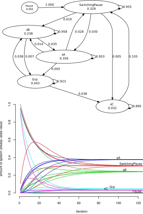
Initially, the audio files were processed in order to detect speech intervals (vocalisations) and to assign these intervals unique speaker identifiers (or the identifier “Group vocalisa-tion” for intervals containing overlapping speech by two or more speakers). Since the individual recordings were fairly free from noise, we could employ a simple voice activity de-tection algorithm to generate time stamps for vocalisation intervals. For each speaker’s audio file, the signal was re-sampled at 100ms intervals, and for each sample we marked it as a potential vocalisation (and stored it) if it exceeded an energy threshold of -36dB, otherwise it was marked as silence. Consecutive silence intervals exceeding 1s in dura-tion indicated the end of a vocalisadura-tion, at which point the time stamps of stored vocalisation samples were smoothed and stored as an array. The arrays containing individual vocalisation profiles were then merged into a single stream of vocalisation events. From these vocalisation streams, we generated transition matrices encoding Markov chains such as the one shown in Figure 1 (top).

iteration

amount of speech (steady−state v

alue)

0 20 40 60 80 100 120

0.0

0.2

0.4

0.6

0.8

1.0

Pause SwitchingPause

sB sA

Grp sC

Figure 1: An individuated vocalisation graph repre-senting the dialogue of group 1, solving problem 1A in session 1 (top) and its convergence to a steady state (bottom).

to imply that we considerallsuch non-verbal events irrele-vant. In fact, there is evidence (from other domains) that non-verbal speech sounds such as laughter and “fillers” have clear roles in structuring the dialogue [4, 2]. On the other hand, those very short bursts of audio activity would have had a detrimental effect on categorisation had they not been removed. This effect has also been observed in topic segmen-tation tasks [11].

A vocalisation event can be: a vocalisation, containing speech a participant’s speech turn, apause, or an interval greater than 1s in which all participants have fallen silent (we further distinguish “switching pauses”, or silence interval between vocalisations by different speakers [5]), or agroup vocalisation, where two or more speakers speak at the same time. See [12] for a more formal definition. Each entry in the vocalisation matrix represents the probabilityP(Vj|Vi)

that a vocalisation eventViwill be followed by a vocalisation

eventVj, where typical transitions include, for instance, a

speakersstarting to speak after a pause, a speakers initiat-ing a turn and beinitiat-ing interrupted by speakert, an interval of silence followed by two speakers speaking at the same time, and so on.

A vocalisation graph is a Markov chain containing a sin-gle aperiodic recurrent class, which means that the tran-sition probabilities always converge to steady state proba-bilities by iterating the Chapman-Kolmogorov equation, as the number of iterations increases. Figure 1 (bottom) shows this convergence for the corresponding vocalisation graph (shown at the top). We define two kinds of vocalisation graphs: “individuated graphs” (like the one shown in Fig-ure 1) and “aggregated graphs”. Aggregated vocalisation graphs do not distinguish between speakers but rather pool all vocalisations into a single node.

For performance prediction (i.e. prediction of correct vs incorrect solution) we employed aggregated vocalisations graphs, since our aim has been to make this task entirely indepen-dent of sessions and groups. That is, we aim to find fea-tures that generalise across all problem solving dialogue in-stances. For expert identification, on the other hand, we created a feature set based on individuated graphs (omit-ting, of course, the specific speaker identification tags).

2.2

Expert identification data set

Expert identification posed a problem for the above-described graph representation schema. Recall that we have formu-lated the problem as a categorisation task. That is, given a data instance representing a speaker our goal is to label that data instance with an expert or an non-expert category tag. Therefore we cannot identify individual nodes explic-itly in the representation. Neither, for the same reason, can we identify speaker to speaker transitions.

In face of this difficulty, we chose to represent each speaker

s in each problem solving dialogue d as an octuple of the form:

s= [vΣ, vµ, vσ, p(s|f), p(f|s), p(s|g), p(g|s), H(V|s)] (1)

where:

vΣ is the total duration of all vocalisations produced by

speakers,

vµ is the average duration of the vocalisations produced by

speakers,

vσ is the standard deviation of vocalisations produced by

speakers,

p(s|f) is the probability of a transition from “floor” (i.e. a pause, group switching pause or speaker switching pause) to a vocalisation produced by speakers,

p(f|s) is the probability of a transition from a vocalisation by speakers to floor (i.e. that speakers falls silent and no other speaker speaks for at least 1 second),

p(s|g) is the probability of transitioning from a group vo-calisation to a speakersvocalisation,

p(g|s) is the probability of transitioning from a speakers

vocalisation to a group vocalisation,

H(V|s) is the Shannon entropy of a vocalisation event V

conditioned on a speakersvocalisation event, that is, a measure of uncertainty in the transitions (turn taking) originating from speakers, given by

H(V|s) =−X

v

P(v|s)log2P(v|s)

This representation is independent of speaker identity, group session and problem task dialogue and was generated uniformly for the entire MLA data set.

As regards our choice of features, it seems plausible that the level of expertise of a speaker (as related to their con-tributions to solving problems correctly) correlates with the amount of speech they produce and the regularity with which they produce their spoken contributions. Features vΣ, vµ

andvσ are meant to capture this putative regularity. It also

seems reasonable to expect that the dominant speaker would tend to initiate turns, after moments of silence, and perhaps take most turns following a moment of simultaneous speech. Features p(s|f) and p(s|g) quantify such situations. Simi-larly, featuresp(f|s) andp(g|s) reflect the extent to which a speaker’s vocalisation yields silence (perhaps indicating writing activity) and simultaneous verbal activity (perhaps indicating disagreement), respectively. Finally, the entropy feature the uniformity with which vocalisation events are distributed in succession to a speaker’s vocalisation. Ex-perts are expected to exhibit more predictable vocalisation sequence patterns (i.e. they are expected to be more consis-tent in their contributions). In fact, preliminary data anal-ysis reveals a weak (ρ=−0.18) but reliable (p <0.01) cor-relation between amount of speech and entropy, indicating that more verbally active speakers are also more predictable in terms of the turn taking patterns they originate.

2.3

Performance prediction data set

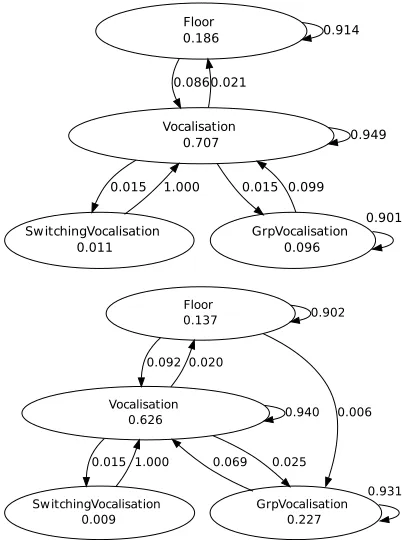
lot more overlapping speech (group vocalisations), less si-lence and less turn taking. Our working hypothesis is that these kinds of difference reflect dialogue regularities that have predictive value in this task.

Figure 2: Aggregated vocalisation graphs showing dialogues resulting in correct (top) and incorrect (bottom) answers, for problems of similar difficulty levels.

As is the case of the representation set out in equation (1), this graph representation can be generated uniformly for the entire corpus (it can, in fact, be generated for any di-alogue). However, for categorisation purposes, the matrix representation for these vocalisation graphs has been “flat-tened” into 40-tuple instances, each feature representing one of the 4 + 6×6 possible vocalisations and transitions, as explained in section 4.

3.

EXPERT IDENTIFICATION

A continuous-variable naive Bayes approach was employed for expert prediction. For each speakersa, . . . sc in a

prob-lem solving task dialogue, described by features V1, . . . V8

as in equation (1), the probability that this speaker will be labelled an expert is given by equation (2), which can be rewritten as (3) under the usual conditional independence assumption.

P(t|s) ∝ P(V1=sΣ, . . . , V8=H(V|s)|t) (2)

=

n

Y

i=1

P(Vi=vi|t) (3)

The estimation procedure for the conditionals in (3) mod-els the vocalisation features through Gaussian kernmod-els, as shown in equation (4), whereµt andσt2 are the mean and

variance of the values taken by the features Vi in the data

set given a positive expert label, represented here as Boolean

t. Non-parametric estimation methods also exist [9] but we have not tried them in this task.

P(Vi=x|b) = g(x;µt, σt)

= 1

σt

√

2πe

−(x−µt)2

2σ2_{t (4)}

These models were trained on a portion of a session’s data and subsequently used to estimate probabilities for each speaker instance in the testing problem solving dialogues. Expert inference consisted in taking a vote among the esti-mates, so that and expert labels∗was assigned to the most likely instance:

s∗= arg max

s∈{sa...,sc}

P(t|s) (5)

Similarly, one could apply a voting strategy to identify an expert for the overall session rather than individual in-stances by choosing the mode of the set of labels produced by evaluating all individual instances in the test set.

3.1

Expert identification results

There are different ways of going about identifying domain experts in a corpus of recorded problem solving dialogues, and at least two distinct ways of framing the problem.

As regards expert identification methods, one could base the system’s inference on domain knowledge, or try to in-ductively learn such knowledge from relatively unstructured data. Oviatt [15], for instance, presents a rule-base method that selects as expert the participant who answers the most of the firstn problems correctly (alternatively, the partici-pant that initiates the most of the firstnanswers). The ap-proach we adopted here, on the other hand, requires training data in the form of instances that describe the participants’ speech interactions during a problem solving session in or-der to learn which instance most closely resembles the speech activity of the expert.

With respect to framing the prediction problem itself, there are, so to speak, a more general and a more specific way of looking at it. A more general perspective would de-fine the task of the system as follows: given a single dialogue (say, a set of participant interaction instances) recorded dur-ing a problem solvdur-ing activity, identify the participant who is characterised as the domain expert in the session (containing several such dialogues) during which the dialogue in question took place. This is the harder version of the problem. The specific, and somewhat easier version of the problem can be formulated as follows: given a problem solving session (as a set of dialogue representations), identify the participant characterised as the expert. The above described rule-based approach would achieve 50% accuracy [15, p. 7] in the most general formulation, since it would have to base its decision on the features of a single problem. However, in the easier formulation, the rule-based approach performs quite well, being able to correctly guess the expert after seeing only 7 problem instances.

Table 1: Expert prediction accuracy for different numbers of training dialogues averaged over predic-tions for dialogues and grouped by sessions.

# training mean accuracy dialogues by dialogue(sd) by session

1 0.54 (0.22) 0.67 2 0.58 (0.27) 0.75 3 0.55 (0.29) 0.67 4 0.60 (0.18) 0.83 5 0.61 (0.18) 0.75 6 0.62 (0.17) 0.92 7 0.70 (0.14) 1.00

training instances; one per speaker) and averaged the accu-racy results over the 12 sessions. The results are shown in Table 1.

The mean accuracy by dialogue corresponds to the more general formulation. The average reported is across all ses-sions, and the number of training dialogues refers to the training data for each individual session. On the sixth row, for instance, the 62% accuracy score was obtained by train-ing the system on 6 dialogues (18 speaker instances described as in equation (1)) per session, testing on the remaining 9 di-alogues and averaging the results over all sessions (standard deviation of 0.17). As the training set increases in size so do the accuracy and the stability of predictions, as indicated by decreasing standard deviations.

The figures for accuracy per session correspond to the more specific formulation. As in [15] we report the accu-racy scores obtained as the system “sees” progressively more dialogues of a session (though in our case the position of the problem in the session is irrelevant). For this setting we trained the models in the same way as before, but identi-fied the expert as the one who matched the chosen expert speaker label in most dialogues of a session (or rather, most dialogues in the test set of a session). In this case, if the system is presented with, say, 6 dialogues (training set) and infers the expert for the session by choosing the majority label assigned to the remaining 10 dialogues it infers the session expert correctly for 92% of the sessions. Likewise, 7 training dialogues suffice to identify all experts correctly in all sessions. The relatively low accuracy figures in the sec-ond column (mean accuracy by dialogue) compared to the third (mean accuracy per session) reflect the fact that the former assesses classification of individual dialogues, where the system makes no use of the knowledge that a particular speaker is identified as the expert foralldialogues in a par-ticular session. It is tempting therefore to speculate that in some problem solving sessions certain speakers exhibit ex-pert behaviour even though they may not do so throughout the session.

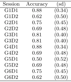
We also ran 4-fold cross validation tests per session in or-der to get a better idea of expert prediction performance by dialogue (general formulation) in each session. The mean accuracy results are shown in Table 2. In most (though not all) cases, prediction performance degrades in sessions that have different speakers as assigned session leader and expert. It seems therefore that the expert leader role adds a measure of “noise” to those data folds by altering the relative amount of talk produced by non-expert leaders. However, perfor-mance in all cases is well above the 33% baseline, indicating

Table 2: Mean expert prediction accuracy scores for 4-fold cross-validation experiments per session.

Session Accuracy (sd) G1D1 0.88 (0.34) G1D2 0.62 (0.50) G2D1 0.75 (0.45) G2D2 0.69 (0.48) G3D1 0.81 (0.40) G3D2 0.81 (0.40) G4D1 0.88 (0.34) G4D2 0.69 (0.48) G5D1 0.50 (0.52) G5D2 0.69 (0.48) G6D1 0.75 (0.45) G6D2 0.62 (0.50)

that the method is quite robust, even in the presence of this sort of noise.

4.

PERFORMANCE PREDICTION

As mentioned before, the MLA corpus is quite imbalanced with respect to the questions answered correctly and incor-rectly. The overall distribution is 81% for correct answers versus 19% incorrect answers. Class imbalance is known to cause difficulties to most machine learning methods [8]. To complicate matters, the balance of positive and negative in-stances varies greatly from session to session, reflecting the different levels of expertise of the 6 groups. Thus, the pro-portion of correct answers varies from 38% in G2D1 to 100% in G2D2 and G5D2.

In order to minimise this problem, we have used the en-tire data set for evaluation, ignoring group and session sub-divisions. This also means that we attempted to model cor-rectness and incorcor-rectness prediction in the most general setting, in which classification does not depend on features that are specific to a group of participants. To this end, ag-gregated vocalisation graphs of the kind shown in Figure 2 were employed in this task.

The classification method is based on ak nearest neigh-bour strategy [1]. The “training” of the system consists sim-ply in storing the training instances. Classification was per-formed by finding the vocalisation graph (or graphs) most similar to the test instance and assigning it the category of that training instance (or the majority label, in case there are more than one such neighbours). Instance similarity was defined in terms of the Euclidean distance

d(s, t) = v u u t

n

X

i=1

(Vt i −Vis)2

between instances, taking into account the n= 40 features representing all transition probabilities in the graph.

4.1

Performance prediction results

Table 3: Precision, recall and F1 results for the

performance prediction task. Values denote means computed over a 10-fold cross validation.

System hypotheses Correct Incorrect Precision: 0.850 Precision: 0.375 Recall: 0.826 Recall: 0.417

F1: 0.838 F1: 0.395

Baselines (Monte Carlo) Correct Incorrect Precision: 0.805 Precision: 0.178 Recall: 0.809 Recall: 0.193

F1: 0.802 F1: 0.193

“classifier” that labelled all instances “correct”) would have accuracy of 80% on average. We therefore provide a finer grained evaluation broken down into metrics for each class (“correct” and “incorrect”) separately. These metrics include precision (ratio of the number of true positives to the total number of items categorised as the target category by the system), recall (ratio of the number of true positives to the total number of items in the target category) andF1 (the

harmonic mean of precision and recall).

Table 3 summarises the results. As expected, the “incor-rect” category proved to be much harder to predict than the “correct” category. With respect to the former, the system performs quite poorly. It detects just over 41% of problems that are solved incorrectly. Furthermore, of the problems it flags as incorrect solutions, nearly two thirds are false alarms.

However, to put these results into perspective, we propose comparing them to a Monte Carlo baseline. The baseline scores shown in Table 3 were obtained by simulating 190 classification 100 times and averaging the precision, recall and F1 results. The categorisation decisions in these

sim-ulations can be regarded as “informed guesses”, since they were the result of sampling the two possible categories ac-cording to category generalities proportional to the general-ities observed in the actual data set. In comparison to this baseline, the system categorisation results for the “incorrect” class represent a marked improvement, while no performance degradation is observed for the “correct” class.

It should also be remarked that the group 5 sessions are atypical in that they are extremely imbalanced. In fact, one of them (G5D2) does not contain a single error. If these sec-tions are removed, a slight improvement in prediction per-formance can be observed.

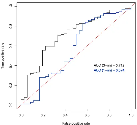
In all cases, however, the models produced had fairly weak diagnostic power in general. A useful summary of overall predictive power is given by the area under the ROC (re-ceiver operating characteristic) curve [3]. The ROC curve is a plot of the true positive rate (or recall) against the false positive rate (specificity) as the classification threshold is varied. Figure 3 shows the ROC the curves for a nearest neighbour model and a 3 nearest neighbour model, where the probabilities for the classification thresholds were ob-tained by weighting the neighbours proportionally to the inverse of their distance to the query instance. The diag-onal represents chance classification. It can be seen from the ROC chart that the voting strategy employed by the

3-Figure 3: Area under the ROC curve for nearest neighbour (lower curve, in blue) and 3-NN (higher curve, in black) models evaluated over the 12 ses-sions of the MLA corpus.

NN model improves the overall quality of the classifier, even though the improvement in terms of F-score for the negative class (incorrect answers) is negligible.

5.

DISCUSSION

The accuracy results obtained by the graph vocalisation method for expert identification presented in this paper are comparable to the benchmark results reported by Oviatt [15]. In fact, our results show certain advantages of our approach with respect to that benchmark. The method pre-sented there works by keeping a count of the number of times a participant initiated an answer or correctly solved a prob-lem. However, since the number of correct solutions forms part of the definition of expertise according to the annota-tion schema, and since the accuracy of soluannota-tions is directly proportional to the overall number of solutions initiated (i.e. participants who contribute many solutions are more likely to contribute correct answers than incorrect ones), classi-fication based on these features appears to be of limited informative value.

The method described here, in contrast, only employs low-level speech features that can be easily extracted from speech recorded through close-talking microphones and require no content analysis as such. Yet, despite their simplicity, these features seem to generalise well over different groups and levels of skill. With this feature set based on vocalisation graphs, a naive Bayes classifier required very few instances to attain a reasonable level of accuracy.

chal-lenges in performance prediction is the uneven and imbal-anced distribution of correct and incorrect solutions in the MLA corpus. Since detecting incorrect solution would in-tuitively appear to be more important from an applications perspective than simply acknowledging correct solutions, a cost sensitive classification approach may be required for this task.

The models we have tested so far essentially employ a zero-one loss function, so that classification decisions penalise all miscategorisations equally (i.e. λ(T, F) =λ(F, T) = 1 and

λ(T, T) = λ(F, F) = 0, whereλ is a loss function). Given that the data set is imbalanced, such a function will tend to improve accuracy for the overall session at the expense of the dialogues that resulted in incorrect answers. A cost sensitive approach would choose a threshold (defined, as illustrated in Figure 3, in terms of probabilities) so as to penalise miscat-egorisations of negative instances (incorrect answers) more than positive ones.

6.

CONCLUSION AND FURTHER WORK

This paper reported on our initial experiments with vo-calisation based (“content free”) approaches to expertise de-tection and performance prediction in problem solving ac-tivities by small groups of students.

Overall, the results look promising. The expertise detec-tion task was performed quite accurately based on a simple, 8-feature summary of vocalisation transitions, in problem solving dialogues, from the point of view of each speaker. The performance prediction results were poorer, but never-theless improved upon a simulated baseline, suggesting that the graph based approach can play a role in a performance prediction method that includes other data sources. Re-stricted to the speech modality alone, one possible avenue for improvement would be to devise a more effective graph similarity measure to mitigate the effect of the relatively high dimensionality which seems to impair the method em-ployed so far. We expect that this, in combination with a cost sensitive classification approach as outlined above would improve the prediction performance in this challenging task. We also plan on incorporating richer features into the vocalisation graph framework. Speech features could be refined, for instance, by incorporating detection of laugh-ter, fillers, hesitation markers and other non-verbal speech sounds [4]. In addition, features from the video and writing streams could also be incorporated into the data representa-tion. It has been suggested that even fairly low-level features extracted from recorded written interaction in combination with vocalisation data can be effective in helping browsers of meeting recordings structure and visualise [10] intervals and actions of potential interest in the data [14]. Further work on multimodal learning analytics could build on this research.

7.

ACKNOWLEDGEMENTS

This study was part-funded by the Science Foundation Ireland through the Centre for Next Generation Localisa-tion (CNGL), grant number 07/CE/1142. The author also wishes to thank the anonymous reviewers of this ICMI MMLA Grand Challenge for their insightful comments and sugges-tions.

8.

REFERENCES

[1] D. Aha and D. Kibler. Instance-based learning algorithms.Machine Learning, 6:37–66, 1991. [2] F. Bonin, N. Campbell, and C. Vogel. Laughter and

topic changes: Temporal distribution and information flow. In P. Baranyi, editor,3rd IEEE Conference on Cognitive Infocommunications, pages 53–58, 2012. [3] A. P. Bradley. The use of the area under the ROC

curve in the evaluation of machine learning algorithms.

Pattern Recognition, 30(7):1145–1159, July 1997. [4] N. Campbell. On the use of nonverbal speech sounds

in human communication. In A. Esposito, M. Faundez-Zanuy, E. Keller, and M. Marinaro, editors,Verbal and nonverbal communication

behaviours, Lecture Notes in Computer Science, pages 117–128. Springer, 2007.

[5] J. M. J. Dabbs and B. Ruback. Dimensions of group process: Amount and structure of vocal interaction.

Advances in Experimental Social Psychology, 20(123–169), 1987.

[6] P.-Y. Hsueh and J. D. Moore. Automatic decision detection in meeting speech. In A. Popescu-Belis, S. Renals, and H. Bourlard, editors,Machine Learning for Multimodal Interaction (MLMI ’07), volume 4892 ofLecture Notes in Computer Science. Springer, 2007. [7] J. Jaffe and S. Feldstein.Rhythms of dialogue.

Academic Press, New York, 1970.

[8] N. Japkowicz and S. Stephen. The class imbalance problem: A systematic study.Intelligent Data Analysis, 6(5):429–449, 2002.

[9] G. H. John and P. Langley. Estimating continuous distributions in Bayesian classifiers. In Besnard, Philippe and S. Hanks, editors,Proceedings of the 11th Conference on Uncertainty in Artificial Intelligence (UAI’95), pages 338–345, San Francisco, CA, USA, Aug. 1995. Morgan Kaufmann Publishers.

[10] S. Luz. Interleave factor and multimedia information visualisation. In H. Sharp, P. Chalk, J. LePeuple, and J. Rosbottom, editors,Proceedings of Human

Computer Interaction 2002, volume 2, pages 142–146, London, 2002.

[11] S. Luz. Locating case discussion segments in recorded medical team meetings. InProceedings of the ACM Multimedia Workshop on Searching Spontaneous Conversational Speech (SSCS’09), pages 21–30, Beijing, China, Oct. 2009. ACM Press.

[12] S. Luz. The non-verbal structure of patient case discussions in multidisciplinary medical team

meetings.ACM Transactions on Information Systems, 30(3):article 17, 2012.

[13] S. Luz and B. Kane. Classification of patient case discussions through analysis of vocalisation graphs. In

Proceedings of the 11th International Conference on Multimodal Interfaces and Machine Learning for

Multimodal Interaction (ICMI-MLMI’09), pages

107–114, Cambridge, MA, 2009. ACM.

[15] S. Oviatt. Problem-solving, domain expertise and learning: Ground-truth performance results for math data corpus. InSecond International Workshop on Multimodal Learning Analytics, Sydney, Australia, dec 2013.

[16] S. Oviatt, A. Cohen, and N. Weibel. Multimodal learning analytics: Description of math data corpus for ICMI grand challenge workshop. Available fromhttp: //mla.ucsd.edu/data/MMLA_Math_Data_Corpus.pdf, 2013. Accessed August 2013.

[17] A. Pentland. Social signal processing [exploratory DSP].IEEE Signal Processing Magazine,

24(4):108–111, 2007.

[18] R Development Core Team.R: A Language and Environment for Statistical Computing. R Foundation for Statistical Computing, Vienna, Austria, 2011. ISBN 3-900051-07-0.

[19] S. Renals, T. Hain, and H. Bourlard. Recognition and interpretation of meetings: The AMI and AMIDA projects. InProc. IEEE Workshop on Automatic

Speech Recognition and Understanding (ASRU ’07),

2007.

[20] S. Scherer, N. Weibel, L.-P. Morency, and S. Oviatt. Multimodal prediction of expertise and leadership in learning groups. InProceedings of the 1st

International Workshop on Multimodal Learning Analytics, MLA ’12, pages 1:1–1:8. ACM, 2012. [21] E. Shriberg, A. Stolcke, D. Jurafsky, N. Coccaro,

M. Meteer, R. Bates, P. Taylor, K. Ries, R. Martin, and C. van Ess-Dykema. Can prosody aid the

automatic classification of dialog acts in conversational speech? Language and Speech, 41(3-4):443–492, 1998.

APPENDIX

A.

SOURCE CODE AND DERIVED DATA

SETS

The source code for the algorithms presented in this paper, and the new data and annotations produced in the course of this work are available for download from our GitLab server. The the most recent version of the source code and derived data sets that are necessary to replicate the results described above can be obtained bygit clone’ing the fol-lowing repository:

http://gitlab.scss.tcd.ie/saturnino.luz/icmi-mla-challenge.git

The current (“frozen”) version of the code and data is also available from the author’s website at

https://www.scss.tcd.ie/~luzs/software/icmi-mla2013.tgz

Please note that the MMLA corpus itself is subject to a non-disclosure agreement and is therefore not distributed with the packages above. The data distributed in these pack-ages consist solely of the derived vocalisation graphs needed to perform the categorisation experiments.