Abstract –In this paper, the methods of structural and
parametric synthesis of a RoboMech class parallel manipulator with two end-effectors are presented. This parallel manipulator is formed by connecting the two moving output objects with the fixed base by two passive, one active and two negative closing kinematic chains. Geometrical parameters of the active and negative closing kinematic chains are determined by the Chebyshev and least-square approximations.
Index Terms - Parallel manipulator, end-effector, structural-parametric synthesis.
I. INTRODUCTION
Depending on the type of technological operation, the robot manipulator can operate in two modes: a simultaneous manipulation of two objects and a sequential manipulation of one object.
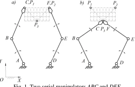
[image:1.595.51.286.434.585.2]In the simultaneous manipulation of two objects, two serial manipulators ABC and DEF handle two objects in the initial positions P1 and P2 (Fig. 1a), then two objects are moved to the specified position P3 (Fig. 1b). Next, the manipulators return to their initial positions.
Fig. 1. Two serial manipulators ABC and DEF.
In the sequential manipulation of one object, the first serial manipulator ABC handles the object in the position P1 (Fig. 1a), then the object is moved to the intermediate position P3, where the object is transferred to the gripper of the second serial manipulator DEF (Fig. 1b). Next, the object is moved by the second serial manipulator DEF to the specified position P2 (Fig. 1b).
Manuscript received March 2019.
Zh. Baigunchekov, Zh. Zhumasheva, B. Naurushev, A. Mustafa, R. Kairov, B. Amanov are with the Research and Educational Centre “Digital Technologies and Robotics”, Al-Farabi Kazakh National University and Department of Applied Mechanics, Satbayev University, Almaty, Kazakhstan (e-mail: [email protected]).
For example, a printing machine operates in the mode of sequential manipulation of one object. In this machine, a blank sheet of paper is fed by the first manipulator onto the printing table, and the second manipulator picks up the sheet after printing. This cyclical process occurs in a short period of time. Therefore, in such automatic machines, instead of two serial manipulators, it is advisable to use one manipulator (mechanism) with two end-effectors and one DOF. The parallel manipulators (PM) of a class RoboMech belong to such manipulators. PM having the property of manipulation robots such as a reproducing the specified laws of motions of the end-effectors, and the property of mechanisms such as a setting the laws of motions the actuators which simplify the control system and increase speed, are called PM of a class RoboMech [1-3].
In this paper, the methods of structural-parametric synthesis of a RoboMech class PM with two end-effectors are developed. There are many methods of structural and kinematic (parametric or dimensional) synthesis of mechanisms [4-6], where the kinematic synthesis of mechanisms is carried out for their given structural schemes. In this case, it is possible that a given structural scheme of the mechanism may not provide the specified laws of motions of the end-effectors. Therefore, it is necessary to carry out the kinematic synthesis together with the structural synthesis. The methods of structural-parametric synthesis allow to simultaneously determine the optimal structural schemes of PM and the geometrical parameters of their links according to the given laws of motions of the end-effectors and actuators.
II. STRUCTURAL SYNTHESIS
According to the developed principle of forming mechanisms and manipulators [1,2], the PM with two end-effectors is formed by connecting two output objects with a fixed base using closing kinematic chains (CKC), which can be active, passive and negative. If we connect these two output objects with the fixed base by two passive CKC ABC
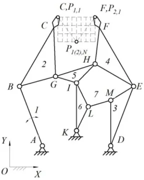
and DEF, having zero DOF, we obtain two serial manipulators (Fig. 2). In the paper [7], a PM of the fifth class with two end-effectors and two DOF (Fig. 2) was formed from these two serial manipulators by connecting the links 2 and 4 by the negative CKC GH of type RR, then by connecting the link GH with a fixed base by the negative CKC IK type RR, and by connecting the links IK and DE by the negative CKC LM of type RR, where R is a revolute kinematic pair. Each of the binary links of type RR has one negative DOF. The disadvantages of this PM is a small workspace because the links 2 and 4 of two serial manipulators ABC and DEF are connected by one link GH.
Parallel Manipulator of a Class RoboMech with
Two End-Effectors
Fig. 3. PM with two end-effectors of the fifth class. The workspace of the PM with two end-effectors can be increased by connecting the links 2 and 4 of the serial manipulators ABC and DEF by the active CKC GHKI with active kinematic pair K. As a result, we obtain PM
ABGHKIED with three DOF, where the links AB, KH and
DE are input links (Fig. 3). For formation of a RoboMech class PM with one DOF, we connect the links 1 and 5, as well as the links 3 and 6 by the negative CKC ML and NQ
of type RR. As a result, we obtain a structural scheme of a RoboMech class PM with two end-effectors, which has the following structural formula
[image:2.595.89.250.474.678.2]IV(1,2,5,8)I(0,8)IV(3,4,6,9). (5) Therefore, the formed RoboMech class PM consists of an input link 7 and two fourth class Assur groups, or two Stephenson II mechanisms with the common input link 7.
Fig. 2. PM of a class RoboMech with two end-effectors. Thus, this RoboMech class PM with two end-effectors is formed by connecting of two output objects with a fixed base by two passive CKC ABC and DEF, one active CKC
GHKI and two negatives CKC LM and NQ.
Since the active and negative CKC impose geometrical constraints on the motions of the output objects, then the
formed PM of a RoboMech class with two end-effectors works at certain values of the geometrical parameters (synthesis parameters) of the links. Passive CKC doesn’t impose geometrical constraints on the motions of output objects, therefore, their synthesis parameters vary taking into account the superimposed geometrical constraints of the connecting active and negative CKC. Consequently, the problem of parametric synthesis of the whole RoboMech class PM with two end-effectors is reduced to the subproblems of parametric synthesis of its structural modules (passive, active and negative CKC). Such a modular representation of structural - parametric synthesis simplifies the problem of designing of PM. Let consider the parametric synthesis of the structural modules of the RoboMech class PM with two end-effectors.
III. PARAMETRIC SYNTHESIS OF STRUCTURAL MODULES
Given N discrete values of the grippers centers C and F
coordinates , and , ( 1, 2,..., )
i i i i
C C F F
X Y X X i N .
The synthesis parameters of two passive CKC ABC and
DEF (or serial manipulators) are
, and
, , , , , ,
A A AB BC D D DE EF
X Y l l X Y l l whereX YA, A and XD,YD
are coordinates of the pivot joints A and D in the absolute coordinate system OXY; lAB,lBC DE,l ,lEFare lengths of the links AB,BC,DE,EF. The synthesis parameters of the passive CKC vary using the «LP sequence» [8].
The synthesis parameters of the active CKC GHKI are
(2) (2) (4) (4) (7) (7)
, y , I , yI , H , yH , K, K, GH, HI, G G
x x x X Y l l where
(2) (2) (4) (4) (7) (7)
, y , I ,yI , H , yH G G
x x x are coordinates of the joints
G, I, H in the moving coordinate systems
2 2, 4 4, 7 7,
Bx y Ex y Kx y fixed to the links BC, EF, KH, respectively; XK,YK are coordinates of the pivot joint K in the absolute coordinate system OXY; lGH, lIH are lengths of the links GH, IH.
Write the vector loop-closure equations of OKHGBO and
OKHIEO
(7) (2)
7 ( ) 2
( ) ( )
i i
K i H HG B i G
R Γ r l R Γ r , (2)
(7) (4)
7 ( ) 4
( ) i i ( ) ,
K i H HI E i I
R Γ r l R Γ r (3)
where RK
XK,YK
T, rH(7) xH(7),yH(7)T,( )i cos ( )i, sin ( )i ,
T HG lHG
HG lHG
HG l
,
T ,Bi XBi YBi
R
(2) (2), (2) T, (7) (7), (7) T,
H H H
G xG yG x y
r r
( ) ( ) ( )
(4) (4) (4)
cos , sin ,
, , , ,
i i i
i i i
T
HI HI HI HI HI
T T
E E E I I I
l l
X Y x y
l
R r
( )
cos( ) sin( )
( ) .
sin( ) cos( )
Γ
The angles
2i and
4i in the Eqs (2) and (3), which determine the positions of the links ВС and EF of the passive CKC АВС and DEF, are calculated from the analysis of positions of these CKC by the expressions1
2 tg i i
i i
C B
i
C B
Y Y
,
X X
(4)
1
4 tg i i
i i
F E
i
F E
Y Y
,
X X
(5) where
1 1 cos
, sin
Bi A i
AB
Bi A i
Х X
l
Y Y
(6)
3 3 cos
. sin
Ei D i
DE
Ei D i
Х X
l
Y Y
(7)
The angles
1i and
3i in Eqs (6) and (7) are determined by the expressions2 2 2
1 1
1 tg cos 2
2
i i
i i
C A AC AB BC
i
C A AC AB
Y Y l l l
,
X X l l
(8)
2 2 2
1 1
3 tg cos 2
2
i i
i i
F D DF DE EF
i
F D DF DE
Y Y l l l
,
X X l l
(9)
where
2
2 21i i i
AC C A C A
l X X Y Y ,
2
2 21i i i
DF F D F D
l X X Y Y .
Eliminating the unknown angles
( HG )i and
( HI )i, from Eqs (2) and (3) yields2
(7) (2) 2
7 2
( ) ( ) 0,
i
K i H B i G lHG
R Γ r R Γ r (10)
2
(7) (4) 2
7 4
( ) ( ) 0,
i
K i H E i I lHI
R Γ r R Γ r (11)
Eqs (10) and (11) are the equations of geometrical constraints imposed on the motion of two output objects. The geometric meaning of Eqs (10) and (11) are the equations of two circles with radiuses lHG and lHI in relative motions of the planes Bx y2 2 and Bx y4 4relative to
the planeKx y7 7. The problem of determining the geometrical parameters of the links at which such geometrical constraints are approximately realized is the problem of parametric synthesis of the active CKC GHKI.
The left parts of Eqs (10) and (11) are denoted by
(1) 1i q
and q2(2)i , which are functions of weighted differences
2
(1) (7) (2) 2
7 2
1i K ( i)H Bi ( i)G HG,
q l
R Γ r R Γ r (12)
2
(2) (7) (4) 2
7 4
2i K ( i)H Ei ( i) I HI 0.
q l
R Γ r R Γ r (13)
After converting these equations and the following change of variables
2 2 2 2
(2) (7)
6 4
1
(2) (7)
5
2 7
(7) (7) (2) (2)
2 2 2
3
, , ,
y y
1
( y y ),
2
G
K H
K G H
K K H H G G HG
x p x p
p X
p
p Y p
p X Y x x l
2 2 2 2
(4) 8
(4) 9
(7) (7) (4) (4)
2 2 2
10
, y 1
( y y )
2
I
I
K K H H I I HI
x p p
p X Y x x l
the functions q1iand q2i are represented as linear forms by groups p1( )j and p2( )k of synthesis parameters
( ) ( ) ( ) ( )
1 2 1 1 01 , ( 1, 2,3), T
j j j j
i i i
q g j
g p (14)
( ) ( ) ( ) ( )
2 2 2 2 02 , ( 1, 2,3), T
k k k k
i i i
q g k
g p (15)
where
4 6
2 7
(1)
5 7
1
0 0
( ) ( )
0 0 ,
0 0 1 0 0 0 1 0
1 i
i B
i i
B i
X p p
Y p p
Γ Γ
g
1 6
2 7 2
(2)
2 7
2
0 0
( ) ( )
0 0 ,
0 0 1 1 0 0 1 0
i
i B T
i i i
B i
X p p
Y p p
Γ Γ
g
1 4
7 7 2
(3)
2 5
3
0 0
( ) ( )
0 0 ,
0 0 1 1 0 0 1 0
i
i B T
i i i
B i
p X p
p Y p
Γ Γ
2
7 7 2
4
(1) 2 2
01 5 6 6 4 5 7 7 1 [ , ] ( ) 2 [ , ] ( ) , ( ) ,
i i i
i i
i i i i i
B B
i B B
B B
p g X Y X Y
p
p p
X Y p p
p p Γ Γ Γ
76
(2) 2 2
1 2
01
7
1
[ , ] ( ) ,
2 i i Bi Bi i
i B B
p
g X Y p X p Y
p Γ
74
(3) 2 2
1 2
01
5
1
[ , ] ( ) ,
2 i i Bi Bi i
i B B
p
g X Y X p Y p
p Γ 8 6 4 7 (1) 9 7 2 0 0 ( ) ( )
0 0 ,
0 0 1 0 0 0 1 0
1 i i E i i E i
X p p
Y p p
Γ Γ g 1 6
4 7 4
(2)
2 7
2
0 0
( ) ( )
0 0 ,
0 0 1 1 0 0 1 0
i
i E T
i i i
E i
X p p
Y p p
Γ Γ g 1 8
7 7 4
(3)
2 9
3
0 0
( ) ( )
0 0 ,
0 0 1 1 0 0 1 0
i
i E T
i i i
E i
p X p
p Y p
Γ Γ g
47 7 4
8
(1) 2 2
02 9 6 6 8 9 7 7 1 [ , ] ( ) 2 [ , ] ( ) , ( ) ,
i i i
i i
i i i i i
E E
i E E
E E
p g X Y X Y
p
p p
X Y p p
p p Γ Γ Γ
76
(2) 2 2
1 2
02
7
1
[ , ] ( ) ,
2 i i Ei Ei i
i E E
p
g X Y p X p Y
p
Γ
78
(3) 2 2
1 2
02
9
1
[ , ] ( ) .
2 i i Ei Ei i
i E E
p
g X Y X p Y p
p Γ
The linear representability of the geometrical constraints Eqs (14) and (15) with respect to the groups p1( )j and p( )2k of synthesis parameters allows to formulate the following approximation problems of parametric synthesis:
-Chebyshev approximation, - least-square approximation
to determine the groups p1( )j and p( )2k of synthesis parameters.
In the Chebyshev approximation problem, the vectors of synthesis parameters are determined from the minimum of the functionals
1
1
1 1 1 1 1
1,
( ) max (j)( ) min ( ),
(j) i
(j) (j) (j) (j) (j) i N
S q S
p
p p p
(16)
2
2
2 2 2 2 2
1,
( ) max (k)( ) min ( ).
(k) i
(k) (k) (k) (k) (k) i N
S q S
p
p p p
(17)
In the least-square approximation problem, the vectors of synthesis parameters are determined from the minimum of the functionals
1 1
1 1 1 1
1
( ) (j) min ( ),
(j) i
N
(j) (j) (j) (j) i
S q S
p p p (18) 2 22 2 2 2
1
( ) (k) min ( ),
(k) i
N
(k) (k) (k) (k) i
S q S
p p p (19)Since the synthesis parameters of the active CKC GHKI
are simultaneously included in functionals (16-19), their values are determined by joint consideration of the functionals (16) and (17), and also (18) and (19).
The linear representability of Eqs (12) and (13) in the forms (14) and (15) allows for solving the Chebyshev approximation problem (16) and (17), to apply the kinematic inversion method, which is an iterative process, at each step of which one group of synthesis of the parameters
( ) 1
j
p and p( )2k is defined. In this case, the problem of linear programming is solved by four parameters. To do this, we introduce a new variable p11, where is a required accuracy of the approximation. Then the minimax problems (16) and (17) are reduced to the following linear programming problem: determine the minimum of the sum
min , T
х c x (20)where
0,..., 0,1
, ( ), 11 TT j k
c x р p with the following
restrictions ( ) ( ( )) ( ( )) 1(2) 01(2) 11 ( ) ( ( )) ( ( )) 1(2) 01(2) 11 1 , 2 1 , 2 j k
j k j k
i i
j k
j k j k
i i p p р g g р g g (21)
The sequence of the obtained values of the functions
( ( )) ( ( ))
1(2) ( )
j k j k
S p will decrease and have a limit as a sequence bounded below, because S1(2)( ( ))j k (p( ( ))j k )0 for anyp( ( ))j k . Let consider the solution of the least-square approximation problem (18) and (19) for the synthesis of the considered active CKC GHKI. From the necessary conditions for the minimum of functions S1(2)( ( ))j k by groups
( ( )) 1(2)
j k
p of synthesis parameters
( ( )) 1(2) ( ( )) 1(2) 0 j k j k S
we obtain the systems of linear equations in the forms
( ( )) ( ( )) ( ( ))
1(2) 1(2) 1(2) , ( , 1, 2, 3).
j k j k j k j k
H p h (23)
Solving the systems of equations (23) for each group of synthesis parameters for given values of the remaining parameter groups, we determine their values
( ( )) ( ( )) 1 ( ( ))
1(2) 1(2) 1(2)
j k j k j k
p H h
(24).
It is not difficult to show that the Hessian H1(2)( ( ))j k is positively defined together with the main minors. Then the solutions of the systems (23) correspond to the minimum of the functions S1(2)( ( ))j k . Consequently, the least-square approximation problem for parametric synthesis is reduced to the linear iteration method, at each step of which the systems of linear equations are solved.
Let consider the solution of parametric synthesis problem of the negative CKC LM and NQ. For this, we preliminarily determine the positions of the synthesized active CKClinks of the GH and IH
2 2 2
1 1
5 tg -cos
2
i i i
i i
i
GH IH GI
I G i
I G lGI GH
l l l
Y Y
,
X X l
(25)
1
6 tg i i
i i
H I
i
H I
Y Y
,
X X
(26) where
(2)
2 2
(2)
2 2
cos sin
, o
sin c s
i i
i i
G B i i G
i i G B
G
Х X x
Y Y y
(4)
4 4
(4)
4 4
cos sin
, sin cos
i i
i i
I E i i I
i i I E
I
Х X x
Y Y y
1
2 2 2
i i i i
I I G I G
G
l X X Y Y ,
5
5 cos
. sin
i i
i i
H G i
GH i H G
Х X
l
Y Y
Write the vector loop-closure equations of OBGMLAO
and OEINQDO
(5) (1)
5 1
( ) ( ) ,
i
i i M ML A i L
G
R Γ r l R Γ r (27)
(6) (3)
6 3
( ) ( ) ,
i i
I i N NQ D i Q
R Γ r l R Γ r (28)
where , , (5) (5), (5) ,
i i i
T T
G XG YG M xM yM
R r
i cos i, sin i ,
,
,T
T
ML ML ML ML A A A
ML l l X Y
l R
(1) (1) (1) (6) (6) (6)
( )
(3) (3) (3)
, , , , , ,
cos , sin ,
, , , .
i i i
i i i
T T T
I I I
L L L N N N
T
NQ NQ NQ NQ NQ
T T
D D D Q Q Q
x y X Y x y
l l
X Y x y
r R r
l
R r
Eliminating the unknown angles
i
ML
and
i
NQ
from
Eqs (27) and (28) yields
2
(5) (1) 2
5 1
( ) ( ) 0,
i i M A i I ML
G l
R Γ r R Γ r (29)
2
(6) (3) 2
6 3
( ) ( ) 0.
i NQ
I i N D i Q l
R Γ r R Γ r (30)
Eqs (29) and (30) are the equations of geometrical constraints imposed on the motions of links 1 and 5, 3 and 6 by the negative CKC ML and NQ. The geometrical meanings of these constraints are the equations of two circles in the relative motions of the planes of links 1 and 5, 3 and 6 with radiuses lML and lNQ. The problem of determining the geometrical parameters of the links, at which such geometric constraints are approximately realized, is the problem of parametric synthesis of two negative CKC ML and NQ.
The left parts of Eqs (29) and (30) are denoted by
3i q
and q4i, which are functions of weighted differences
2
(5) (1) 2
3i Gi ( 5i) M A ( 1i)1i ML,
q l
R Γ r R Γ r (31)
2
(6) (3) 2
4i Ii ( 6i) H D ( 3i)Q NQ.
q l
R Γ r R Γ r (32)
After converting these equations and the following change of variables
2 2 2 2
(1) (5)
14 11
(1) (5)
15 12
(1) (1) (5) (5) 2
13
, ,
y y
1
( y y ),
2
L M
L M
LM
L L M M
x p x
p
p p
p x x l
2 2 2 2
(3) (5)
16 19
(3) (5)
17 20
(3) (3) (6) (6) 2
18
, ,
y y
1
( y y )
2
Q N
N Q
QN
N N
Q Q
x x
p p
p p
p x x l
(1) (2)
11 12 13 14 15 13
3 [ , , ] , 3 [ , , ] ,
T T
p p p p p p
p p
(1) (2)
16 17 18 19 20 18
4 [ , , ] , 4 [ , , ]
T T
p p p p p p
p p
in the forms
( ) ( ) ( ) ( )
3 2 3 3 03 , ( 1, 2),
j j j j
i i i
q g j
g p (33)
( ) ( ) ( ) ( )
4 2 4 4 04 ,( 1, 2),
T
k k k k
i i i
q g k
g p (34) where
1 14
1 2 1
(1)
15 3
0 0
( ) ( )
0 0 ,
0 0 1 1 0 0 1 0
i
i G A
i i i
G A i
X X p
Y Y p
Γ Γ
g
1 1 11
2 2 1
(2)
12 3
0 0
( ) ( )
0 0 ,
0 0 1 1 0 0 1 0
i
i G A
i i i
G A i
X X p
Y Y p
Γ Γ
g
2
2 2
(1) 03
14
15
1
2
, ( ) ,
i i
i
i i
A A
i G G
A A
G G
g X X Y Y
p
X X Y Y
p
Γ
1
2 2
(2) 03
11
12
1
2
, ( ) ,
i i
i
i i
A A
i G G
A A
G G
g X X Y Y
p
X X Y Y
p
Γ
1 19
3 4 3
(1)
20
4 ,
0 0
( ) ( )
0 0
0 0 1 1 0 0 1 0
i i
I D
i i i
I D i
X X p
Y Y p
Γ Γ
g
1 1 16
4 4 3
(2)
17 4
0 0
( ) ( )
0 0 ,
0 0 1 1 0 0 1 0
i
i I D
i i i
I D i
X X p
Y Y p
Γ Γ
g
4
2 2
(1) 04
19
20
1
2
, ( ) ,
i i
i
i i
D D
i I I
D D
I I
g X X Y Y
p
X X Y Y
p
Γ
3
2 2
(2) 04
16
17
1
2
, ( ) .
i i
i
i i
D D
i I I
D D
I I
g X X Y Y
p
X X Y Y
p
Γ
Further, on the basis of the approximation problems of the Chebyshev and least-square approximations, outlined above, the parametric synthesis of the considered CKC LM
and QN separately is carried out. V. CONCLUSION
The methods of structural-parametric synthesis of a novel RoboMech class PM with two end-effectors are developed. The investigated PM is formed by connecting the two moving output objects with the fixed base by two passive, one active and two negative CKC. The active and negative CKC impose the geometrical constraints on the motions of the output objects, and they work with certain geometrical parameters of links. Geometrical parameters of the active and negative CKC links are determined on the base оf Chebyshev and least-square approximations.
REFERENCES
[1]Zhumadil Baigunchekov et.al. Parallel Manipulator of a Class RoboMech. Mechanism and Machine Science. Proc. of ASIAN MMS 2016 & CCMMS 2016. Springer, 2016, pp. 547-555.
[2]Zhumadil Baigunchekov et.al. Synthesis of Reconfigurable Positioning Parallel Manipulator of a Class RoboMech. Proc. 4th IEEE/IFToMM Int.Conf. on Reconfigurable Mechanisms & Robots, Delft, The Netherlands, 20-22 June 2018, 6p.
[3]Zhumadil Baigunchekov et.al. Synthesis of Cartesian Manipulator of a Class RoboMech. Mechanisms and Machine Science. Vol. 66, Springer, 2018, pp. 69-76. [4]A. Erdman, G. Sandor and S. Kota. Mechanism Design:
Analysis and Synthesis. 3rd ed., Englewood Cliffs? New Jersey: Prentice Hall, 2001.
[5]J.M. McGarthy. Geometric Design of Linkages. New-York: Springer Verlag 2000.
[6]Jorge Angeles, Shaoping Bai. Kinematic Synthesis. McGill University, Montreal, Quebec, Canada, 2016. [7]Zhumadil Baigunchekov et.al. Structural and
Dimensional Synthesis of Parallel Manipulators with Two End-Effectors. Robotics and Mechatronics. Vol. 37, Springer, 2015, pp. 15-23.