Nonlinear Analysis of a Single Stage Pressure Relief
Valve
Gábor Licskó
∗Alan Champneys
†Csaba Hős
‡Abstract—A mathematical model is derived that describes the dynamics of a single stage relief valve embedded within a simple hydraulic circuit. The aim is to capture the mechanisms of instability of such valves, taking into account both fluid compressibil-ity and the chattering behaviour that can occur when the valve poppet impacts with its seat. The initial Hopf bifurcation causing oscillation is found to be ei-ther super- or sub-critical in different parameter re-gions. For flow speeds beyond the bifurcation, the valve starts to chatter, a motion that survives for a wide range of parameters, and can be either periodic or chaotic. This behaviour is explained using recent theory of nonsmooth dynamical systems, in particu-lar an analysis of the grazing bifurcations that occur at the onset of impacting behaviour.
Keywords: relief valve, chaos, grazing, piecewise-smooth
1
Instabilities in relief valves
Hydraulic relief valves are widely used to limit pressure in hydraulic power transmission and control systems. There is a rich literature that describes their usage in hy-draulic circuits and gives information on their design and application. A brief overview on elements of hydraulic systems can be found in the book of Bolton [1]. More detailed information on hydraulic elements can be found in Steward’s book [10] together with lots of industrial examples mostly from the area of manufacturing. Kay [8] focuses more on industrial pneumatics again with many application examples.
In hydraulic circuits that are in steady operating condi-tions, and the constant flow rate input of the system is less than the delivered flow rate of the pump then the difference will flow through the by-pass line secured by a relief valve. Such situations arise when economic op-eration is not so important. The other case when relief valves interact in most of the hydraulic equipments (such as those installed on excavators, etc.) is when transient
∗Department of Applied Mechanics, Budapest University of Technology and Economics, licsko@mm.bme.hu
†Department of Engineering Mathematics, University of Bristol, A.R.Champneys@bristol.ac.uk
‡Department of Hydrodynamic Systems, Budapest University of Technology and Economics, csaba.hos@hds.bme.hu
phenomena occur (e.g. the scoop sticks in a rocky layer below the soil) and the pressure rises much above the tol-erable limit. The relief valve has to intervene and limit the pressure so that other parts of the circuit are not damaged. These are the main reasons why designers of such systems have to insert pressure limitters into the circuit.
Figure 1 shows a so called direct operated pressure relief valve. The simplest configuration of such a relief valve is when an orifice is closed by a poppet or similar ele-ment. The closing force can be adjusted by pre-stressing a spring that presses the poppet towards the valve seat. This force divided by the cross-sectional area of the ori-fice also represents the opening pressure, the treshold at which the safety valve will come into operation.
[image:1.595.338.520.611.681.2]There are numerous examples in industry where these kinds of valves can vibrate when their equilibria lose sta-bility and many researchers have been interested in the investigation of this phenomenon. As far back as the 1960’s researchers suspected that the piping to and from the relief valve cannot be neglected. Kasai [7] carried out a very detailed investigation of a simple poppet valve and he deduced a stability criterion analytically. He also proposed that circumstances other than just nonlinear-ity such as the poppet geometry or the change in the oil temperature can also lead to stability loss. Moreover he performed experiments and found good coincidence with his analytical results. Thomann [11] was also interested in the analysis of a pipe-valve system. He used a sim-ple poppet type valve but analysed how different poppet geometries affect the stability. He investigated a conical
and a cylindrical poppet together with conical or cylin-drical seats, and their combination. Hayashi et al.[5, 6], built up a model with a constant supply pressure and in-vestigated the valve’s response and stability, finding that a Hopf bifurcation occurs.
This report shall consider a modern analysis of relief valve chatter using ideas from nonsmooth dynamical systems. See e.g. [2]. A simple set-up will be chosen that considers the dynamics of the valve in the context of a hydraulic circuit.
The rest of the work is organized as follows: first in Section 2 we present a mathematical model that is believed to accurately describe the behaviour of a pressure relief valve. In Subsection 2.2 we continue with a linear stability analysis of the derived equations and try to show that in certain cases self-excited limit cycle vibration occur. In Subsection 2.3 we carry out a nonlin-ear analysis, since we wish to determine the stability of the limit cycle found. We will also be interested in the possible change of this stability by varying parameters along the critical curve where dynamical stability loss occurs.
Exciting nonsmooth phenomena can be exhibited by these kinds of mechanical systems when moving parts collide with standing ones. Such impacts can affect the system’s behaviour globally and we wish to understand more about how nonsmooth bifurcations occur in this particular example (e.g. grazing bifurcation). Towards this we will use numerical techniques in Section 3 and compute bifurcation diagrams using an appropriate sim-ulator. Then in Section 4 we will also try to investigate the dynamics of grazing analytically.
2
The mathematical model
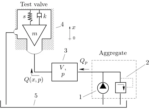
Figure 2 depicts a sketch of the analyzed system, which is similar to those used by Kasai [7] and Hayashi [6]. The system consists of a hydraulic aggregate and a safety valve connected by fluid conveying tubes, the fluid is redi-rected into an oil chamber after leaving the test valve. The oil is supplied by an aggregate that consist of the gear pump and an additional safety valve for the protec-tion of the system. This hydraulic aggregate provides the system the flow rate Qp. However, due to compressibil-ity of the fluid and elasticcompressibil-ity of the tubes, the flow rate at the test valve can be different from that one at the exit to the pump. To model the compressibility effects, a hypothetical chamber is added whose volume is equal to the total volume of oil in the system. This chamber will represent the stiffness of our system.
The mass balance equation for this chamber(labeled 3 in Fig. 2) can be written as follows:
d
dt(ρV) =ρ[Qp−Q(x, p)], (1)
0000 0000 0000 0000 1111 1111 1111 1111 0000 0000 0000 0000 1111 1111 1111 1111 00 00 11
11 000 0 0 0 0 0 0 1 1 1 1 1 1 1 1 1 00 00 00 00 00 00 11 11 11 11 11
1100000000001111111111
Aggregate V, Test valve 1 2 3 4 5 p s k m Qp
Q(x, p)
[image:2.595.309.547.69.243.2]0 x
Figure 2: Schematic diagram of a simple hydraulic sys-tem consisting of a gear pump (1), a relief valve (2), a hypothetical chamber (3) that represents the total tub-ing in a real system, the pressure relief valve (4) we wish to test and an oil tank (5).
where V represents the total volume of the system, ρ
denotes the density of the fluid andpis the oil pressure at the relief valve, Qp is the flow rate delivered by the pump and Q is the flow rate through the valve, which is a function of both the valve displacement x and the system pressurep:
Q(x, p) =A(x)Cd
r
2
ρp. (2)
Let us suppose that the valve is partly open. The flow-through area between the valve body and the seat will be calculated via the simplification that the normal dis-tancehof the cone to the valve seat (see Fig.3) is revolved around the symmetry axis of the cone along the circum-ference at an average radius. With these assumptions, we obtain
A(x) =dπh= (D−hcosα)πh,
wheredandDare defined in the figure andαis the semi-angle of the cone. With the substitution of h= xsinα
we finally obtain:
A(x) = (D−xsinαcosα)πxsinα=
(1−Dx sinαcosα)Dπxsinα. (3)
See Figure 3 for the geometry of the valve’s interior. With the assumption that the fluid is barotropic, i.e. its density depends only on the pressure, the left-hand side of Eq.(1) can be written as follows:
d
dt(ρV) =V dρ dt +ρ
dV dt =V
dρ dp
dp dt =V
ρ E
dp dt,
whereastands for sonic velocity: a2= dp dρ=
E
ρ. The
00000 00000 00000 00000 00000
11111 11111 11111 11111 11111
00000 00000 00000 00000 00000
11111 11111 11111 11111 11111 00000
11111
s k
m α
h
x
x
d D
[image:3.595.83.251.72.237.2]0
Figure 3: Geometry of the valve for calculation of the relationship between the efective orifice area A(x) and displacementx.
law, together with the usual impact law modelling the en-ergy loss of the impact via the restitution coefficient r. Finally, the system’s behaviour is described be the fol-lowing system of ordinary differetial equations (ODEs):
˙
x=v,
˙
v=pA
m − k mv−
s
m(x+x0), (4)
˙
p=E
V
Qp−A(x)Cd
r
2
ρp
and
v+=R v−=−rv−.
Herexandvdenote the displacement and velocity of the valve body, k is the damping coefficient,s is the spring stiffness, m is the total mass of the moving parts and
x0 denotes the pre-stress of the spring. Ais the area on which the fluid force originating from the pressure within the system acts,pdenotes the excess pressure in the sys-tem compared to atmospheric pressurep0(the pressure in the oil tank) andEis the reduced modulus of elasticity of the system after taking account of the oil compressibility and the expansion of the tubes. Qp denotes the oil flow rate generated by the gear pump,V is the overall volume of the system filled with oil. Cd(Re)is a discharge coef-ficient at the valve inlet which in general depends on the Reynolds number, although this dependence will be ne-glected in our subsequent analytical and numerical inves-tigation. A(x)denotes the effective orifice cross-sectional area when the valve is partly open andρis the density of the oil respectively. The expression of the orifice cross-sectional areaA(x)shown in Eq. (3) is very complicated so it is worth to linearise and write A(x) = c1x, where
c1 refers to the linear coefficient that describes the cross sectional area of the orifice as the function of the valve stem displacement. Since we experienced very small dis-placements during the experiments, the linearisation is believed to be an accurate approximation and so we can
restrict the nonlinearity to the third equation.
The last equation represents a simple impact law where
v− is the velocity before impact,v+ is the velocity after impact andris the coefficient of restitution.
2.1
Dimensionless equations
In order to treat the system in a more convenient way let us transform the equations into a non-dimensional form. We introduce the dimensionless variablesyi(τ)i= 1, ..,3, where:
τ = t
tref, y1= x
xref, y2= tref
xrefv, y3= p pref,
tref =
r
m
s, pref =p0 and xref = Ap0
s .
Eq.(4) can then be written in the nondimensional form
y′ 1=y2
y′
2=−κy2−(y1+δ) +y3 (5)
y′
3=β(q−√y3y1)
y2+=−ry−2,
where the nondimensional parameters are
κ= k
m
r
m
s (nondimensional damping coefficient)
β =E
V Cdc1A
ρ
r
2p0m
ρs (nondimensional stiffness param.)
δ= sxp
Ap0 (nondimensional pre-stress parameter)
q= Qp
Cdc1Aps0
q
2p0
ρ
(nondimensional flow rate).
Table 1 contains the physical parameters of the test rig
Par. Description Value
m mass of moving parts 0.45 [kg]
s stiffness of valve spring 15000 [N/m]
k damping coefficient 10-100 [N s/m]
p0 reference pressure 1e5 [P a]
A valve inlet cross section 1.767e-4 [m2]
E bulk modulus 0.435e9 [P a]
V total system volume 4.42e-4 [m3]
Cd discharge coefficient 0.86 [−]
ρ medium density 870 [kg/m3]
[image:3.595.308.548.511.646.2]c1 orifice opening parameter 0.0408 [m2]
Table 1: Physical parameters of the test rig used for cal-culation of the nondimensional parameters.
β = 19.5062 [−] andδ = 10 [−] corresponds to an open ing pressure of popening = 10 [bar] of the relief valve. From now on let us symplify the calculation and use
κ = 1.25 [−], β = 20 [−] and δ = 10 [−] instead. The nondimensional damping coefficient is only a rough ap-proximation as it is highly nontrivial how to estimate this parameter.
2.2
Linear stability analysis
When investigating dynamical systems we are inter-ested in finding equilibria and determining their stabil-ity. Therefore our first step will be to solve the governing equations when all the derivatives on the left-hand-side are zero. We then try to find cases when dynamical sta-bility loss occur, e.g. when self excited oscillations arise. In these cases a pair of complex conjugate eigenvalues of the system cross the imaginary axis with non-zero veloc-ity, e.g. their real part changes sign and become positive. We will search for a stability criterion using the system’s characteristic equation.
2.2.1 Equilibrium of the system
To calculate the equilibrium of the system we shall put the equations (5) in the form y′ =f(y) = 0. With the substitution√y3=z we obtain the following third order equation
z z2−δ−q= 0. (6)
We find that the real solution is
y1=y3−δ,
y2=0,
y3=
108q+ 12p−12δ3+ 81q22/3+ 12δ
2
36108q+ 12p−12δ3+ 81q22/3 .
For simplicity of the analytical calculations let us neglect the nondimensional prestress(δ= 0)so that the equilib-rium of Eq.(5) simplifies to
(y1e, y2e, y3e) = (q
2 3,0, q
2 3)
After linearisation around this equilibrium the Jacobian of the system is:
J =
0 1 0
−1 −κ 1
−βq13 0 −1
2βq
1 3
, (7)
which has the characteristic equation
λ3+a2λ2+a1λ+a0= 0, (8)
where a2=κ+12βq
1 3,a
1 = 1 +κβ12q
1 3 and a
0= 32βq
1 3.
Now let us to substituteλ= 0into Eq.(8) and conclude that steady stability loss (a fold bifurcation) can occur when following condition is true:
a0= 3 2βq
1 3 = 0.
Of course this case is meaningless, since β > 0 and we always assume a flow rate greater than zero.
We furthermore expect that the system undergoes a dy-namical stability loss, so now we substitute λ=iω into Eq.(8) in order to obtain the criteriona1a2=a0 for the Hopf-bifurcation. From this condition we can compute the curve of stability loss for the nondimensional damp-ing coefficient as the function of the nondimensional flow rate analytically:
κ= −β 2q2
3 −4 +
q
β4q4
3 + 40β2q 2 3 + 16
4βq13
(9)
Figure 4(a) shows the curve as a stability diagram. Here we substituted β = 1 into the equation above, results for other β values are qualitatively similar. The vibra-tion frequency at the critical points (i.e. on the curve) can also be derived from the same condition. We obtain
ω=√a1, wherea1is the coefficient ofλin the character-istic polinomial. With the transformation to dimensional coordinates we reach to the diagram shown in Figure 4(b) for the system’s vibration frequencies. Here we used pa-rameters that corresponds to the test equipment again (see Table 1). Figure 5. depicts the same stability dia-gram as 4(a) but in this case with physical parameters. We notice that the curve begins at the origin and has a local extremum (maximum) atQp = 0.05 [l/min]. If we assume, that our test valve can be characterized by a vis-cous damping coefficient ofk= 20[N s/m](marked with a red line on Fig.5) then the unstable region obtained from the diagram is below Qp ∼= 0.25 [l/min]. Here again we should mention that measuring the damping ratio is one of the most difficult tasks when investigating dynamical systems experimentally.
2.3
Nonlinear analysis
[image:4.595.55.287.422.549.2]q
κ
stable
unstable 0.75
0.4
0 25
(a)
Q
p[
l/min
]
f
[
H
z
]
frequency at314 [Hz] 300
0
0 3.5
[image:5.595.316.530.78.247.2](b)
Figure 4: Stability diagram for the nondimensional damping coefficient with respect to the nondimensional flow rate (a), the vibration frequency for the test system is expected to be at 314 [Hz] (b), using parameters in Table 1.
300
0
0 3.5
Qp[l/min]
k
[
N
s/
m
]
unstable
stable
Figure 5: Stability diagram for the laboratory test valve assumingk= 20 [N s/m](red line)
2.3.1 Normal form transformation
First we substituteχ=βq1/3into Eq. (7) to simplify the calculation. With this we can elliminate the parameterβ
from the equations. Now Eq. (7) can be written
J=
0 1 0
−1 −κ 1
−χ 0 −χ/2
. (10)
We next compute the three eigenvectors of the Jacobian that we will use for the linear transformation to appro-priate coordinates. They are
s1=
1
iω
1−ω2
−κiω
s2=
1
−iω
1−ω2
−κiω
s3=
1
−κ−χ/2
κχ/2 +χ2/4 + 1
.
These eigenvectors correspond to the case when two purely imaginary and one real eigenvalues exist. Specifi-cally: λ1=iω,λ2=−iωandλ3=−κ−χ/2.
The normal form transformation is a coordinate transfor-mation from the original coordinates (yi,i= 1...3in our case) to coordinates (ξ as they will appear later) laying on a polynomial approximation to the so-called centre manifold. The local dynamics of the system on the cen-tre manifold are then topologically equivalent to those in the phase space and so we can analyse stability by reduc-ing the number of coordinates from the three-dimensional space to the plane.
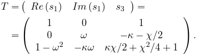
[image:5.595.305.538.508.586.2]of the form
T = Re(s1) Im(s1) s3 =
=
1 0 1
0 ω −κ−χ/2
1−ω2
−κω κχ/2 +χ2/4 + 1
.
Here the columns ofT represent the real and imaginary parts of the first and the real third eigenvector. Our aim by choosing the elements of the transformation matrix is to obtain a system with real parameters after the trans-formation.
Before being able to do the transformation it is simplest to replace all nonlinear equations with their third order Taylor expansion around the equilibrium to put the sys-tem into the following form
η′=Jη+p 3(η),
where J is the linear coefficient matrix, e.g. the Jaco-bian of the system and p3 contains all the higher order terms. Here we also consider small disturbances around the equilibrium and put therefore η = y −y0 into the equations.
The coordinate transformation is then following
η=T ξ, (11)
and the equation will have the form
T ξ′=AT ξ+p 3(T ξ).
We can write such a system in first order form as
ξ′=T−1AT
| {z }
B
ξ+H(ξ),
or more conveniently in matrix form
ξ′ 1 ξ′ 2 ξ′ 3 =
0 ω 0
−ω 0 0
0 0 −λ3
ξ1 ξ2 ξ3 +
H1(ξ)
H2(ξ)
H3(ξ)
.
(12) Note that elements of the nonlinear vector H(ξ) may contain any combination of products of the transformed coordinates.
2.3.2 Centre manifold reduction
A problem arises when we wish to apply normal form theory to our three-degrees-of-freedom system, since it is only applicable for systems of two degrees of freedom. Therefore we express the third coordinate ξ3 with the other two as a second-order Taylor series
ξ3=h11ξ12+h12ξ1ξ2+h22ξ22+O ξ3
(13)
We now need to find equations for the coefficientsh11,h12 andh22. The idea we will use is to compute the derivative
of Eq. (13) and make it equal to the third equation of our system in Eq. (12). Then we can express these coeffi-cients with those used for the third-order approximation of the nonlinear equation in the following way
2h11ξ1 ξ1′
|{z}
ωξ2
+h12(xi′
1ξ2+ξ1 ξ2′
|{z}
−ωξ1
) + 2h22ξ2ξ2′ =
=λ3 h11ξ21+h12ξ1ξ2+h22ξ22
+ +H311ξ12+H312ξ1ξ2+H322ξ22
| {z }
H3(ξ1,ξ2)
Here we can substituteξ′
1andξ2′ from the first two equa-tions of Eq. (12) as shown. This yields a linear system for the unknown vectorh= (h11h12h22)T
−λ3 −ω 0
2ω −λ3 −2ω
0 ω −λ3
h11 h12 h22 = H311 H312 H322
Now we know all the coefficients for the second order ex-pression of our third coordinateξ3that we can substitute into the first two equations of Eq. (12) and collect all the coefficients of the higher order terms. These we have to substitute into the so calledBautin formula [9] to obtain the value for the first Lyapunov coefficient. The formula we will use is as follows:
l(0) = 18ω1[(a20+a02) (−a11+b20−b02) + (b20+b02) (a20−a02+b11)] +18[3a30+a12+b21+ 3b03],
whereaijandbij(i+j= 2,3) are coefficients of the higher order terms in the transformed equations. If l(0) < 0 then the Hopf bifurcation is supercritical, e.g. a stable limit cycle is born, and ifl(0)>0then the bifurcation is subcritical and the limit cycle will be non-attracting.
[image:6.595.73.269.93.146.2]2.3.3 Results
Figure 6 shows the Lyapunov coefficient along the stabil-ity curve obtained by the linear analysis. Note that there is a change in the sign around κ = 0.67, below which the second Hopf bifurcation point will become subcriti-cal. Later we will present numerical continuation results showing this to be the case.
Now let we discuss further the values of the vibration fre-quency. As we obtained earlier in Section 2.2 there is an analytical expression for the frequency
ω=√a1=
s
1 +χ−χ
2−4 +pχ4+ 40χ2+ 16
8χ ,
whereχ=βq1/3.
The limits ofω for large and small flow rates are
lim
χ→0ω= 1 and χlim→∞ω= √
These analytical results are also clear to see in Figure 6. (Note the logarithmic scale on the figure.) This may sug-gest that the second Hopf point is quite far from the phys-ical flow rate values that correspond to a lower range ofχ. Now let we take a look at numerical continuation results
χ
κ
l
1ω
0 0 0
1 1 1
2 2 2
3 3 3
10 10 10 10 10 10 10
10 10 10 10 10 10 10
10 10 10 10 10 10 10
−1
−1
−1
−2
−2
−2
−3
−3
−3
1.2
1.4
1.6
1.8
0 0
0.2
0.4
0.6
0.8
−1
−2
1 1
2 x10
[image:7.595.315.532.81.257.2]−3
Figure 6: Stability curve (top), values of the Lyapunov coefficient along the stability curve (middle) and the vi-bration frequency (bottom) in logarithmic scale
for two different values of the damping coefficient. We used the programAUTO [3] (The program can be down-loaded from http://indy.cs.concordia.ca/auto/). Fig. 7 shows the numerical continuation with κ = 0.7, where since l(0) < 0 in this region we have two supercritical Hopf bifurcation points. The solid lines represent the data from the AUTO calculation and the dashed lines show the analytical estimation of the vibration ampli-tude. For this we used the following formula:
r≈
s
−σ
′
q(0)
l(0) (q−q∗),
whereris the vibration amplitude in the transformed co-ordinates, σ′
q(0)is the velocity at the critical point with
which the complex conjugate eigenvalues are crossing the imaginary axis andl(0)is the Lyapunov coefficient eval-uated at the critical parameter value. q is the nondi-mensional flow rate andq∗ is the flow rate at the critical point e.g. when we are on the stability curve. The cross-ing velocity σ′
q(0) was computed numerically by solving
q
y1
12
10
8
6
4
2
0
0 5 10 15 20 25 30
Figure 7: Continuation from the first Hopf point with
κ= 0.7. Both points are supercritical. The dashed lines represent the analytical estimation, and the solid lines the results of AUTO computation.
the characteristic equation and estimating the derivative from the difference between values at discrete points. Afterwards we transformedrback to the real coordinates with Eq. (11)
η=T
rsin(ωτ)
rcos(ωτ) 0
.
It is interesting to compare continuation diagrams with a reduced value of the damping coefficient in order to see, how the dynamics change around the critical points. Fig. 8 shows the neighborhood of the first Hopf bifur-cation point at q = 0.96 with κ = 0.4 . The stars mark the equilibria, circles represent the periodic solu-tions. Black markers are stable, red ones are unstable solutions. Here, the dashed line again shows the analyt-ical estimation from the bifurcation point. We can see, that the first bifurcation point is supercritical, however the periodic solution reaches a fold point and turns back as an unstable periodic solution. Aroundq= 0the con-tinuation stopped with the lack of convergence.
In Fig. 9 we can see the second Hopf point atq= 668.2 from which an unstable periodic solution arises. The sym-bols and colors on this figure have the same meaning as on Fig. 8. Note that this value of the nondimensional flow rate is unphysically high for a real hydraulic system, since q = 668.2 [−] = 14500 [. l/min] in the case of our particular test rig.
3
Global dynamics
[image:7.595.52.276.159.425.2]tech-nique enables us to study the global dynamics of the sys-tem.
3.1
Numerical simulation
Numerical simulation is a simple and effective method for analysing dynamical systems and can be one step of a deeper investigation. It also enables us to treat systems with discontinuity, e.g. when the solution trajectory or its derivative is non continuous in the phase space. Of course there are several issues that we should take into consider-ation in order to obtain accurate results. For example the type of ODE solver. There are numerous computer en-vironments that provide a numerical ODE solver such as some computer algebra packages or numerical mathemat-ical packages. We chose this latter environment since it provides a wide range of solvers with adjustable error tol-erance and gives us a convenient way to manipulate data and results using an effective programming language. It also enables us to use the so calledevent handling feature that is needed when treating impacting systems. We will use this for the detection of crossings with the Poincarè section as well.
In our simulation code we solve the nondimensional equa-tions. For this we use the physical parameters of the test rig mentioned earlier that was built up in the laboratory. Let us now present some results and in so doing explain some of the particular features of our implementation. Fig. 10(a) shows impacting solutions. The red solution line in the pressure plot is the equidistant qubic inter-polation of the solution that can be used for harmonic analysis. An example spectrum of the pressure solution of Fig. 10(a) is presented in Fig. 10(b). The pressure
q
y
13
0
[image:8.595.312.544.83.265.2]0 0.2
Figure 8: Continuation from the first Hopf point withκ= 0.4. The stable limit cycle is reaching a fold point, turns back an become unstable. The dashed line represents the analytical estimate.
q
y
10 1000
0 200
Figure 9: Continuation from the second Hopf point with
κ = 0.4 showing the unstable limit cycle. The dashed line represents the analytical estimation.
time history is not sinusoidal, so we find higher frequency components as well.
Now let us take a look at the phase space and see the sta-ble impacting limit cycle that exist for particular param-eters. This can be seen in Fig. 11. The nondimensional parameters here areq= 3,κ= 1.25,β = 20and δ= 10. Our program is capable of treating outer excitation in the form of an explicit time-dependent flow rate distur-bance around a given value. This can be useful when comparing numerical and experimental data. The rea-son of this feature comes from the experiments with the test rig. We experienced that the influence of the peri-odic excitation of our gear pump unfortunately cannot be neglected. Furthermore, we extended our program with the capability of producing so called brute force bifurca-tion diagrams that will be presented in the next secbifurca-tion. These diagrams basically show how trajectory crossings with a given Poincarè section changes when varying a parameter.
3.2
Numerical bifurcation diagrams
One of the earliest methods we can use during the inves-tigation of dynamical systems is to compute bifurcation diagrams numerically. This can be performed by solv-ing the set of equations with an appropriate ODE solver in forward time. We should choose a suitable Poincarè map in the phase space and let the solution trajectories be recorded when crossing this surface. Starting multiple iterations with random initial conditions for each value of the bifurcation parameter can lead us to the so called ‘Monte Carlo’ diagram.
[image:8.595.55.284.504.687.2]cho-t[s]
t[s]
t[s]
x
[
m
m
]
v
[
m
/
s
]
p
[
ba
r
]
0.9
0.9
0.9
1.1
1.1
1.1
0 0 0 4
−1 30
(a)
x 1010
f [Hz]
0 1000
0 3.5
[image:9.595.60.267.80.442.2](b)
Figure 10: A typical impacting solution of the system (a). Displacement (top), velocity (middle) and system pressure (bottom). The spectrum is depicted showing the vibration frequency and its higher harmonical com-ponents (b).
sen unless otherwise stated: κ= 1.25, β = 20, δ = 10,
r= 0.8. After an impact the velocity can be written as
v+=
−rv−. Herev−is the velocity before andv+after a particular impact. The bifurcation parameter (the nondi-mensional flow rate) was varied between q = 0.01−10 and for eachqthree random iterations were started from a30×20×80subset of phase space. Figure 12 shows the chosen Poincarè section in the phase space that is simply they2= 0plane.
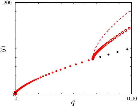
Now we should take a closer look at the results of the computation that can be seen in Figure 13. There are some interesting regions in the figure that should be dis-cussed. Let us consider reducing qfrom a high value to-wards zero. At aboutq= 9.18a stable limit cycle is born and it grows quick in amplitude with further decrease of the bifurcation parameter. This extreme growth can be explained from the fact that the first Lyapunov coefficient remains relative close to zero but is clearly negative for
y1 y2
y3
0 25
−5
5
0
[image:9.595.326.522.88.240.2]3
Figure 11: Impacting limit cycle for a nondimensional flow rate ofq= 3. The constant parameters areκ= 1.25,
β = 20andδ= 10.
Figure 12: Solution trajectories impacting at the y1 = 0 plane. The yellow plane depicts the chosen Poincarè section, they2= 0plane.
values ofqlower than aboutq∼= 17338as we obtained in subsection 2.3. A typical solution trajectory within this region is depicted in Figure 14(a).
At q ∼= 7.54 a grazing bifurcation occurs. This means that the amplitude of the vibration grows and reaches the impacting barrier y1 = 0 which means that the dis-placementxof the valve poppet has reached0, the value at the valve seat in our physical system. At grazing, only zero velocity impacts occur, this also means that the re-set map that is used for determining the velocity after impact is the identity map itself, the velocity before and after the impact are both equal to zero.
[image:9.595.317.531.333.488.2]be cloudy which is the hallmark of chaotic motion. Fig-ure 14(b) shows an impacting (weakly) chaotic solution. The next interesting point is atq∼= 5.9 where a period-two and a period-one impacting solution coexist. The period-two solution is an impacting/grazing one that can be seen in Figure 14(c). This also suggests that another grazing bifurcation occurs in this region when the non-impacting period of the period-two solution touches the impact surface.
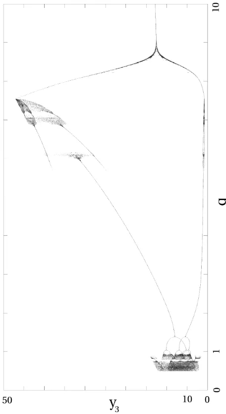
[image:10.595.54.282.267.685.2]Below q = 5.7 only a period-one impacting solution ex-ists until q= 1.4 where it is clear to see that a so called period-adding cascade starts. Figures 14(d), 14(e) and 14(f) show trajectories corresponding to this region. It is believed that this period adding ends up in the chaos that can be seen on Fig. 15(a). The region belowq= 0.5
Figure 13: Bifurcation diagram for variating the nondi-mensional flow rate q. The nondimensional pressure y3 is plotted against the bifurcation parameter. The other parameters are set toκ= 1.25,β = 20andδ= 10.
however remains unknown from Fig. 13. The behaviour of the system for these small flow rates is often called chattering. In case of chattering a series of impacts occur with less and less valve lift, just like the bouncing ball on a flat surface.
There are basically two types of chattering,completeand incomplete. At complete chattering an infinite number of impacts occur in finite time and the impacting part will come to a rest, it will stick. At incomplete chatter there is no sticking but the impacting body will begin to move for some reason. This can be a force, coming from the rising pressure under the valve poppet in our particular case and this force will lift the poppet again.
There are some issues when modelling the chatter phe-nomenon and our numerical simulator is not yet able to correctly describe this case and needs improvement. For example we shall consider that our simple impact law may not be valid in this region, when low velocity im-pacts are following each other quite quick. Also the flow characteristics through the narrowing orifice may change when the poppet is nearing the valve. The pressure will rise when the valve is almost closed and this can have an effect of an additional damping for the system.
All this issues shall be taken into consideration when we wish to investigate the valve’s behaviour at low flow rates. Producing numerical bifurcation diagrams is a very
y1 y2
y3
0 50
−10 10
6
(a)
y1 y2
y3
0 80
−10 20
−2
10
(b)
y1 y2
y3
0 60
−10 20
−2
8
(c)
y1 y2
y3
0 40
−10 10
−1
5
(d)
y1 y2
y3
2 14
−4 4
−0.2
1
(e)
y1 y2
y3
0 15
−4 4
−0.5
1
(f)
[image:10.595.322.525.398.675.2]y1 y2
y3
0 20
−4
4
−0.5
1
(a)
f[Hz]
0 200 800 1000
x108
0 2 4 6 8
(b)
Figure 15: (a) Chaotic attractor for q ≈0.85 with κ = 1.25,β = 20andδ= 10. (b) The frequency spectrum of the solution.
powerful method because these results can give a brief overview of the system’s global behaviour. In the next section we will focus on the investigation of the grazing bifurcation that occurs when the response of the system first becomes impacting.
4
Grazing bifurcation analysis
Strong nonlinearities in a dynamical system such as im-pacts can have serious and sometimes unexpected effects. It sometimes can happen for example that a stable pe-riodic motion will suffer a sudden jump to chaos or at least period adding can be observed. In this section we will use techniques described in [2] to understand more from the discontinuity-induced bifurcations occuring due to grazing of our pressure relief valve with the valve seat.
4.1
Grazing events
In our system for the particular nondimensional param-eters used (κ= 1.25,β = 20,δ = 10) grazing can occur at two flow rates that are q = 7.54 and at q = 5.95. The first occurrence is when the period-one nonimpact-ing limit cycle depicted in Fig. 14(a) touches the impact barrier. The other case is when a period-two limit cycle that already has an impacting period undergo a second grazing (see Fig. 14(c)). In both cases this is
character-q
y3
6.6 8.2
34 48
(a)
q
y3
4.5 7
26 38
[image:11.595.71.271.84.451.2](b)
Figure 16: Two grazing events shown in the bifurcation diagram. The first a t q = 7.54 (a) and the second at
q= 5.95(b).
[image:11.595.322.521.231.624.2]4.2
Bifurcation scenario at grazing
We carried out an analytical investigation for the first case (where q = 7.54) to find out what type of grazing bifurcation we have to deal with. For this we used the theory for nonsmooth systems described in [2]. First we have to find the grazing limit cycle exactly. Our bifurca-tion diagram in Fig.13 is very helpful, because it contains the critical flow rate q and the nondimensional pressure
y3can also be obtained. Since we chose the zero velocity plane as our Poincarè sectiony2= 0 and at grazing our displacement is also zero. We now have initial conditions that correspond to the last non-impacting limit cycle. The next step is to solve the so called linear variational equations along the limit cycle, to obtain themonodromy matrix. These equations can be written in following form:
˙
w= ˆJw, (14)
whereJˆis the linear part of the nonlinear system defined in Eq. (5) but without substituting the equilibrium. So (14) can be written in the form:
˙
w1 ˙
w2 ˙
w3
=
0 1 0
−1 −κ 1
−β√y3 0 −12√βyy1
3
w1
w2
w3
,
and Jˆ is linear with respect to w. We have to solve (14) together with the system’s equations for the period
T of the grazing limit cycle three times with the initial conditions w01
1 , w012 , w301
= (1,0,0), w02
1 , w022 , w302
= (0,1,0)and w03
1 , w032 , w303
= (0,0,1). We can then com-pose the monodromy matrix M from the solutionw(T) after one complete period in following way:
M = w01(T)w02(T)w03(T)
We now have to compute the eigenvalues ofM and apply the theory described in [2].
For the grazing flow rate q = 7.54 we can find
y0 1, y02, y03
(0,0,47.07) as initial condition of the graz-ing limit cycle. When we integrate for one period (T = 2.6547for this flow rate) and solve the linear variational equations we obtain that
M =
0.5972 0.0450 −0.0111 13.4466 1.5311 −0.1306 40.8328 5.1828 −0.2744
,
whose eigenvalues areν1= 1,ν2= 0.8537andν3= 0. It is necessary to have one eigenvalue that is equal to1. ν3 does not necessarily have to be zero, but presumably it is close to and the difference may be beyond the compu-tation tolerance.
The second eigenvalue gives us important information about the scenario after the grazing event. First of all it has to be less than1because the grazing limit cycle is attracting, e.g. it is stable.
According to theory there are three scenarios:
1. If 0< ν <1/4then grazing is followed by a period adding, in which the periodic bands overlap,
2. if 1/4 < ν < 2/3 then chaotic and stable periodic solutions are alternating and periodic motion forms a period adding cascade,
3. if2/3< ν <1 then there is a sudden jump to chaos to obtain, and the chaotic attractor’s size is square root proportional to the bifurcation parameter.
Since we have 2/3 < ν2 < 1, a robust chaotic attractor arises, as it can also be seen in Fig. 16(a). It is also easy to notice that it is growing like a square root function. According to literature [2] this behaviour is characteristic to impacting systems. Note that this approach is only valid if we assume that the discontinuity map has quasi one-dimensional behaviour. The literature [2] contains lots of examples and presents various bifurcation dia-grams, also ones that refer to the other two scenarios. An example figure for the first case, e.g. when 0< ν <1/4 looks very similar to our second grazing scenario that arises atq= 5.95. This could be analysed with the same technique in a latter investigation.
4.3
The three-dimensional square root map
Impacting systems have a so called square root-type non-linearity. This means that the bifurcation scenario that occur at grazing can be described by a square root map. Such a map can be written in general form
x7→M x+N µ+Ey,ifH(x, µ)<0, (15)
and
x7→M x+N µ,ifH(x, µ)>0.
M is the monodromy matrix mentioned earlier, N is a column vector that is obtained by the same linear vari-ational equations as the matrix M but we have to add the partial derivative with respect to the bifurcation pa-rameter. In our case this only means the addition ofβ to the third equation since ∂y′3
∂q =β. At this time we have
to solve the equations around the grazing periodic orbit with the initial conditions(0,0,0). In our particular case we obtain
N = (0.2269−0.1939−7.3400)T.
H(x, µ)
v x1
x2 x3
[image:13.595.317.525.78.244.2]x4
Figure 17: The ZDM maps in practice. The pointx1 is mapped to the pointx4in which the solution is integrated backward time fromx3for the time that elapsed between the pointsx1 andx2.
point arbitrary close to the grazing point and integrating it forward in time until we stop at the impact surface and measure the elapsed time. Then we apply the impact law but this time we integrate backward in time for the same time period that was recorded. See Fig.17 that shows an impacting trajectory together with the important points. For our investigation we will use following analytical ap-proach of the ZDM that can be found in [2]
x7→M x+N µ,ifH(x, µ)>0and
x7→M x+√2a∗W(x)y+N µ,ifH(x, µ)<0,
where a∗ is the acceleration at the graing point, W(x) contains the coefficient of restitution, µ = q−qcrit is the bifurcation parameter and y =√−x represents the square root singularity. In our particular case we can substitute
a∗=p∗−δand
W(x) =
0 1 +r
0
,
where p∗ is the grazing pressure. Next we iterate the three dimensional map and produce bifurcation diagrams by varying the bifurcation parameter. We varied q be-tween 7.4 and7.6 and obtained the bifurcation diagram for the map presented in Fig.18. It is clear to see that a chaotic attractor arises immediately after grazing. Note that the lower and upper boundaries of the chaotic at-tractor show linear and square root type shape that is characteristic to impacting systems and the upper square root shaped boundary is proportional to√µaccording to [2].
5
Conclusions
In this paper we presented a mathematical analysis of a simple hydraulic pressure relief valve. We found that
q
y
7.4 7.65
−0.1 0.25
Figure 18: Bifurcation diagram of the three-dimensional ZDM betweenq= 7.4−7.6. yis the second coordinate of the map. A sudden jump to chaos can be observed at the critical flow rateqcrit= 7.54. The dashed line represents the analytical estimation.
these kind of dynamical systems can lose their stability in a particular way in which self-excited limit cycle vi-brations occur. We obtained a criterion for stability re-garding the flow rate and damping coefficient parameters using linear stability analysis. We have shown that damp-ing of the system has a notable effect on the stability of arising limit cycle.
We also found that for low enough damping, the periodic orbit born in the Hopf bifurcation reaches the valve seat and the system undergoes a grazing bifurcation, with an immediate jump to chaos. We believe that this is the first description of this scenario corresponding to the onset of valve chatter as most previous studies assumed smooth behaviour, and essentially has just found the presence of Hopf bifurcations. As we have shown, the analysis of chatter requires nonsmooth dynamical systems theory.
For very small flow rates, another interesting phenomena occur: as the pressure in the system builds up very slowly, the valve body closes completely, which gives rise to stic-ing motion. In this case not only impact occurs but for some time intervals (while the valve is shut), the dynam-ics reduces simply to the pressure dynamdynam-ics with x= 0 and v = 0. Our future plan is to analyse this hybrid motion consisting of sticking, impacting and freely os-cillating segments. Obviously, laboratory measurements are also needed to verify the theoretical and numerical results.
Acknowledgements. This work was partially
[image:13.595.78.266.78.213.2]References
[1] W. Bolton. Pneumatic and hydraulic systems. Butterworth-Heinemann, 1997.
[2] M. di Bernardo, C. J. Budd, A. R. Champneys, and P. Kowalczyk.Piecewise-smooth dynamical systems. Springer, 2007.
[3] E. J. Doedel, R. C. Paffenroth, A. R. Champneys, T. R. Fairgrieve, Y. A. Kuznetsov, B. E. Oldeman, B. Sanstede, and X. Wang. AUTO 2000 : Continu-ation and BifurcContinu-ation Software for Ordinary Differ-ential Equations, 2006.
[4] J. Guckenheimer and P. Holmes. Nonlinear oscilla-tions, dynamical systems, and bifurcations of vector fields. Springer, 1983.
[5] S. Hayashi. Instability of poppet valve circuit.JSME International Journal, 38(3), 1995.
[6] S. Hayashi, T. Hayase, and T. Kurahashi. Chaos in a hydraulic control valve. Journal of fluids and structures, (11):693–716, 1997.
[7] K. Kasai. On the stability of a poppet valve with an elastic support. Bulletin of JSME, 11(48), 1968.
[8] F. X. Kay.Pneumatics for industry. The Machinery Publishing Co. Ltd., 1959.
[9] Yuri A. Kuznetsov. Elements of applied bifurcation theory. Springer, 1997.
[10] H. L. Stewart. Hydraulic and pneumatic power for production. The Industrial Press, 1963.


![Figure 5: Stability diagram for the laboratory test valveassuming k = 20 [Ns/m] (red line)](https://thumb-us.123doks.com/thumbv2/123dok_us/388799.536404/5.595.316.530.78.247/figure-stability-diagram-laboratory-test-valveassuming-ns-line.webp)