Online Full Text

Abstract—In recent years, fairness has been

increasingly emphasized in supply chain management studies. However, the existing literature focuses on its effect in non-cooperative environment. We innovatively incorporate fairness into cooperative supply chain, and investigate how it affects the firms’ optimal decisions and profits. Our results enable an efficient search for the firms’ optimal decisions. They also show that fairness concern of the manufacturer can promote demand, while fairness concern of the retailer can lower demand. In addition, when fairness concern of one firm is introduced into cooperative supply chain, an increase in its bargaining power can alleviate double marginalization effect. We conduct an extensive numerical study and find that introducing fairness concern of one firm into cooperative supply chain can increase that firm’s profit but decrease the other firm’s profit. Our numerical study also provides some insights on how the firms’ decisions and profits change with important factors such as fairness parameters and demand elasticity parameters.

Index Terms—Fairness, Cooperative supply chain,

Fairness preference factor, Elasticity of demand

I. INTRODUCTION

RADITIONAL economics theory research is based on the pursuit of self-interest. In the past decades, the introduction of behavioral science that is represented by prospect theory has proved the existence of behavior preference in economics [1], which is inconsistent with traditional theories. With the development of experimental economics, some researchers have shown the existence and importance of fairness preference. They attempt to apply fairness preference to explain the economic phenomena deviating from reality.

Researches in economics and marketing show that fairness plays an significant role in developing and maintaining channel relationship [2]-[3]. It is also important to introduce the fairness concept into supply chain management research. Supply chain collaboration is viewed as a business process where two or more partners work together toward common goals [4]-[5], and it is a common practice in various industries. However, among the existing literature, few papers study how fairness influences the cooperative supply chain. This paper is to fill the gap and

This work was partially supported by the National Natural Science Foundation of China, under Grant no.71601056.

L. Wang, Harbin Institute of Technology, Shenzhen, Shenzhen 518055, China (e-mail: [email protected]).

T. Xiao, corresponding author, Harbin Institute of Technology, Shenzhen, Shenzhen 518055, China (e-mail: [email protected]).

Q. Lu, Harbin Institute of Technology, Shenzhen, Shenzhen 518055, China (e-mail: [email protected]).

investigate the role of fairness in the cooperative supply chain.

We consider a supply chain with a manufacturer and a retailer, where the manufacturer determines the order quantity (lot size) and the retailer determines the retail price and the marketing expenditure. As pointed out by Esmaeili et al. (2009) [6], in many large industries with high production cost, it is common that the sellers decide lot sizes. In addition, many business relationships are long-term, and the manufacturer may charge the retailer a fixed wholesale price. We successively formulate and analyze the decentralized supply chain (Model B), the cooperative supply chain (Model C), the cooperative supply chain with fairness-concerned retailer (Model FR) and the cooperative supply chain with fairness-concerned manufacturer (Model FM). The analytical results allow us to conduct a one-dimensional search for the optimal lot size for solving each model. Given lot size, we compare the retailer’s decisions and induced demand in different models. In particular, we find that fairness concern of the retailer in cooperative supply chain leads to a lower demand compared with the case without fairness concern, whereas fairness concern of the manufacturer in cooperative supply chain leads to a higher demand. We also show that when fairness concern of one firm is introduced into cooperative supply chain, an increase in its bargaining power can alleviate double marginalization effect.

We conduct an extensive numerical study to illustrate the results and to obtain more insights. Introducing fairness concern of one firm into cooperative supply chain can increase that firm’s profit but decrease the other firm’s profit. The higher fairness concern of that firm, the more benefit he can earn. Our numerical study also shows that as demand elasticity parameters change, the trends of the optimal decisions and profits are similar in Models FR, FM and C. The retailer’s profit decreases as price elasticity of demand increases or marketing expenditure elasticity of demand decreases. However, the manufacturer’s profit is decreasing in marketing expenditure elasticity of demand, and it is not monotone in price elasticity of demand. In addition, our numerical study illustrates that as the retailer’s bargaining power becomes larger, the retailer’s profit increases, whereas the manufacturer’s profit decreases.

The remainder of this paper is organized as follows. Section Ⅱ reviews the literature on fairness and cooperative supply chain. Section Ⅲ provides the model description and some preliminary analysis. Section Ⅳ analytically compares the firms' decisions in different models. Section Ⅴ presents the numerical study. Section Ⅵ offers concluding remarks.

II. LITERATURE REVIEW

The Role of Fairness in Cooperative Supply

Chain

Lirong Wang, Tingting Xiao, Qiang Lu

*

T

IAENG International Journal of Applied Mathematics, 48:3, IJAM_48_3_05

Our paper is related to two streams of literature: one is fairness, especially in supply chain management, and the other is cooperative supply chain. The fairness generally has two types: one is reciprocal fairness, and the other is inequity aversion. Reciprocal fairness judges fairness by perceiving kindness and unkindness of behavioural intentions. Rabin (1993) [7] constructs an economic model involving fairness intention. The optimal response function depends on not only each other’s strategic options but also his second order faith. Participants judge each other’s kindness according to the comparison between their own real benefits and expected fair benefits. The inequity aversion considers the relative consistency of investment and giving. Thus, people have a tendency of disgusting inequity. In such a model, participants care about the fairness of results but not the intentions of each other. Fehr and Schmidt (1999) [8] define the fairness as the inequity aversion. The utility function of a player is divided into three parts: absolute income utility, jealousy preference negative utility and sympathy preference negative utility. Bolton and Ockenfels (2000) [9] propose another inequity aversion model called ERC (equity, reciprocity and competition), where the participants focus on their own profits and the relative level of total profit. Following the work by Fehr and Schmidt (1999), we consider the distributional fairness between the supply chain members.

As the pioneering work of incorporating fairness concern in supply chains, Cui et al. (2007) [10] investigate how the fairness may affect channel coordination. They find that the wholesale price contract can coordinate the supply chain. Based on Cui et al. (2007), Caliskan-Demirag et al. (2010) [11] analyze the case of nonlinear demand and extend the scope of the wholesale price contract. However, the demand hypothesis is deterministic so that the inventory decision-making problem can be ignored. Du et al. (2010) [12] and Ma (2011) [13] consider uncertain demand and assume that the retailer is fairness-concerned. The former shows that the fairness concern cannot change the status of supply chain coordination, while the latter considers the fairness concern as the retailer’s bargaining power for supply chain profit. Ho et al. (2014) [14] consider a supply chain with one supplier and two retailers, and study both peer-induced fairness concern and distributional fairness concern. Choi and Messinger (2016) [15] incorporate fairness into a competitive supply chain with two manufacturers and one retailer, and mainly derive their results from experiments.

Our paper is also related to the stream of literature on cooperative supply chain. Wang et al. (2004) [16] design a game-theoretical cooperative mechanism for a two-echelon decentralized supply chain. Several Nash equilibrium contracts are designed in echelon inventory games and local inventory games. Nagarajan and Sošić (2008) [17] survey some applications of cooperative game theory to supply chain management. They emphasize the profit allocation and stability of the cooperative game. Leng and Parlar (2009) [18] construct a three-person cooperative game including one manufacturer, one distributor and one retailer, and discuss a distributional cost problem when the three firms share the demand information. They obtain a unique distributional scheme. Cao and Zhang (2011) [19] study the nature of supply chain cooperation and its impact on firm

performance. Kawakatsu et al. (2013) [20] analyze the optimal quantity discount policy in cooperative supply chain and compare the cooperative case and the non-cooperative case. However, the influence of fairness concern on the firms’ decisions is not negligible in the process of cooperation. In this paper, we incorporate fairness into the cooperative supply chain and investigate the role of fairness in cooperative environment.

III. MODEL AND PRELIMINARY ANALYSIS

We consider a supply chain where a manufacturer sells a product to a retailer, who in turn sells the product to the consumer market. The manufacturer charges a fixed wholesale price (denoted by W), and he determines the lot size (denoted by Q). Based on Lee and Kim (1993) [21] and Esmaeili et al. (2009) [6], the annual demand is described by the following function.

D=kP−αEβ,

where P is the retail price charged by the retailer, E is the marketing expenditure per unit incurred by the retailer, k is the scaling constant for demand function,

α

is price elasticity of demand, and

β

is marketing expenditure elasticity of demand. We assume that k>0, 0< <β 1 and

1

α > +β . The retailer determines the values of the retail price P and the marketing expenditure E. Other parameters are listed as follows.

h percent inventory holding cost scale per unit per year,

r

O retailer’s ordering cost per order,

m

O manufacturer’s setup (ordering) cost per setup,

m

C manufacturer’s production cost per unit.

We assume that the manufacturer’s setup cost is higher than the retailer’s, that is, Om>Or. We also assume that the

production rate is equal to the demand rate, so there is no shortage.

In the following, we study the models of a decentralized supply chain and a cooperative supply chain respectively. We also incorporate the fairness concern into the cooperative case, and investigate the role of fairness in the cooperative supply chain. Thus, we totally consider three models, and denote them by Models B, C and F respectively.

A. Decentralized Supply Chain (Model B)

The sequence of events in the decentralized supply chain model is as follows. First, the manufacturer decides the lot size. Secondly, the retailer decides the retail price as well as the marketing expenditure.

Given the lot size Q, the retailer’s problem is to maximize her profit by determining the retail price P and the marketing expenditure E. Similar to Lee and Kim (1993) [21] and Esmaeili et al. (2009) [6], the retailer’s profit is the difference between sales revenue and total cost, where total cost includes purchase cost, market cost, ordering cost and holding cost. That is,

(

)

1

,

2

r r

D

P E PD WD ED O hWQ

Q

P = − − − − . (1)

Substituting the demand function into (1), we obtain

(

)

1

, .

2

r r

O

P E kE P P W E hWQ

Q

β −α 

P = _ − − − _−

 

IAENG International Journal of Applied Mathematics, 48:3, IJAM_48_3_05

According to the first order condition, we have

1

( ) , 1

B W O Qr

E β

α β

−

+ =

− − (2)

(

1

)

. 1

r

B W O Q

P α

α β

−

+ =

− − (3)

It can be shown that the above solution (PB_{(Q), E}B_{(Q) ) is}

optimal and unique.

The manufacturer’s problem is to maximize his profit by determining the lot size Q. His profit is the difference between sales revenue and total cost, where total cost includes production cost, setup cost and holding cost. That is,

( )

1

2

m m m m

D

Q WD C D O hC Q

Q

P = − − − . (4)

Substituting the demand function into (4), the manufacturer’s problem can be expressed as follows.

( )

(

1

)

1 1 ) , 2 , 1 ( ) . 1 ( m

m m m

r

r O

Max Q kP E W C hC Q

Q

W O Q

subject to P

W O Q

E α β α α β β α β − − −

P = − − −

+ = − − + = − − (5)

The optimal lot size, denoted by QB_{, can be found with}

optimization algorithms such as ant colony algorithm[22].

B. Cooperative Supply Chain (Model C)

In the cooperative supply chain, the manufacturer and the retailer jointly determine the lot size Q, the retail price P and the marketing expenditure E to maximize the weighted sum of their profits, that is,

(1 )

r m

r r

P = P + − P .

where r ∈

( )

0,1 can be considered as a measure of their bargaining powers, and Pr and Pm are given by (1) and (4)

respectively.

According to the first order condition, we have the following equations.

2 ((1 ) )

((1 ) )

m r

m

kP E O O

Q

h C W

α β _{r r}

r r

− _{− +}

=

− + , (6)

1 1

( ( ) (1 )( ))

( 1)

r m m

W O Q W C O Q

P α r r

r α β

− −

+ − − − − =

− − , (7)

1 1

( ( ) (1 )( ))

( 1)

m

r m

W O Q W C O Q

E β r r

r α β

− −

+ − − − − =

− − . (8) The optimal solution, denoted by (QC_{, P}C_{, E}C_{), can be}

found using iterative methods.

C. Cooperative Supply Chain with Fairness Concern

(Model F)

Now in the cooperative supply chain, we take into account fairness concern and investigate its effects in two cases. In the first case, only the retailer is inequity averse. In the second case, only the manufacturer is inequity averse. For convenience, we denote the two cases by Models FR and FM respectively.

Similar to Loch and Wu (2008) [23] and Du, et al. (2010) [12], we assume that the sensitiveness to gain and the sensitiveness to loss are the same for a player, which we call choice consistency. To formulate the utility function of a fairness-concerned player, we introduce the fairness

preference factor, which measures the sensitiveness to gain or loss.

In the first case, the retailer is inequity averse and the manufacturer is fairness neutral. Their utility functions are respectively

U_r = P −_r f_r,

m m

U = P ,

where f_r = P − Pa( _{m r}) . Here P − Pm r is the profit

difference between the manufacturer and the retailer, and

a>0 is the fairness preference factor of the retailer. When

a=0, the retailer is fairness neutral, and the problem becomes Model C.

The manufacturer and the retailer jointly maximize

(

1

)

(

1

)

(

1

)

r m r m

U =rU + −r U =r + P + − −a r ra P .

According to the first order condition, we obtain the following equations.

2 ((1 ) (1 ) )

((1 ) (1 ) )

m r

m

kP E a O a O

Q

h a C a W

α β _{r r r}

r r r

− _{− − + +}

=

− − + + , (8)

1 1

( (1 )( ) (1 )( ))

(1 )( 1)

m

r m

a W O Q a W C O Q

P

a

α r r r

r α β

− −

+ + − − − − − =

+ − − , (9)

1 1

( (1 )( ) (1 )( ))

(1 )( 1)

m

r m

a W O Q a W C O Q

E

a

β r r r

r α β

− −

+ + − − − − − =

+ − − . (10)

The optimal solution, denoted by (QFR, PFR, EFR), can be found using iterative methods.

In the second case, the retailer is fairness neutral and the manufacturer is inequity aversion. Their utility functions are respectively

r r

U = P ,

Um = P −m fm,

where f_m = P − Pb( _{r m}) . Here P − Pr m is the profit

difference between the retailer and the manufacturer, and

b>0 is the fairness preference factor of the manufacturer. When b=0, the manufacturer is fairness neutral, and the problem becomes Model C.

The manufacturer and the retailer jointly maximize

(

1

)

(

)

(1 ) 1

(

)

r m r m

U=rU + −r U = r+br− P + −b r + Pb . According to the first order condition, we obtain the following equations.

2 (( ) (1 )(1 ) )

Q

(( ) (1 )(1 ) )

r m

m

kP E b b O b O

h b b W b C

α β _{r r r}

r r r

− _{+ − + − +}

=

+ − + − + , (11)

1 1

(( )( ) (1 )(1 )( ))

( )( 1)

m

r m

b b W O Q b W C O Q

P

b b

α r r r

r r α β

− −

+ − + − − + − − =

+ − − − ,(12)

1 1

(( )( ) (1 )(1 )( ))

( )( 1)

m

r m

b b W O Q b W C O Q

E

b b

β r r r

r r α β

− −

+ − + − − + − −

=

+ − − − . (13)

The optimal solution, denoted by (QFM_{, P}FM_{, E}FM_{), can be}

found with iterative methods. IV. DISCUSSION

Based on the analysis in Section Ⅲ, for each model, we can express the optimal retail price and marketing expenditure as functions of lot size and conduct a numerical search for the optimal lot size. In this section, given the lot size Q, we compare the retailer’s pricing and marketing decisions in different models.

First, by comparing Model B and Model C, we obtain the following proposition.

IAENG International Journal of Applied Mathematics, 48:3, IJAM_48_3_05

Proposition 1: Given the lot size Q, both the retail price and the marketing expenditure in cooperative supply chain are respectively lower than those in decentralized supply chain.

Proof. Comparing (2) and (3) with (7) and (8), we can obtain

1

(1 )( ) ( 1)

B C W Cm O Qm

P P

α

r

r α β

−

− − −

− =

− − ,

1

(1 )( ) ( 1)

B C W Cm O Qm

E

E

β

r

r α β

−

− − −

− =

− − .

The manufacturer will never make negative profit, so we haveW Cm O Qm 1 0

−

− >

− . Then the above two equations are greater than 0. That is, B C

P >P , B C

E >E . The proof of Proposition 1 is completed.

Proposition 1 shows that the retail price and the marketing expenditure decrease when the supply chain members cooperate. While cooperation alleviates double marginalization effect, it also reduces the retailer’s incentive to expend marketing effort. These may lead to conflicting effects on the induced demand. We can further show the following corollary.

Corollary 1: The demand in cooperative supply chain is higher than that in decentralized supply chain.

Proof. The demand in cooperative supply chain and decentralized supply chain are respectively

( ) ( )

B B B

D =k P −α E β and DC =k P( C)−α(EC)β . Moreover,

/ / /

B B C C

P E =P E =α β.Thus, DB =k( /α β)−α(EB)− +α β,

( / ) ( )

C C

D =k α β −α E − +α β. According to Proposition 1, we

have B C

E >E . In addition, α β> . Therefore, we can obtain B C

D <D . The proof of Corollary 1 is completed. Corollary 1 implies that the cooperation between the retailer and the manufacturer can promote demand increase and contribute to the market development. Therefore, the firms may tend to cooperate with each other, so that the supply chain as a whole can have a competitive advantage.

Now we compare Model C and Model F, and obtain the following proposition.

Proposition 2: Given the lot size Q, the retailer’s decisions in cooperative supply chain have the following properties when fairness concern is considered.

(1) When the retailer is fairness-concerned, both the retail price and the marketing expenditure are higher than those in the case without fairness concern.

(2) When the manufacturer is fairness-concerned, both the retail price and the marketing expenditure are lower than those in the case without fairness concern.

Proof. (1) Comparing (7) and (8) with (10) and (11), we can obtain

(

(1

)(

1

)

)

FR C a W Cm Om Q

P P

a

α

r

α β

− −

− =

+ − − ,

( )

(1 )( 1)

FR C a W Cm Om Q

E E

a

β

r

α β

− −

− =

+ − − .

Since W Cm O Qm 1 0

−

− >

− , the above two equations are greater than 0. Thus result (1) holds.

(2) Comparing (7) and (8) with (13) and (14), we can obtain

1

( )

( )( 1)

FM C b W Cm O Qm

P P

b b

α

r r r

α β

−

− − −

− =

+ − − − ,

1

( )

( )( 1)

FM C b W Cm O Qm

E E

b b

β

r r r

α β

−

− − −

− =

+ − − − .

Since W Cm O Qm 1 0

−

− >

− , the above two equations are less than 0. Thus result (2) holds. The proof of Proposition 2 is completed.

When the retailer is fairness-concerned, the cooperative supply chain charges a higher retail price and expends more marketing effort, which may lead to higher profit for the retailer. When the manufacturer is fairness-concerned, the cooperative supply chain charges a lower retail price to further alleviate double marginalization effect, which may lead to higher profit for the manufacturer. However, in this case, the cooperative supply chain reduces the retailer’s incentive to expend marketing effort. We can further have the following corollary.

Corollary 2: The demand in cooperative supply chain with fairness-concerned retailer is lower than that in the case without fairness concern. On the contrary, the demand in cooperative supply chain with fairness-concerned manufacturer is higher than that in the case without fairness concern.

Proof. The proof is similar to that of Corollary 1.

Thus, fairness has a significant influence on the market. In cooperative supply chain, the market demand decreases when the retailer considers fairness, and it increases when the manufacturer considers fairness. Combining Corollaries 1 and 2, we have that fairness concern of the manufacturer in cooperative supply chain can further promote the market demand and stimulate social economy development.

The results in the above two propositions and corollaries are summarized in Table Ⅰ.

Table Ⅰ Comparison results

P E D

B vs. C B C

P >P B C

E >E B C

D <D

FR vs. C FR C

P >P FR C

E >E FR C

D <D

FM vs. C FM C

P <P FM C

E <E FM C

D >D

In the supply chain relationship, the members’ bargaining powers have vital effects on decisions making [24]. We now study how the bargaining powers of the manufacturer and the retailer affect the retailer’s price and marketing decisions in different models.

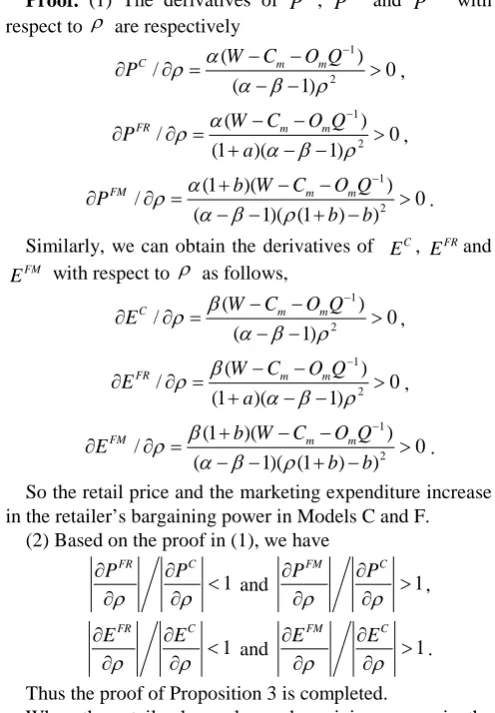
Proposition 3: Given the lot size Q, the retailer’s decisions in cooperative supply chain have the following properties.

(1) The retail price and the marketing expenditure increase in the bargaining power of the retailer no matter whether fairness is concerned.

(2) When the retailer is fairness-concerned, the sensitivity of the retailer’s decisions with respect to her bargaining power is lower than that in the case without fairness concern. When the manufacturer is fairness-concerned, the sensitivity of the retailer’s decisions with respect to her bargaining power is higher than that in the case without fairness concern.

IAENG International Journal of Applied Mathematics, 48:3, IJAM_48_3_05

Proof. (1) The derivatives of _PC _{, P}FR _{and P}FM _with

respect to r are respectively

1 2 ( ) / 0 ( 1) m

C W Cm O Q

P

r

α

α β

r

−

− −

∂ ∂ = >

− − ,

1

2

( )

/ 0

(1 )( 1)

FR W Cm O Qm

P

a

α

r

α β

r

−

− −

∂ ∂ = >

+ − − ,

1

2

(1 )( )

/ 0

( 1)( (1 ) )

FM b W Cm O Qm

P

b b

α

r

α β

r

−

+ − −

∂ ∂ = >

− − + − .

Similarly, we can obtain the derivatives of C

E , FR

E and

FM

E with respect to r as follows,

1 2 ( ) / 0 ( 1) m

C W Cm O Q

E

r

β

α β

r

−

− −

∂ ∂ = >

− − ,

1

2

( )

/ 0

(1 )( 1)

FR W Cm O Qm

E

a

β

r

α β

r

−

− −

∂ ∂ = >

+ − − ,

1

2

(1 )( )

/ 0

( 1)( (1 ) )

FM b W Cm O Qm

E

b b

β

r

α β

r

−

+ − −

∂ ∂ = >

− − + − .

So the retail price and the marketing expenditure increase in the retailer’s bargaining power in Models C and F.

(2) Based on the proof in (1), we have

1

FR C

P P

r

r

∂ ∂ _<

∂ ∂ and 1

FM C

P P

r

r

∂ ∂ _>

∂ ∂ ,

1

FR C

E E

r

r

∂ ∂ _<

∂ ∂ and 1

FM C

E E

r

r

∂ ∂ _>

∂ ∂ .

Thus the proof of Proposition 3 is completed.

When the retailer has a larger bargaining power in the supply chain, she may increase her retail price and marketing expenditure to improve her own profit. In addition, when one firm is fairness-concerned, the changes of the retail price and marketing expenditure with respect to its bargaining power are respectively slower than those in the case without fairness concern. Thus, when fairness concern of one firm is introduced to cooperative supply chain, an increase in its bargaining power can alleviate double marginalization effect.

Corollary 3: The larger the retailer’s bargaining power is, the lower the demand is.

Proof. The proof is similar to that of Corollary 1.

Corollary 3 implies that a larger bargaining power of the manufacturer leads to a higher demand. That is, the manufacturer’s bargaining power can help enlarge the demand and improve the market development.

V. NUMERICAL EXAMPLES

In this section, we conduct a numerical study to illustrate the results and to do sensitivity analysis on important parameters. In cooperative environment, the channel profit is one of the most common optimization goals in supply chain management. The numerical examples in this section aim at optimizing the channel profit and solving the optimal decisions of supply chain members. So, the basic value for the retailer’s bargaining power is

r

=0.5.

Similar to the numerical examples in Esmaeili et al. (2009), we setO_r =40$, O_m =140$, h=10%, k=3500 and C_m =1.5$ . In addition, we set the wholesale price

3

W = . The basic values for fairness parameters (a and b) and demand elasticity parameters (α and β) are respectively

a=b=0.1, α=1.7 and β=0.15. In the following three subsections, we respectively conduct sensitivity analysis on fairness parameters, demand elasticity parameters and the retailer’s bargaining power.

A. Sensitivity analysis with respect to fairness parameters

We investigate the effects of fairness parameter a (or b) on the firms’ optimal decisions and profits. According to the existing literature, say [14], the fairness parameter is usually less than 0.2. In Model FR (i.e. cooperative supply chain with fairness-concerned retailer), the value of a ranges from

[image:5.595.44.292.57.414.2]

0.06 to 0.14 with an increment of 0.02. Table A.1 in the Appendix lists the corresponding optimal decisions and profits of the two firms. In particular, the second row of Table A.1 corresponds to the case with a=0, that is, Model C (i.e. pure cooperative supply chain). Similarly, in Model FM (i.e. cooperative supply chain with fairness-concerned manufacturer), the value of b ranges from 0.06 to 0.14 with an increment of 0.02, and Table A.2 provides the corresponding optimal decisions and profits of the two firms. Fig. 1 graphically displays the results in Tables A.1 and A.2, with the horizontal axis being a for Model FR and b for Model FM. The figure illustrates how the optimal retail price FR

P ( FM

P ), marketing expenditure FR

E ( FM

E ), lot size FR

Q ( FM

Q ), demand FR

D ( FM

D ), the retailer’s profit

( )

FR FM

r r

P P and the manufacturer’s profit FR( FM)

m m

P P

change with fairness parameter a (b).

First consider the effect of introducing fairness into cooperative supply chain. As shown in Fig. 1, when the retailer is fairness-concerned, both the retail price and the marketing expenditure are higher than those in the case without fairness concern (a=0), while the demand is lower than that in the latter case. On the contrary, when the manufacturer is fairness-concerned, both the retail price and the marketing expenditure are lower than those in the case without fairness concern (b=0), while the demand is higher than that in the latter case. These are consistent with Proposition 2 and Corollary 2. The comparison results for the optimal lot size are similar to those for the demand. Thus, fairness concern of the manufacturer in cooperative supply chain can promote lot size and expand market demand. In addition, fairness concern of one firm increases its own profit but decreases the other firm’s profit.

Now consider how the values of fairness parameters affect the firms’ optimal decisions and profits. In Model FR, as the retailer’s fairness preference factor a increases, the optimal retail price and marketing expenditure as well as the retailer’s profit increase, whereas the optimal lot size and demand as well as the manufacturer’s profit decrease. In Model FM, as the manufacturer’s fairness preference factor

b increases, the trends of the optimal decisions and profits are exactly opposite to those in Model FR. Therefore, the higher fairness concern of one firm, the more benefit it can earn. However, no matter who is fairness-concerned, the total profit decreases as the fairness preference factor increases (see Fig. 2). In particular, compared with the manufacturer’s fairness concern, an increase in the retailer’s fairness concern leads to a slower decrease of the total profit.

IAENG International Journal of Applied Mathematics, 48:3, IJAM_48_3_05

0 0.05 0.1 0.15 a₍b)

4 6 8

PF R PF M

0 0.05 0.1 0.15

a₍b) 0.4

0.6 0.8

EF R EF M

0 0.05 0.1 0.15

a₍b) 200

400 600

QF R QF M

0 0.05 0.1 0.15

a₍b) 100

200 300

DF R DF M

0 0.05 0.1 0.15

a₍b) 0

200 400

r F R

r F M

0 0.05 0.1 0.15

a₍b) 0

200 400

m F R

[image:6.595.100.502.61.291.2]

m F M

Fig. 1. Sensitivity analysis with respect to fairness parameters

0 0.02 0.04 0.06 0.08 0.1 0.12 0.14

a₍b)

425 430 435 440 445

F R F M

Fig. 2. Sensitivity analysis of total profit with respect to fairness parameters

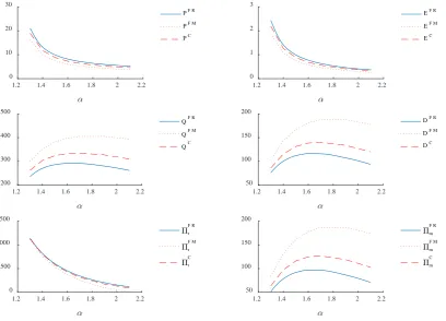
B. Sensitivity analysis with respect to demand elasticity

parameters

First, we consider how the optimal decisions and profits of the firms change with price elasticity of demand (α) in Models FR and FM. For comparison, we also consider Model C. The value of α ranges from 1.3 to 2.1 with an increment of 0.2. Tables A.3, A.4 and A.5 in the Appendix list the corresponding optimal decisions and profits for the three models respectively. Fig. 3 graphically illustrates the results in the tables.

1.2 1.4 1.6 1.8 2 2.2

0 10 20 30

PF R PF M PC

1.2 1.4 1.6 1.8 2 2.2

0 1 2 3

EF R EF M EC

1.2 1.4 1.6 1.8 2 2.2

200 300 400 500

QF R QF M QC

1.2 1.4 1.6 1.8 2 2.2

50 100 150 200

DF R DF M DC

1.2 1.4 1.6 1.8 2 2.2

0 500 1000 1500

r F R

r F M

r C

1.2 1.4 1.6 1.8 2 2.2

50 100 150 200

m F R

m F M

[image:6.595.71.513.155.750.2]

m C

Fig. 3. Sensitivity analysis with respect to price elasticity of demand

IAENG International Journal of Applied Mathematics, 48:3, IJAM_48_3_05

[image:6.595.96.505.467.761.2]

Fig. 3 further demonstrates the effect of introducing fairness into cooperative supply chain, which is discussed in the previous subsection. Furthermore, as α increases, the trends of the optimal decisions and profits are similar in the three models. In particular, as α increases, that is, as demand becomes more sensitive to the change of price, the supply chain will charge a lower retail price and expend a lower marketing effort, and the retailer will earn a lower profit. However, as α increases, the lot size and demand as well as the manufacturer’s profit increase first and then decrease. The initial increase of α may induce a

large reduction of retail price, which in turn leads to higher demand. As α continues to increase, the retail price decreases slowly, and the demand becomes decreasing.

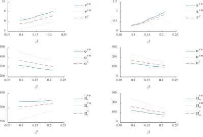
Next we consider how the optimal decisions and profits of the firms change with marketing expenditure elasticity of demand (β) in Models FR, FM and C. The value of β ranges from 0.09 to 0.21 with an increment of 0.03. Table A.6, A.7 and A.8 in the Appendix list the corresponding optimal decisions and profits for the three models respectively. Fig. 4 graphically displays the results in the tables.

0.05 0.1 0.15 0.2 0.25

4 6 8 10

PF R PF M PC

0.05 0.1 0.15 0.2 0.25

0 0.5 1 1.5

EF R EF M EC

0.05 0.1 0.15 0.2 0.25

200 300 400 500

QF R QF M QC

0.05 0.1 0.15 0.2 0.25

0 100 200 300

DF R DF M DC

0.05 0.1 0.15 0.2 0.25

200 300 400

r F R

r F M

r C

0.05 0.1 0.15 0.2 0.25

0 100 200 300

m F R

m F M

[image:7.595.96.496.214.483.2]

m C

Fig. 4. Sensitivity analysis with respect to marketing expenditure elasticity of demand

Fig. 4 also demonstrates the effect of introducing fairness into cooperative supply chain. In addition, the optimal decisions and profits change with β in a similar trend for the three models. Concretely speaking, as β increases, that is, as demand becomes more sensitive to the change of marketing effort, the retail price and marketing expenditure as well as the retailer’s profit increase, whereas the optimal lot size and demand as well as the manufacturer’s profit decrease.

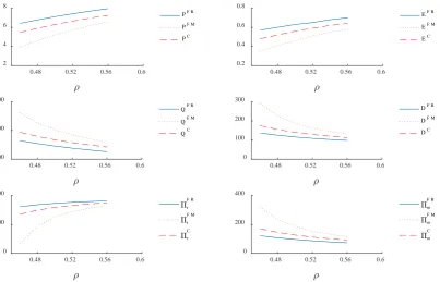
C. Sensitivity analysis with respect to bargaining power

parameter

We investigate the effects of bargaining power on the firms’ optimal decisions and profits. The value of bargaining power parameter

r

ranges from 0.46 to 0.56 with an increment of 0.02. Tables A.9, A.10 and A.11 in the Appendix provide the corresponding optimal decisions and profits for Models FR, FM and C respectively. Fig. 5 graphically shows the results in the tables.

Similar to Fig. 3 and Fig. 4, Fig. 5 illustrates the effect of incorporating fairness into cooperative supply chain. Furthermore, as

r

increases, the trends of the optimal decisions and profits are similar in the three models. In

particular, as the retailer’s bargaining power becomes larger, the retail price and marketing expenditure as well as the retailer’s profit increase, whereas the optimal lot size and demand as well as the manufacturer’s profit decrease. However, compared with the case with fairness-concerned retailer, the changes of the profits with respect to bargaining power are faster when the manufacturer is fairness-concerned.

Now we consider the impact of bargaining power on the total profit (see Fig. 6). When one firm cares about fairness, the total profit is decreasing with its bargaining power. Furthermore, when the retailer’s bargaining power is relatively small, incorporating fairness concern of the retailer into cooperative supply chain leads to a higher total profit, while incorporating fairness concern of the manufacturer leads to a lower total profit. When the retailer’s bargaining power is relatively large, the result is opposite. When the retailer’s bargaining power is intermediate, fairness concern of either firm leads to a lower total profit. Thus, when one firm has the advantage of bargaining power, the fairness concern of the other firm can improve the total profit.

IAENG International Journal of Applied Mathematics, 48:3, IJAM_48_3_05

However, the impact of bargaining power on the comprehensive utility is different from that on the total profit. As shown in Fig.7, no matter whether either firm is fairness-concerned, the comprehensive utility always increases with the retailer’s bargaining power. However, the existence of fairness concern reduces the comprehensive

utility. In addition, the comprehensive utility in the case with fairness-concerned manufacturer is lower than that in the case with fairness-concerned retailer, but the difference between them decreases as the retailer’s bargaining power becomes larger.

0.48 0.52 0.56 0.6 2

4 6 8

PF R PF M PC

0.48 0.52 0.56 0.6 0.2

0.4 0.6 0.8

EF R EF M EC

0.48 0.52 0.56 0.6 200

400 600

QF R QF M QC

0.48 0.52 0.56 0.6 0

100 200 300

DF R DF M DC

0.48 0.52 0.56 0.6 0

200 400

r F R

r F M

r C

0.48 0.52 0.56 0.6 0

200 400

m F R

m F M

[image:8.595.102.506.137.396.2]

m C

Fig. 5. Sensitivity analysis with respect to bargaining power parameter

0.46 0.48 0.5 0.52 0.54 0.56 0.58 380

390 400 410 420 430 440 450

[image:8.595.56.277.608.750.2]

F R F M C

Fig. 6. Sensitivity analysis of total profit with respect to bargaining power parameter

0.46 0.48 0.5 0.52 0.54 0.56 0.58 200

210 220 230 240

UF R

UF M UC

Fig. 7. Sensitivity analysis of comprehensive utility with respect to bargaining power parameter

VI. CONCLUSION

In this paper, we investigate the role of fairness in cooperative supply chain. While the existing literature focuses on the effect of fairness concern on decentralized supply chain, we innovatively introduce fairness concern into cooperative environment. Our analytical results show that the firms’ optimal decisions can be determined by using a one-dimensional search of only the lot size. Given the lot size, we find that cooperation can lead to a higher demand compared with decentralized supply chain, and fairness concern of the manufacturer in cooperative supply chain can further promote demand. We also show that when fairness concern of one firm is introduced into cooperative supply chain, an increase in its bargaining power can alleviate double marginalization effect. Our numerical results demonstrate the analytical results for cooperative supply chain. They also provide more insights on how the optimal decisions and profits change with fairness parameters, demand elasticity parameters and bargaining power parameter. Specifically, introducing fairness concern of one firm into cooperative supply chain can benefit that firm but hurt the other firm. As that firm becomes more fairness-concerned, he can earn more profit. Thus, fairness is an important factor to consider even when supply chain members cooperate.

There are several possible extensions to our study. First, we assume an unlimited production capacity. It would be interesting to incorporate capacity limitation when determining lot size. Second, as the first study on fairness in

IAENG International Journal of Applied Mathematics, 48:3, IJAM_48_3_05

cooperative supply chain environment, we consider the manufacturer’s and retailer’s fairness concerns separately. It would be worthwhile to explore the case where both firms are fairness-concerned. Finally, we assume that demand depends on retail price and marketing expenditure. It would be interesting to consider other formats of demand. Because these extensions require a very different mode of analysis, they will be left for future research.

APPENDIX

Tables of sensitivity analysis for Section Ⅴ.

Table A.1 Sensitivity analysis with respect to a in Model FR

a P E Q D Pr Pm

0 6.30 0.56 335.12 140.38 317.75 126.79 0.06 6.81 0.60 306.84 124.18 336.85 106.60 0.08 6.97 0.62 298.80 119.90 341.49 101.27 0.10 7.12 0.63 291.30 116.05 345.51 96.45 0.12 7.26 0.64 284.28 112.56 349.01 92.09 0.14 7.40 0.65 277.68 109.39 352.07 88.11

Table A.2 Sensitivity analysis with respect to b in Model FM

b P E Q D Pr Pm

0 6.30 0.56 335.12 140.38 317.75 126.79 0.06 5.69 0.50 372.37 164.38 285.68 156.84 0.08 5.46 0.48 387.75 175.14 270.08 170.40 0.10 5.22 0.46 405.16 187.92 250.71 186.56 0.12 4.96 0.44 425.11 203.31 226.29 206.12 0.14 4.68 0.41 448.27 222.18 194.91 230.26

Table A.3 Sensitivity analysis with respect to α in Model FR α _{P E} Q D Pr Pm

1.30 21.04 2.43 236.04 76.20 1141.15 51.40 1.50 9.91 0.99 286.18 112.01 604.59 91.76 1.70 7.12 0.63 291.30 116.05 345.51 96.45 1.90 5.89 0.46 280.32 107.47 202.99 86.50 2.10 5.22 0.37 261.88 93.79 119.92 70.91

Table A.4 Sensitivity analysis with respect to α in Model FM α _{P E} Q D Pr Pm

1.30 16.22 1.87 299.65 102.78 1107.50 83.68 1.50 7.37 0.74 382.15 167.18 532.17 160.86 1.70 5.22 0.46 405.16 187.92 250.71 186.56 1.90 4.27 0.34 405.46 188.19 96.97 186.90 2.10 3.76 0.27 394.05 177.75 10.73 173.92

Table A.5 Sensitivity analysis with respect to α in Model C α _{P E} Q D Pr Pm

1.30 18.95 2.19 262.19 85.93 1130.24 63.35 1.50 8.81 0.88 324.17 131.36 582.44 116.00 1.70 6.30 0.56 335.12 140.38 317.75 126.79 1.90 5.19 0.41 327.23 133.85 173.27 118.96 2.10 4.60 0.33 310.13 120.22 90.70 102.81

Table A.6 Sensitivity analysis with respect to β in Model FR β P E Q D Pr Pm

0.09 6.29 0.33 318.90 139.08 346.12 123.65 0.12 6.71 0.47 303.45 125.94 344.93 108.04 0.15 7.12 0.63 291.30 116.05 345.51 96.45 0.18 7.60 0.80 279.77 107.05 349.14 86.02 0.21 8.14 1.01 269.29 99.17 355.03 77.00

Table A.7 Sensitivity analysis with respect to β in Model FM β P E Q D Pr Pm

0.09 4.55 0.24 452.25 234.13 218.47 244.80 0.12 4.90 0.35 425.05 206.82 237.95 210.23 0.15 5.22 0.46 405.16 187.92 250.71 186.56 0.18 5.60 0.59 385.51 170.13 266.64 164.49 0.21 6.04 0.75 367.67 154.75 282.95 145.62

Table A.8 Sensitivity analysis with respect to β in Model C β P E Q D Pr Pm

0.09 5.54 0.29 369.65 170.80 309.39 163.79 0.12 5.90 0.42 351.25 154.22 312.55 143.51 0.15 6.30 0.56 335.12 140.38 317.75 126.79 0.18 6.74 0.71 320.69 128.56 324.78 112.66 0.21 7.23 0.89 307.58 118.26 333.55 100.49

Table A.9 Sensitivity analysis with respect to r in Model FR r _{P E Q D} P_r Pm

0.46 6.41 0.57 328.88 136.65 322.35 122.14 0.48 6.78 0.60 308.52 125.10 335.83 107.74 0.50 7.12 0.63 291.30 116.05 345.51 96.45 0.52 7.42 0.65 276.41 108.79 352.64 87.35 0.54 7.70 0.68 263.31 102.84 358.03 79.83 0.56 7.95 0.70 251.62 97.88 362.18 73.49

Table A.10 Sensitivity analysis with respect to r in Model FM r _{P E Q D}

r

P Pm

0.46 3.93 0.35 523.71 290.97 70.10 319.39 0.48 4.62 0.41 453.37 226.48 187.57 235.78 0.50 5.22 0.46 405.16 187.92 250.71 186.56 0.52 5.73 0.51 369.51 162.43 288.44 154.39 0.54 6.18 0.55 341.71 144.41 312.67 131.82 0.56 6.58 0.58 319.17 131.03 329.06 115.13

Table A.11 Sensitivity analysis with respect to r in Model C r _{P E Q D}

r

P Pm

0.46 5.46 0.48 387.75 175.14 270.08 170.40 0.48 5.90 0.52 358.66 155.20 298.43 145.32 0.50 6.30 0.56 335.12 140.38 317.75 126.79 0.52 6.65 0.59 315.51 128.96 331.46 112.55 0.54 6.97 0.62 298.80 119.90 341.49 101.27 0.56 7.26 0.64 284.28 112.56 349.01 92.09

REFERENCES

[1] S. Sang, "Supply Chain Coordination with Revenue Sharing Contract in Prospect Theory", IAENG International Journal of Applied Mathematics, vol. 47, no. 4, pp. 484-489, 2017.

[2] D. Corsten, N. Kumar, "Profits in the pie of the beholder", Harvard Business Review, vol. 81, no. 5, pp. 22-23, 2003.

[3] D. Corsten, N. Kumar, "Do suppliers benefit from collaborative relationships with large retailers? An empirical investigation of efficient consumer response adoption", Journal of Marketing, pp. 80-94, 2005.

[4] V. Manthou, M. Vlachopoulou, D. Folinas, "Virtual e-Chain (VeC) model for supply chain collaboration", International Journal of Production Economics, vol. 87, no. 3, pp. 241-250, 2004.

[5] C. Sheu, H. Rebecca Yen, B. Chae, "Determinants of supplier-retailer collaboration: evidence from an international study", International Journal of Operations & Production Management, vol. 26, no. 1, pp. 24-49, 2006.

[6] M. Esmaeili, M.-B. Aryanezhad, P. Zeephongsekul, "A game theory approach in seller–buyer supply chain", European Journal of Operational Research, vol. 195, no. 2, pp. 442-448, 2009.

[7] M. Rabin, "Incorporating fairness into game theory and economics",

The American Economic Review, pp. 1281-1302, 1993.

[8] E. Fehr, K. M. Schmidt, "A theory of fairness, competition, and cooperation", The Quarterly Journal of Economics, vol. 114, no. 3, pp. 817-868, 1999.

[9] G. E. Bolton, A. Ockenfels, "ERC: A theory of equity, reciprocity, and competition", American Economic Review, vol. 90, no. 1, pp. 166-193, 2000.

[10] T. H. Cui, J. S. Raju, Z. J. Zhang, "Fairness and channel coordination",

Management Science, vol. 53, no. 8, pp. 1303-1314, 2007.

[11] O. Caliskan-Demirag, Y. Chen, J. Li, "Channel coordination under fairness concerns and nonlinear demand", European Journal of Operational Research, vol. 207, no. 3, pp. 1321-1326, 2010.

[12] S. Du, C. Du, L. Liang, T. Liu, "Supply chain coordination considering fairness concerns", Jounal of Management Science in China, vol. 13, no. 11, pp. 41-48, 2010.

[13] L. Ma, "Supply chain Analysis with Fairness Preference Agent",

Operations Research and Management Science, vol. 20, no. 2, pp. 37-43, 2011.

IAENG International Journal of Applied Mathematics, 48:3, IJAM_48_3_05

[14] T.-H. Ho, X. Su, Y. Wu, "Distributional and Peer-Induced Fairness in Supply Chain Contract Design", Production and Operations Management, vol. 23, no. 2, pp. 161-175, 2014.

[15] S. Choi, P. R. Messinger, "The role of fairness in competitive supply chain relationships: An experimental study", European Journal of Operational Research, vol. 251, no. 3, pp. 798-813, 2016.

[16] H. Wang, M. Guo, J. Efstathiou, "A game-theoretical cooperative mechanism design for a two-echelon decentralized supply chain",

European Journal of Operational Research, vol. 157, no. 2, pp. 372-388, 2004.

[17] M. Nagarajan, G. Sošić, "Game-theoretic analysis of cooperation among supply chain agents: Review and extensions", European Journal of Operational Research, vol. 187, no. 3, pp. 719-745, 2008. [18] M. Leng, M. Parlar, "Allocation of Cost Savings in a Three-Level

Supply Chain with Demand Information Sharing: A Cooperative-Game Approach", Operations Research, vol. 57, no. 1, pp. 200-213, 2009.

[19] M. Cao, Q. Zhang, "Supply chain collaboration: Impact on collaborative advantage and firm performance", Journal of Operations Management, vol. 29, no. 3, pp. 163-180, 2011.

[20] K. Hidefumi, H. Toshimichi, S. Kiyoshi, "An Optimal Quantity Discount Policy for Deteriorating Items with a Single Wholesaler and Two Retailers", IAENG International Journal of Applied Mathematics, vol. 43, no. 2, pp. 81-86, 2013.

[21] W. J. Lee, D. Kim, "Optimal and heuristic decision strategies for integrated production and marketing planning", Decision Sciences, vol. 24, no. 6, pp. 1203-1214, 1993.

[22] X. Zhang, D. Yuan, "A Niche Ant Colony Algorithm for Parameter Identification of Space Fractional Order Diffusion Equation", IAENG International Journal of Applied Mathematics, vol. 47, no. 2, pp. 197-208, 2017.

[23] C. H. Loch, Y. Wu, "Social Preferences and Supply Chain Performance: An Experimental Study", Management Science, vol. 54, no. 11, pp. 1835-1849, 2008.

[24] N. Kumar, "The Power of Trust in Manufacturer-Retailer Relationships", Harvard Business Review, vol. 74, no. 6, pp. 15-19, 1996.

IAENG International Journal of Applied Mathematics, 48:3, IJAM_48_3_05