Shape Optimization Approach to the Bernoulli
Problem: A Lagrangian Formulation
Julius Fergy T. Rabago and Jerico B. Bacani
Abstract—The exterior Bernoulli free boundary problem is reformulated into a shape optimization setting by tracking the Dirichlet data. The shape derivative of the corresponding cost functional is established through a Lagrangian formulation coupled with the velocity method. A numerical example using the traction method orH1 gradient method is also provided.
Index Terms—Bernoulli free boundary problem, overdeter-mined boundary value problem, shape derivative, Lagrange method, minimax formulation.
I. INTRODUCTION
T
HE exterior Bernoulli free boundary problem (in two dimension) is formulated as follows: given a bounded and connected domain ω ⊂ R2 with a fixed boundary Γ :=∂ωand a constantλ <0, one needs to find a bounded connected domain B ⊂ U ⊂ R2 with a free boundary Σ := ∂B, containing the closure of ω, and an associated state function u: Ω→R, where Ω =B\ω¯, such that the overdetermined conditions are satisfied:
−∆u= 0 in Ω, u= 1 on Γ,
u= 0 on Σ,
∂νu=λ on Σ.
(1)
Here,ν is the outward unit normal vector to the free bound-aryΣ, and∂νu:=∂u/∂ν is the normal derivative ofu. The
Bernoulli problem appears in various physical systems that arise or can be seen in electrochemical machining, potential flow in fluid mechanics, tumor growth, etc. (cf. [1], [17], [18]).
In this paper, we are concerned with the reformulation of the ill-posed system (1) into the following shape optimization setting:
min
Σ J(Σ) = minΣ 1 2
∫
Σ
u2ds, (2)
whereu=u(Ω)satisfies the mixed boundary value problem
−∆u= 0 in Ω, u= 1 on Γ, ∂νu=λon Σ. (3)
Same as in [25], we want to characterize the shape derivative of the cost functionalJ overΣalong a perturbation fieldV.
This research was done under a project funded by the UP System Emerging Interdisciplinary Research Program (OVPAA-EIDR-C05-015). The publication was supported by UP System and UP Baguio.
J. F. T. Rabago was a research assistant of Prof. Bacani. He was a graduate of MS Mathematics program of the Department of Mathematics and Computer Science, College of Science, University of the Philip-pines Baguio, Governor Pack Road, Baguio City 2600, PhilipPhilip-pines. email: [email protected]
J. B. Bacani is an associate professor of mathematics and currently the chairman of the Department of Mathematics and Computer Science, College of Science, University of the Philippines Baguio, Governor Pack Road, Baguio City 2600, Philippines. e-mail: [email protected], [email protected].
We, however, establish the expression for the shape derivative ofJ using an approach independent from those exhibited in [25]. The novelty of this work is the alternative rigorous computation of the shape derivative of J derived from a Lagrangian formulation coupled with the velocity method. The shape derivativedJ(Σ;V) of J along the perturbation fieldVis obtained by going to the limit of[J(Σt)−J(Σ)]/t,
where Σt is the result of perturbing the free boundary Σ
through a non-autonomous perturbation fieldV. Meanwhile, the idea behind the Lagrange method is to rewrite the cost function under consideration as the min-max of an appropriate Lagrangian; that is, a utility function plus the equality constraints. As a consequence, the differentiability of the cost functional is transferred to the differentiability of the Lagrangian with respect to a particular parameter, which is, in our case, the variable t. In this regard, one needs a theorem to differentiate a minimax or the saddle point of a Lagrangian with respect to a parameter. Fortunately, a very powerful tool to fulfil the task has already been established in [13]. Its application to shape sensitivity analysis, however, is not completely straightforward because it leads to the time dependence of the underlying function spaces appearing in the minimax formulation [15]. Nevertheless, two techniques can be employed to get around this difficulty: the function space parameterization and the function space embedding techniques (cf. [14, Section 10.2.2, p. 522–523 and Section 10.6]). It is worth noting that Lagrange methods have the advantage of providing the shape derivative of cost func-tionals without the need to compute the shape and material derivative of the states. Some recent studies examining the shape derivatives of cost functionals through Lagrangian methods were delivered in [9], [19], [20], [26], [28], and [29].
The rest of the paper is organized as follows. In the next section, we give the essentials of our present investigation. The Lagrangian formulation of the problem is formally presented in Section III. The minimax formulation is coupled with the function space parametrization and function space embedding technique so that a theorem on the differentia-bility of a saddle point (i.e., a minimax) of a Lagrangian functional with respect to a parameter can be applied. After computing the shape gradient, we give a concrete example in Section IV and numerically solve the problem using the traction method or H1 gradient method. In Section V, we give a concluding remark regarding the present study.
II. PRELIMINARIES
In this section, we give the requisites of our study. First, we give a brief discussion about the velocity method.
Let V be an element of Ek = C([0, tV);Dk(R2,R2)),
for some integer k ≥ 2 and a small real number tV > 0,
IAENG International Journal of Applied Mathematics, 47:4, IJAM_47_4_07
whereDk(R2,R2)denotes the space ofk-times continuously differentiable functions with compact support contained in R2. The field V(t)(x) = V(t, x), x ∈ R2, is an element of Dk(R2,R2) which may depend on t ≥ 0. It generates the transformations Tt(V)(X) :=Tt(X) =x(t;X), t≥0,
X ∈R2, through the differential equation
d
dtx(t;X) =V(t, x(t;X)), x(0;X) =X, (4)
with the initial value X given. We denote the “transformed domain” Tt(V)(Ω) at t ≥ 0 by Ωt(V), or simply Ωt =:
Tt(Ω). In this work, we shall consider annular domains Ωt
with boundary∂Ωt, which is the union of two disjoint sets Γt and Σt, referred to as the fixed and free boundaries,
respectively. The evolutions of the domain Ω are obtained using non-autonomous velocity fields
V(t)(x)∈ V:={V(t, x)∈C1,1([0, tV]×U ,R2) :V|Γ∪∂U= 0}. (5) For t ∈ [0, tV], Tt is invertible and Tt, T−1
t ∈ D
1(R2,R2)
(cf. [7, Lemma 11], [8, Lemma 2.4]). In addition, the Jacobian It is strictly positive, i.e., It = |detDTt(X)| > 0, where DTt(X)is the Jacobian matrix of the transformationTt=Tt(V)
associated with the velocity fieldV. In this paper, the expressions
(DTt)−1 and (DTt)−T refer to the inverse and transpose of the the Jacobian matrix, respectively. Also, we use the notation At =It(DT−1)(DTt)−T, andwt =It|(DTt)−Tν|, whereDTt is the Jacobian matrix ofTtwith respect to the boundary∂Ω.
For the rest of this section we state the essentials of our analysis. Proposition 1: For a function φ∈Wloc1,1(R2)
and V∈ V, we have the following formulas
(i) ∇(φ◦Tt) = (DTt)T(∇φ)◦Tt, (ii) d
dt(φ◦Tt) = (∇φ·V(t))◦Tt, (iii) d
dt(φ◦T
−1
t ) =−(∇φ·V(t))◦T−
1
t ,
(iv) d
dtIt= divV(t)◦TtIt,
(v) w′t|t=0= limt↘0 1t(wt−w0) = divΣV(0),
wheredivΣdenotes the surface divergence and is defined by
divΣV(0) = div(V(0))−DV(0)ν·ν.
The above results can be found in [14], [31], and are given as properties of the transformationTtin [7], [23], [25].
Lemma 1 ( [31]): We have the following domain and boundary transformations:
(i) Ifφt∈L1(Ω
t)then,φt◦Tt∈L1(Ω)and ∫
Ωt
φtdxt=
∫
Ω
φt◦TtItdx.
(ii) Ifφt∈L1(Σt)then,φt◦Tt∈L1(Σ)and ∫
Σt
φtdst=
∫
Σt
φt◦Ttwtds.
We are now ready to examine the shape derivative ofJthrough a Lagrangian formulation in the next section.
III. MAINRESULTS
Minimax Formulation
In this section we established the shape derivative ofJ through a Lagrangian formulation. To begin with, we recall the variational form of system (3):
Findu∈H1(Ω)such that ∫
Ω
∇u· ∇φ− ∫
Σ
λφ= 0, ∀φ∈HΓ1,0(Ω); u= 1 on Γ. (6)
Since we have an essential boundary conditionu= 1onΓ, which is tied with the definition of the function spaceHΓ1,0(Ω), we introduce
the Lagrangian multiplierµ∈H1/2(Γ)and express the variational
form (6) of (3) as follows ∫
Ω
∇u· ∇φdx− ∫
Σ
λφds+
∫
Γ
(u−1)µds= 0, ∀φ∈HΓ1,0(Ω).
To express this equation in terms of just one variable, we take µ=∂νφto obtain
∫
Ω
∇u·∇φdx− ∫
Σ
λφds+
∫
Γ
(u−1)∂νφds= 0,∀φ∈HΓ1,0(Ω).
Now, we introduce the functional
G(Σ, φ, ψ) =F(Σ, φ)+L(Σ, φ;ψ),∀φ∈H1(Ω),∀ψ∈HΓ1,0(Ω),
(7)
where F(Ω, φ) := J(φ,Σ) = J(Σ), and L(Σ, φ;ψ) is the Lagrangian functional given by
L(Σ, φ;ψ) =
∫
Ω
∇φ· ∇ψdx− ∫
Σ
λψds+
∫
Γ
(φ−1)∂νψds.
Given this construction ofG, one can easily check that
J(Σ) = min
φ∈H1(Ω)ψ∈maxH1 Γ,0(Ω)
G(Σ, φ, ψ),
since
max
ψ∈H1 Γ,0(Ω)
G(Σ, φ, ψ) =
{
F(Ω, φ), ifφ=u,
+∞, otherwise.
It is easily shown that the functionalGis convex continuous with respect toφand concave continuous with respect toψ. Therefore, according to Ekeland and Temam [16], the functionalGhas a saddle point(u, p)if and only if(u, p)solves the following system
L(Σ, u;φ) = 0, ∀φ∈HΓ1,0(Ω),
dF(Σ, u;φ) +dL(Σ, u, p;φ) = 0, ∀φ∈HΓ1,0(Ω),
or equivalently,
−∆u= 0 in Ω, u= 1 on Γ, ∂νu=λon Σ; (8)
−∆p= 0 in Ω, p= 0 on Γ, ∂νp=−uon Σ. (9) Similarly, the previous analysis holds in the transformed domainΩt under the action of the velocity fieldVfort≥0. Thus, we have
J(Σt) = min φ∈H1(Ωt)
max
ψ∈H1 Γ,0(Ωt)
G(Σt, φ, ψ),
whose unique saddle point(ut, pt)is completely characterized by the system
L(Σt, ut;φ) = 0, ∀φ∈HΓ1,0(Ωt), dF(Σt, ut;φ) +dL(Σ, ut, pt;φ) = 0, ∀φ∈HΓ1,0(Ωt),
or equivalently, ∫
Ωt
∇ut· ∇φdxt− ∫
Σt
λφdst+
∫
Γ
(ut−1)∂νφds= 0,
∀φ∈HΓ1,0(Ωt); (10)
∫
Ωt
∇pt· ∇φdxt+
∫
Σt
utφdst= 0, ∀φ∈HΓ1,0(Ωt). (11)
Our next objective is to find the limit
dj(0) = lim
t↘0
j(t)−j(0)
t ,
where
j(t) :=J(Σt) = min φ∈H1(Ωt)
max
ψ∈H1 Γ,0(Ωt)
G(Σt, φ, ψ).
Hereon, we need a theorem that would give the derivative of the minimax with respect to a parametert≥0att= 0. Unfortunately, the Sobolev spacesH1(Ωt)andHΓ1,0(Ωt)depend on the parameter t. To overcome this difficulty and obtain an infimum with respect to
IAENG International Journal of Applied Mathematics, 47:4, IJAM_47_4_07
a function space that is independent oft, we can use two techniques [14], namely:
• Function space parametrization technique; and
• Function space embedding technique.
We will first use the idea of function space parametrization technique below, followed by the application of function space embedding technique afterwards.
Function Space Parametrization Technique
This section is devoted to the application of function space parametrization technique to the problem. It consists of transporting the quantities defined in the variable domain Ωt back into the reference domain Ω. Once the technique is employed, the usual methods in differential calculus can now be applied since the functionals involved are now defined in a fixed domainΩ. The idea is to parametrize the functions inH1(Ω
t)by elements ofH1(Ω) through the transformation φ 7→ φ◦Tt−1 : H1(Ω) →H1(Ωt). Since Tt and Tt−1 are diffeomorphisms (cf. [7, Thm. 7]), it transforms the domain Ω into Ωt and changes the boundary Σ to the boundary Σt of Ωt. In particular, since V ∈ C1,1, we have φ◦Tt−1 ∈ H
1
(Ωt) for all φ ∈ H1(Ω), and conversely, ψ◦Tt ∈ H1(Ω) for all ψ ∈ H1(Ωt). Also, we introduce the parametrization HΓ1,0(Ωt) = {φ◦Tt−1 : φ ∈ H
1
Γ,0(Ω)}. These
parametrizations do not affect the value of the minimumJ(Σt)but changes the Lagrangian functionalG:
J(Σt) = min
φ∈H1(Ω)ψ∈maxH1 Γ,0(Ω)
G(Σt, φ◦Tt−1, ψ◦T−
1
t ).
Given this formulation, we define a new Lagrangian
˜
G(t, φ, ψ) :=G(Σt, φ◦Tt−1, ψ◦T−
1
t ),
that is,
˜
G(t, φ, ψ) =1 2
∫
Σt
(φ◦Tt−1)
2
dst
+
∫
Ωt
∇(φ◦Tt−1)· ∇(ψ◦T−
1
t ) dxt
− ∫
Σt
λ(ψ◦Tt−1) dst
+
∫
Γ
(φ◦Tt−1−1)∂ν(ψ◦T−
1
t ) ds, (12)
for allφ∈H1(Ω)andψ∈HΓ1,0(Ω). The saddle point of this new
Lagrangian is completely characterized by the following variational systems:
State equations. Findut∈H1(Ω)such that
∫
Ωt
∇(ut◦Tt−1)· ∇(φ◦T−
1
t ) dxt− ∫
Σt
λ(φ◦Tt−1) dst
+
∫
Γ
(ut◦Tt−1−1)∂ν(φ◦T−
1
t ) ds= 0, ∀φ∈H
1 Γ,0(Ω).
(13)
Adjoint state equations. Findpt∈HΓ1,0(Ω)such that
∫
Ωt
∇(pt◦Tt−1)· ∇(ψ◦T−
1
t ) dxt
+
∫
Σt
(ut◦Tt−1)(ψ◦T−
1
t ) dst= 0, ∀ψ∈H
1 Γ,0(Ω).
(14)
Remark 1: Comparing these expressions with the characteriza-tion of the minimizing element(ut, pt)ofG(Σt,·,·)onH1(Ωt)× HΓ1,0(Ωt) which satisfies equations (10) and (11), we see that ut=ut◦Tt−1,u
t
=ut◦Tt,pt=pt◦Tt−1 andp t
=pt◦Tt. So,
(ut, pt)is actually the solution(ut, pt)of equations (10) and (11) in Ωt transported back onto the fixed domainΩby the change of variables induced by the transformationTt.
Using the transformationTt and Proposition 1(i), we can rewrite the Lagrangian (12) onΩas
˜
G(t, φ, ψ) =1 2
∫
Σ
wtφ2ds+
∫
Ω
At∇φ· ∇ψdx
− ∫
Σ
wtλψds+
∫
Γ
wt(φ−1)∂νψds. (15)
Furthermore, in view of Lemma 1, we find that the saddle point
(ut, pt)
of the above Lagrangian is, in fact, the solution of the following variational systems:
State equations. Findut∈H1(Ω)such that ∫
Ω
At∇ut· ∇φdx− ∫
Σ
wtλφds
+
∫
Γ
wt(ut−1)∂νφds= 0,∀φ∈HΓ1,0(Ω). (16)
Adjoint state equations. Findpt∈HΓ1,0(Ω)such that
∫
Ω
At∇pt· ∇φdx+
∫
Σ
wtutφds= 0, ∀φ∈HΓ1,0(Ω). (17)
Hereafter, a theorem concerning the differentiability of a minimax will come into play. In particular, we will apply Theorem 2 (see Appendix) due to [13] in order to get the first-order shape derivative ofJ. To do this, we need to verify the four assumptions (H1)–(H4) of the theorem.
Verification of Condition (H1). First, assume that V ∈ V. Choose a sufficiently small number τ > 0 such that there exist two constantsα1, α2 (0< α1 < α2),α1 ≤It(=|It|)≤α2, for
allt∈[0, τ](cf. [7, Lem. 6]). So, we can find a numberβ >0such thatAt ≥βI2 for all t∈[0, τ], whereI2 is the two-dimensional
identity matrix (cf. [7, Lem. 11]). The existence and uniqueness of solutionut of (13) is now easily verified as shown in [7, Sec. 4.2]. Meanwhile, the existence and uniqueness of solutionptof (14) can also be shown by following a similar reasoning delivered in [7, Sec. 4.2], and by taking the test functionφ=pt in (17). Hence,
∀t∈[0, τ] : X(t) ={ut} ̸=∅, Y(t) ={pt} ̸=∅.
Thus, (H1) is satisfied.
Verification of Condition (H2). The partial derivative of
˜
G(t, φ, ψ)with respect to the parametertis characterized by
∂tG˜(t, φ, pt) =1 2
∫
Σ
w′tφ
2
ds+
∫
Ω
A′t∇φ· ∇ψdx− ∫
Σ
w′tλψds.
SinceV∈D1(R2,R2), thent7→DTt is continuous in[0, τ](cf.
[7, Lemma 11]). Hence,∂tG˜(t, φ, φ) is well-defined and it exists everywhere on[0, τ], for allφ∈H1(Ω)andψ∈HΓ1,0(Ω). Thus,
assumption (H2) is satisfied.
Verification of Conditions (H3) and (H4). We first show that for any sequence{tn} ⊂[0, τ],such thattn→0, there exists a sub-sequence of{utn, ptn}(which is still denoted by{utn, ptn}) such that(utn, ptn)⇀(u0
, p0) = (u, p)weakly inH1(Ω)×HΓ1,0(Ω),
where(u, p)is the solution of systems (8) and (9). To do this, we need to show that(ut, pt)
is bounded inH1(Ω)×H1
Γ,0(Ω). In view
of the discussion delivered in [7], one easily finds thatutis bounded inH1(Ω). Also, following a similar line of arguments laid out in [7, Section 4.2], we find thatptis bounded inHΓ1,0(Ω). Hence, the
pair(ut, pt) is bounded in H1(Ω)×HΓ1,0(Ω), and so, there is a
subsequence{utn, ptn}and a pair(z, q)inH1(Ω)×H1
Γ,0(Ω)such
that (utn, ptn) ⇀(z, q) weakly inH1(Ω)×H1
Γ,0(Ω). The pair
(z, q)can be characterized by passing to the limit in the variational equations
∫
Ω
Atn∇u
tn· ∇φdx− ∫
Σ
wtnλφds
+
∫
Γ
wtn(u
tn−1)∂νφds= 0, ∀φ∈H1 Γ,0(Ω);
∫
Ω
Atn∇p
tn· ∇φdx+ ∫
Σ
wtnu
tnφds= 0, ∀φ∈H1 Γ,0(Ω).
IAENG International Journal of Applied Mathematics, 47:4, IJAM_47_4_07
By passing to the limit,(z, q)is characterized by ∫
Ω
∇z· ∇φdx− ∫
Σ
λφds+
∫
Γ
(z−1)∂νφds= 0,
∀φ∈HΓ1,0(Ω);
∫
Ω
∇q· ∇φdx+
∫
Σ
zφds= 0, ∀φ∈HΓ1,0(Ω).
By uniqueness (z, q) = (u, p), where (u, p) is the solution to systems (13) and (14) at t = 0; that is, the pair (u, p) satisfies the system
∫
Ω
∇u· ∇φdx− ∫
Σ
λφds+
∫
Γ
(u−1)∂νφds= 0,
∀φ∈HΓ1,0(Ω);
∫
Ω
∇p· ∇φdx+
∫
Σ
uφds= 0, ∀φ∈HΓ1,0(Ω).
Furthermore, we can deduce the H1(Ω)×L2(Ω)-strong con-vergence: (utn, ptn) → (u, p). Hence, (H3)(i) and (H4)(i) are satisfied for theH2(Ω)×H1(Ω)-strong topology by the classical regularity theorem (cf. [21]). Finally, assumptions (H3)(ii) and (H4)(ii) are readily satisfied in view of the strong continuity of
(t, φ, ψ)7→∂tG˜(t, φ, ψ).
We have just shown that all of the four assumptions in Theorem 2 are satisfied, and so, we have the derivative
dJ(Σ;V) =∂tG˜(t, u, p)|t=0=
1 2
∫
Σ
w′0u 2
ds
+
∫
Ω
A′0∇u· ∇pdx−
∫
Σ
w′0λpds. (18)
HereA′0 =A=: divVI2−(DV+ (DV)T)and w0′ = divΣV.
This expression for the shape derivative of J can be written in terms of the boundary integral. To do this, we recall the following result whose proof can be found in [1] (see also [7, Lem. 32] for an alternative proof).
Lemma 2: Letφ, ψ∈H2(Ω)
, whereΩis aC1,1
-domain having the boundary ∂Ω = Γ∪Σ (Γ∩Σ =∅), andV be a vector field belonging toV. Then,
∫
Ω
A∇φ· ∇ψdx=
∫
Ω
∆φ(V· ∇ψ) dx
+
∫
Ω
∆ψ(V· ∇φ) dx+
∫
Σ
(∇φ· ∇ψ)V·νds
− ∫
Σ
∂νφ(V· ∇ψ) ds− ∫
Σ
∂νψ(V· ∇φ) ds.
Takingφandψasuandpin the previous lemma, and noting that they satisfy equations (8) and (9), respectively, we get
∫
Ω
A∇φ· ∇ψdx=
∫
Σ
(∇u· ∇p)V·νds
− ∫
Σ
∂νu(V· ∇p) ds− ∫
Σ
∂νp(V· ∇u) ds
=
∫
Σ
(∇u· ∇p)V·νds− ∫
Σ
λ(V· ∇p) ds
+
∫
Σ
u(V· ∇u) ds.
However,∇(u2) = 2u∇u, so
∫
Ω
A∇φ· ∇ψdx=
∫
Σ
(∇u· ∇p)V·νds
− ∫
Σ
λ(V· ∇p) ds+1 2
∫
Σ
(V· ∇u2) ds.
Therefore, the computed shape derivative (18) is equivalent to
dJ(Σ;V)
=
∫
Σ
[
V· ∇
( 1 2u 2 +λp ) + ( 1 2u 2 +λp )
divΣV
]
ds
+
∫
Σ
(∇u· ∇p)V·νds. (19)
We further characterize the derivativedJ(Σ;V). First, we note that the mapV ∋ V 7→dJ(Σ;V) is linear and continuous (cf. [7]), and soJ(Σ)is indeed shape differentiable. Then, according to Hadamard-Zol´esio structure theorem (cf. [14]), there is a scalar distribution g ∈ D1(Σ)′ such that dJ(Σ;V) = ∫ΣgΣV·νds.
If we assume that the boundary ofΩis a C1,1
, then we see that
(u, p) ∈ H2(Ω)×(H2(Ω)∩H1
0(Ω)) (cf. [7, Thm. 29]). This
regularity of the pair(u, p)implies that we can use the Hadamard’s domain and boundary differentiation formulas [14]:
d dt
{∫
Ωt
F(t, x) dxt} t=0
=
∫
Ω
∂tF(0, x) dx
+
∫
∂Ω
F(0, s)V·νds; (20)
d dt
{∫
∂Ωt
F(t, x) dst} t=0
=
∫
∂Ω
∂tF(0, s) ds
+
∫
∂Ω
(∂νF+κF(0, s))V·νds,
(21)
where F : [0, τ]×Rd → R is a sufficiently smooth functional. Thus, we can compute the partial derivative∂tG˜(t, u, p) from the expression (12) using the above formulas. That is, we have
∂tG˜(0, u, p) = d
dt{I1(t) +I2(t) +I3(t) +I4(t)}
t=0
,
where
I1(t) =
1 2
∫
Σt
(u◦Tt−1)
2
dst;
I2(t) =
∫
Ωt
∇(u◦Tt−1)· ∇(p◦T−
1
t ) dxt;
I3(t) =
∫
Γt
(u◦Tt−1−1)∂ν(p◦T−
1
t ) dst;
I4(t) =−
∫
Σt
λ(p◦Tt−1) dst.
Taking into account Proposition 1(iii), the expressions for I′1(0),
I′2(0),I′3(0)andI′4(0)are easily computed as follows. For the first
integral, we have
d dtI1(t)
t=0 = ∫ Σ ∂t [ 1 2(u◦T
−1 t ) 2] t=0 ds + ∫ Σ [ ∂ν ( 1 2u 2 )
+κ1
2u
2
]
V·νds
=−
∫
Σ
u(∇u·V) ds+1 2
∫
Σ
(
∂νu2+κu2)V·νds.
Meanwhile,
d dtI2(t)
t=0 = ∫ Ω
∂t{∇(u◦Tt−1)· ∇(p◦T−
1
t )}t=0 dx
+
∫
∂Ω
(∇u· ∇p)V·νds
=
∫
Ω
∂t{∇(u◦Tt−1)}t=0∇pdx
+
∫
Ω
∂t{∇(p◦Tt−1)}t=0∇udx
+
∫
∂Ω
(∇u· ∇p)V·νds
=
∫
Ω
∇(−∇u·V)∇pdx
+
∫
Ω
∇(−∇p·V)∇udx+
∫
∂Ω
(∇u· ∇p)V·νds.
IAENG International Journal of Applied Mathematics, 47:4, IJAM_47_4_07
We know by definition that the perturbation fieldVvanishes at the fixed boundaryΓ, i.e.,V|Γ = 0. Hence, by Green’s first identity,
we obtain the following simplification forI′2(0):
d dtI2(t)
t=0
=
∫
Ω
∆p(∇u·V) dx− ∫
Σ
∂νp(∇u·V) ds
+
∫
Ω
∆u(∇p·V) dx− ∫
Σ
∂νu(∇p·V) ds
+
∫
∂Σ
(∇u· ∇p)V·νds.
Note thatuandpare solutions of systems (8) and (9), respectively. So,
d dtI2(t)
t=0
=−
∫
Σ
p(∇u·V) ds− ∫
Σ
λ∇p·Vds
+
∫
Σ
(∇u· ∇p)V·νds.
For the third integral, we have
d dtI3(t)
t=0
=
∫
Γ
∂t[(u◦Tt−1−1)∂ν(p◦T−
1
t )]t=0ds
− ∫
Γ
[∂ν((u−1)∂νp) +κλp]V·νds
=−
∫
Γ
[∇u·V∂νp+u∇(∂νp)·V] ds
− ∫
Γ
[∂ν((u−1)∂νp) +κλp]V·νds.
ButVvanishes atΓ, so,I′3(0) = 0.
Remark 2: The above computation of the derivative I′2(0)
pro-vides an alternative proof of Lemma 2 which was proven in [7] and [25] in different ways.
Finally, for the fourth integral, we have
d dtI4(t)
t=0
= d
dt {
− ∫
Σt
λ(p◦Tt−1) dst }
t=0
=−
∫
Σ
∂t[λ(p◦Tt−1)]t=0ds
− ∫
Σ
[∂ν(λp) +κλp]V·νds
=
∫
Σ
λ∇p·Vds− ∫
Σ
(λ∂νp+κλp)V·νds.
Adding all these terms yields the desired expression fordJ(Σ;V), that is,
dJ(Σ;V)
=
∫
Σ
[ ∂ ∂ν
(
1 2u
2−
λp )
+
(
1 2u
2−
λp )
κ+∇u· ∇p ]
V·νds.
The above result can be obtained directly from (19). To see this, one simply employs the following result referred to as the tangential Green’s formula (cf. [23, Lemma 3.3], [8, Lemma 2.15, Eq. 19]).
Lemma 3 (Tangential Green’s formula): Let U be a bounded domain of classC1,1 andΩ⊂U with boundaryΓ. Also consider
V∈C1,1([0, tV]×U ,R2)andf∈W2,1(U)
∫
Γ
(fdivΓV +∇Γf·V) ds=
∫
Γ
κfV·νds, (22)
where κ is the curvature ofΓ and the tangential gradient ∇Γ is
given by
∇Γf=∇f|Γ−(∂νf)ν.
By using (19) and by takingf= 1 2u
2−λp
in equation (22), we get the same expression for the shape derivativedJ(Σ;V). In summary, we have proven the following result differently from [25].
Theorem 1: LetΩ⊂R2 be aC1,1-bounded domain and con-sider the shape optimization problem (2) where the state function uis the solution of the mixed-boundary value problem (3). Then,
the shape derivative ofJ atΣin the direction of the perturbation fieldV∈ V, whereVis defined by (5), is given by
dJ(Σ;V)
=
∫
Σ
[ ∇
(
1 2u
2−
λp )
·V+
(
1 2u
2−
λp )
divΣV
]
ds
+
∫
Σ
[(∇u· ∇p)V·ν] ds.
Further, ifΣhasC2-regularity (or∂ΩisC1,1), then
dJ(Σ;V)
=
∫
Σ
[ ∂ ∂ν
(
1 2u
2−
λp )
+
(
1 2u
2−
λp )
κ ]
V·νds
+
∫
Σ
[∇u· ∇p]V·νds. (23)
Here, the adjoint statep∈HΓ1,0(Ω)satisfies the variational equation
∫
Ω
∇p· ∇ψdx+
∫
Σ
uψds= 0,
for allψ∈H1 Γ,0(Ω).
A. Function Space Embedding Technique
This section is devoted to the function space embedding tech-nique. It means that the state and adjoint states are defined on a large enough domainD called ahold-all[14] which contains all the transformations{Ωt : 0≤t≤τ} of the reference domainΩ for some small enough numberτ >0.
LetD=R2. Then we differentiate with respect totthe minimax
J(Σt) = min
Φ∈H1(R2)Ψ∈Hmax1 Γ,0(R2)
G(Σt,Φ,Ψ),
where the new Lagrangian functionalG(Σt,Φ,Ψ)is given by
G(t,Φ,Ψ) =1 2
∫
Σt
Φ2dst+
∫
Ωt
∇Φ· ∇Ψ dxt
− ∫
Σt
λΨ dst+
∫
Γ
(Φ−1)∂νΨ. (24)
For sufficiently smooth domain Ωt (in our case ∂Ωt is C1,1), the unique solution (ut, pt) of systems (16) and (17) belongs to H2(Ωt)×(H2(Ωt)∩HΓ1,0(Ωt))instead ofH1(Ωt)×HΓ1,0(Ωt). Therefore, the set X×Y ⊂ H2(R2)×H2(R2) and the set of saddle points S(t) = X(t)×Y(t), which is not a singleton set anymore, are given by
X(t) ={Φ∈H2(R2) : Φ|Ωt =ut}; Y(t) ={Ψ∈H2(R2) : Ψ|Ωt =pt},
where(ut, pt)is the unique solution in H2(Ω
t)×H2(Ωt) to the saddle point equations (16) and (17).
We now verify the four assumptions of Theorem 2.
Verification of Condition (H1). Construct a linear and continu-ous extension Π : H2(Ω) → H2(R2)
and define an extension
Πt:H2(Ωt)→H2(R2),Π(ϕ) = [Π(ϕ◦Tt)]◦Tt−1. We see that we can define the extensionsΦt= ΠtutandΨt= Πtpt ofutand pt, respectively. So,Φt ∈X(t) and Ψt ∈Y(t). These show the existence of a saddle point, i.e.,S(t)̸=∅. Thus, (H1) is satisfied.
Verification of Condition (H2). To check (H2), we compute the partial derivative of the expression (24) using Hadamard’s formulas (20) and (21):
∂tG(t,Φ,Ψ) =
∫
Σt (
∂ ∂ν
(
1 2Φ
2
)
+1 2Φ
2
κ )
Vt·νtdst
+
∫
Ωt
(∇Φ· ∇Ψ)Vt·νtdxt
− ∫
Σt (
∂(λΨ)
∂ν +λΨκ )
Vt·νtdst, (25)
IAENG International Journal of Applied Mathematics, 47:4, IJAM_47_4_07
whereνtdenotes the outward unit normal to the boundaryΣt. Since
V∈D1(R2,R2), the expression∂tG(t,Φ,Ψ)exists everywhere in
[0, τ]for all(Φ,Ψ)∈H1(R2)×H1(R2). Hence (H2) is satisfied.
Verification of Conditions (H3) and (H4). For C1,1-domain Ω
and vector fieldsV∈D1(R2,R2), we have shown in Section III that(ut, pt)converges to(ut, pt)in theH2×H1-strong topology as tgoes to zero. Hence, Φt →Φ = Πut and Ψt →Ψ = Πpt strongly inH2(R2)
by using the following lemma.
Lemma 4 ( [14]): Given any integer m ≥ 1, a velocity field
V ∈Dm(Rd,Rd), and a function Π∈Hm(Rd), if ut →u0 in
Hm(Ω)-strong, then Φ
t → Φ0 in Hm(Ω)-strong, where Φt :=
(Πut)◦T−1
t . One can also show that the above result also holds for the weak topology ofHm(Rd)
.
Furthermore, assumptions (H3)(i) and (H4)(i) are satisfied for theH2×H2-strong topology.
Now let us check (H3)(ii) and (H4)(ii). Since (Φ,Ψ) ∈
H2(R2)×H2(R2), we can use Stoke’s formula to rewrite (25) as
∂tG(t,Φ,Ψ)
=
∫
Ωt
div
{[( ∂ ∂ν
(
1 2Φ
2
)
+1 2Φ
2
κ )
+ (∇Φ· ∇Ψ)
]
Vt
}
dxt
− ∫
Ωt
div
{[( ∂(λΨ)
∂ν +λΨκ )]
Vt
}
dxt
=:
∫
Ωt
div(FVt)dxt.
Here we have used the fact that∂Ωt= Γ∪Σtand thatVvanishes on the boundary Γ. Evidently, the map (Φ,Ψ) 7→ F(Φ,Ψ) is bilinear and continuous. Similarly, sinceV∈D1(R2,R2), the map
(t, F)7→
∫
Ω
(divFVt)◦TtItdx
from [0, τ]×X ×Y to Ris continuous. Therefore, (H3)(ii) and (H4)(ii) are verified. This completes the verification of the four assumptions of Theorem 2.
Consequently, we obtain
dJ(Σ;V) = min
Φ∈X(0)Ψmax∈Y(0)∂tG(t,Φ,Ψ)|t=0. (26)
Furthermore, we note that the expression (25) can be expressed in terms of a boundary integral onΣ(as shown in the previous section) which will not depend on(Φ,Ψ)outside ofΩt. So, the inf and the sup in (26) can be dropped, giving us the same expression as in (23). This ends the computation.
IV. NUMERICALEXAMPLE
The existence of optimal solution of the shape optimization problem (2)-(3) has already been studied in [10], and so we just carry out here a numerical realization of the optimization problem. To numerically solve the shape optimization problem, we employ an iterative algorithm based on theH1gradient method. This method was introduced in [3] and was then called the traction method (see also [4]). It was later on referred to as the H1
gradient method in [5], and was compared with other techniques was described in [6]. The basic idea of the gradient method in a Hilbert space was presented in [27]. For more details of this method, we refer the readers to the aforementioned papers.
The optimization algorithm using theH1 gradient method can be summarized as follows:
1) Define an initial domainΩ0 with boundary∂Ω0= Γ∪Σ0,
Γ∩Σ0=∅, and generate a finite element mesh on the given
domain.
2) Solve the state equation (10) and the adjoint state equation (11) on the current domainΩ0.
3) Compute the descent directionVk by traction method, i.e., by solving the following PDE system
−∆V+V= 0 in Ω, V= 0 on Γ, ∂V
∂ν =−Gνon Σ, where Gdenotes the kernel of the shape gradient given in (23) with the domainΩ = Ωk.
4) Modify the current domain by the perturbation fieldVk to obtain a new domain. That is, defineΩk+1:={x+tkVk(x) : x ∈ Ωk}, for sufficiently small tk > 0, together with the nodal points of the mesh.
5) Repeat step 2-4 until the domainΩk converges.
For a concrete example of the problem, we consider the shape optimization reformulation (2)-(3) of (1) withλ=−1. That is, we consider the following optimization problem:
min
Σ J(Σ) = minΣ
1 2
∫
Σ
u2ds
where the state variableusatisfies
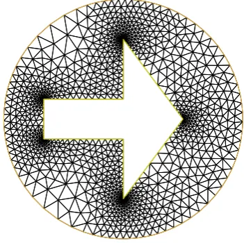
[image:6.595.52.289.245.329.2]−∆u= 0 in Ω, u= 1 on Γ, ∂νu=−1 on Σ. (27) We consider a fixed boundaryΓconstructed in an arrow-shape like figure, see Figure 1 (left). The free boundary is initially given by circle with radius three, see Figure 1 (right). Implementing the above algorithm in FreeFem++ (a free software for solving partial differential equation), figures Figure 1–Figure 4 were obtained.
Fig. 1. Initial shape with mesh.
Fig. 2. Final shape with mesh.
The algorithm given above was performed in FreeFem++ with the following set-up. The step sizetkfor perturbing the reference domain can be calculated through line search techniques, such as the Armijo-Goldstein line search strategy. In our implementation of the algorithm, we chose an initial step sizet0= 3and increase its
value whenever the conditionJ(Ωk+1)< J(Ωk)is met. Otherwise, we decrease the current step size value in half and use it for
IAENG International Journal of Applied Mathematics, 47:4, IJAM_47_4_07
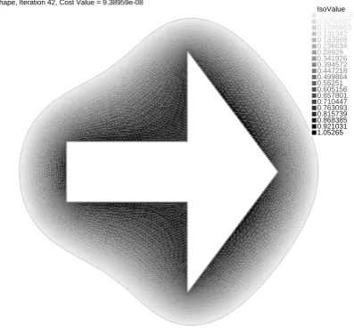
[image:6.595.349.525.277.452.2]IsoValue -0.0529186 0.0260503 0.0786963 0.131342 0.183988 0.236634 0.28928 0.341926 0.394572 0.447218 0.499864 0.55251 0.605156 0.657801 0.710447 0.763093 0.815739 0.868385
0.921031
[image:7.595.86.285.56.243.2]1.05265 Final shape, Iteration 42, Cost Value = 9.38959e-08
Fig. 3. State solution on final shape.
Number of Iterations
0 5 10 15 20 25 30 35 40 45
log
10
J
10-8
10-6
10-4
10-2
100
102
Fig. 4. Histories of the cost functional.
recalculation. Moreover, this new step size is chosen such that there are no reversed triangles within the mesh of the new domain. The iteration loop in the algorithm stops when the stopping criterion J(Ωk) <10−7 is already satisfied. This condition was met after 42 iterations with the resulting optimal shape depicted in Figure 2 with with cost value J(Ω42) = 9×10⁻⁸ as indicated in Figure
3 . The history of the cost functional values are shown in Figure 4. Notice that several fluctuations occur on the values of the cost functional as shown, for instance, in iterations 7, 8 and 9. These fluctuations occur due to the process of updating the step size tk as described above.
V. CONCLUDINGREMARK
We have successfully carried out the computation of the shape derivative of the corresponding cost functional of the tracking Dirichlet problem which is obtained through a reformulation of the exterior Bernoulli free boundary problem in a shape optimiza-tion setting. In particular, we have established the expression for the shape derivative of the cost functional through a Lagrangian formulation coupled with the velocity method. The Lagrangian is expressed as the sum of a utility function plus the equality constraints for the state variable which is actually a mixed-boundary value problem. At this juncture, we mention that another (formal) method that is often used to derive a shape derivative of a functional, which has to be used with caution because it may yield the wrong formula, is due to [12]. This method, known as C´ea’s Lagrange method, uses the same Lagrangian as the minimax formulation.
However, it requires that the shape derivatives of the state and the adjoint equation exist and belong to the solution space of the PDE. Indeed, we may defineG(t, φ, ψ) :=G(Σt, φ, ψ)whereGis given by (7) and assume thatGis sufficiently differentiable with respect to t,φandψ. Since the strong material derivativeu˙ exists inHΓ1,0(Ω)
(cf. [7]), then we may calculate the shape gradient as follows
dJ(Σ;V) = d dtG(t, u
t , p)
t=0
=∂tG(t, u, p)|t=0
| {z }
shape gradient
+∂uG(0,u,p)[ ˙u]
| {z }
adjoint equation
.
The second expression on the right-hand side of the above equation vanishes due to u˙ ∈ H01(Ω), and therefore we are left with
dJ(Σ;V) = ddtG(t, ut, p)t=0. The boundary expression of the shape derivative can be calculated without any difficulty following the line of computations in Section III. Consequently, the computed expression for the shape derivative corroborate the result in [25], and we observe that the shape derivative of the cost functionalJ depends on the normal component of the deformation field V at the free boundaryΣ; that is, there exists a functiongΩ defined on
the free boundaryΣsuch that
dJ(Σ;V) =
∫
Σ
gΩV·νds.
This result agrees with the Hadamard-Zol´esio structure theorem (cf. [31] and [14, Remark 3.2, p. 481]). The fact that we can write the shape derivative of J in terms of a boundary integral allowed us to develop an efficient boundary variation algorithm based on the modified H1 gradient method to numerically solve two concrete examples of the shape optimization problem (2)-(27). Even though shape optimization is, numerically, a very demanding process (cf. [11], [30]), our results show that the proposed iterative algorithm provides an (alternative) efficient numerical procedure in solving the free boundary problem through shape optimization approach.
APPENDIX
We first introduce some notations. Consider a functional
G: [0, τ]×X×Y →R,
for someτ >0 and topological spaces X and Y. For eacht in
[0, τ], we define
g(t) = inf
x∈Xysup∈Y
G(t, x, y) and h(t) = sup
y∈Y
inf
x∈XG(t, x, y)
and the associated sets
X(t) =
{
ˆ
x∈X : sup
y∈Y
G(t,x, yˆ ) =g(t)
}
, (28)
Y(t) =
{
ˆ
y∈Y : inf
x∈XG(t, x,yˆ) =h(t) }
. (29)
To complete the set of notations, we introduce the set of saddle points
S(t) ={(ˆx,yˆ)∈X×Y :g(t) =G(t,x,ˆ yˆ) =h(t)}, (30)
which may be empty. In general, we always have the inequality h(t)≤g(t). Further, for a fixedtin[0, τ], and for all(xt, yt) = (ˆx,yˆ) in X(t)×Y(t), h(t) ≤ G(t, xt, yt) ≤ g(t), and when h(t) =g(t), the set of saddle pointsS(t)is exactlyX(t)×Y(t). Now, the objective of this method is to seek realistic conditions under which the existence of the limit
dg(0) = lim
t↘0
g(t)−g(0)
t
is guaranteed. We are particularly interested on the situation when Gadmits saddle points for alltin[0, τ].
Now, we quote the improved version [14, Thm. 5.1, pp. 556– 559] of the theorem of Correa and Seeger. The result also applies to situations when the state equation admits no unique solution and
IAENG International Journal of Applied Mathematics, 47:4, IJAM_47_4_07
[image:7.595.52.279.284.459.2]the Lagrangian admits saddle points. The proof of this theorem is also given in the said reference.
Theorem 2 (Correa and Seeger, [13]): Let the sets X and Y, the real numberτ >0, and the functional
G: [0, τ]×X×Y →R
be given. Assume that the following assumptions hold: (H1) S(t)̸=∅,0≤t≤τ;
(H2) for all (x, y) ∈ [∪{X(t) : 0≤t≤τ} ×Y(0)] ∪ [X(t)× ∪{Y(t) : 0≤t≤τ}], the partial derivative ∂tG(t, x, y)exists everywhere in[0, τ];
(H3) there exists a topologyTXonX such that for any sequence
{tn: 0< tn≤τ}, tn→t0= 0, there exist anx0∈X(0)
and a subsequence{tnk}of{tn}, and for eachk≥1, there existsxnk∈X(tnk)such that
(i) xnk →x0
in theTX-topology, and (ii) for allyinY(0),
lim inf
t↘0
k→∞
∂tG(t, xnk, y)≥∂tG(0, x0, y); (31)
(H4) there exists a topologyTY onY such that for any sequence
{tn : 0 < tn ≤ τ}, tn →t0 = 0, there existy0 ∈ Y(0)
and a subsequence{tnk}of{tn}, and for eachk≥1, there existsxnk∈X(tnk)such that
(i) ynk →y
0
in theTY-topology, and (ii) for allxinX(0),
lim sup
t↘0
k→∞
∂tG(t, x, ynk)≤∂tG(0, x, y0); (32)
Then, there exists(x0, y0)∈X(0)×Y(0)
such that
dg(0) = inf
x∈X(0)y∈supY(0)∂tG(0, x, y) =∂tG(0, x 0
, y0)
= sup
y∈Y(0)
inf
x∈X(0)∂tG(0, x, y). (33)
Thus(x0, y0)is a saddle point of∂tG(0, x, y)onX(0)×Y(0).
ACKNOWLEDGMENT
This research was done under a project funded by the UP System Emerging Interdisciplinary Research Program (OVPAA-EIDR-C05-015). The authors would like to thank University of the Philippines System and UP Baguio for the support given for the publication of this manuscript.
REFERENCES
[1] B. Abda, F. Bouchon, G. Peichl, M. Sayeh and R. Touzani, “A new formulation for the Bernoulli problem,” in Proceedings of the 5th International Conference on Inverse Problems, Control and Shape Optimization, pp. 1–19, 2010.
[2] R. A. Adams,Sobolev Spaces, Academic Press, London, 1975. [3] H. Azegami, “A solution to domain optimization problems,”Trans of
Japan Soc. of Mech. Engs., Ser. A, vol. 60, pp. 1479–1486, 1994. (in Japanese).
[4] H. Azegami and Z. Q. Wu, “Domain optimization analysis in linear elastic problems: Approach using traction method”,JSME Int. J. Ser. A, vol. 39, no.2, pp. 272–278, 1996.
[5] H. Azegami, S. Fukumoto and T. Aoyama, “Shape optimization of continua using nurbs as basis functions”,Struct. Multidiscipl. Optimiz., vol. 47, no. 2, pp. 247–258, 2013.
[6] H. Azegami, L. Zhou, K. Umemura and N. Kondo, “Shape optimiza-tion for a link mechanism”,Struct. Multidiscipl. Optimiz., vol. 48, pp. 115–125, 2013.
[7] J. B. Bacani and G. H. Peichl, “On the first-order shape derivative of the Kohn-Vogelius cost functional of the Bernoulli problem,”Abstr. Appl. Anal., vol. 2013, Article ID 384320, 19 pages, 2013. [8] J. B. Bacani and G. H. Peichl, “The second-order Eulerian derivative of
a shape functional of a free boundary problem,”IAENG International Journal of Applied Mathematics, vol. 46, no. 2, pp. 425–436, 2016. [9] Z. Belhachmi and H. Meftahi, “Shape sensitivity analysis for an
interface problem via minimax differentiability,”Appl. Math. Comput., vol. 219, pp. 6828–6842, 2013.
[10] A. Boulkhemair, A. Nachaoui and A. Chakib, “A shape optimization approach for a class of free boundary problems of Bernoulli type,”
Appl. Math., vol. 58, no.2, pp. 205–231, 2013.
[11] F. D. Calvo, V. M. Chapela, M. J. Percino and L. Trinidad, “Solar panel optimization of a parabolic channel to generate electrical energy,” Lecture Notes in Engineering and Computer Science: Proceedings of The World Congress on Engineering 2013, WCE 2013, 3-5 July, 2013, London, U.K., pp. 496-500.
[12] J. C´ea, “Conception optimale ou identification de formes, calcul rapide de la derivee dircetionelle de la fonction cout,”Math. Mod. Numer. Anal., vol. 20, pp. 371–402, 1986.
[13] R. Correa and A. Seeger, “Directional derivative of a minimax func-tion,”Nonlinear Anal Theory Methods Appl., vol. 9, pp. 13–22, 1985 [14] M. C. Delfour and J.-P. Zol´esio, “Shapes and Geometries: Metrics, Analysis, Differential Calculus, and Optimization, 2nd ed.,”Adv. Des. Control 22, SIAM, Philadelphia,2011.
[15] M. C. Delfour and J.-P. Zol´esio, “Velocity method and Lagrangian formulation for the computation of the shape Hessian,” SIAM J. Control Optim., vol. 29, no. 6, pp. 1414–1442, 1991.
[16] I. Ekeland and R. Temam, “Convex Analysis and Variational Prob-lems,” North-Holland Publishing Co., Amsterdam, 1976. Translated from the French, Studies in Mathematics and its Applications, Vol. 1. [17] M. Flucher and M. Rumpf, “Bernoulli’s free-boundary problem, qual-itative theory and numerical approximation,”J. Reine Angew. Math., vol. 486, pp. 165–204, 2003.
[18] A. Friedman, “Free boundary problems in science and technology,”
Notices of the AMS, vol. 47, pp. 854–861, 2000.
[19] Z. Gao and Y. Ma, “Shape gradient of the dissipated energy functional in shape optimization for the viscous incompressible flow,” Appl. Numer. Math., vol. 58, pp. 1720–1741, 2008.
[20] Z. Gao, Y. Ma and H. W. Zhuang, “Shape Hessian for generalized Oseen flow by differentiability of a minimax: A Lagrangian approach,”
Czechoslovak Math. J., vol. 57, no. 3, pp. 987–1011, 2007. [21] D. Gilbarg and N. S. Trudinger,Elliptic Partial Differential Equations
of Second Order, Springer, Berlin, Germany, 1983.
[22] J. Haslinger and R. A. E. M¨akinen,Introduction to Shape Optimiza-tion: Theory, Approximation, and Computation, Advances in Design and Control, Society for Industrial and Applied Mathematics, 2003. [23] J. Haslinger, K. Ito, T. Kozubek, K. Kunisch and G. Peichl, “On
the shape derivative for problems of Bernoulli type,”Interfaces Free Bound., vol. 1, pp. 317–330, 2009.
[24] F. Hecht, “New development in FreeFem++”,J. Numer. Math., vol. 20, no. 3-4, pp 251–265, 2012.
[25] K. Ito, K. Kunisch and G. Peichl, “Variational approach to shape derivative for a class of Bernoulli problem,”J. Math. Anal. App., vol. 314, pp.126–149, 2006.
[26] A. Laurain and H. Meftahi, “Shape and parameter reconstruction for the Robin inverse problem,”J. Inverse Ill-Posed Probl., vol. 24, no. 6, pp. 642–662, 2016.
[27] J. L. Lions,Optimal control of systems governed by partial differential equations,Berlin Heidelberg: Springer-Verlag, 1971.
[28] H. Meftahi, “Stability analysis in the inverse Robin transmission problem,”Math. Methods Appl. Sci., vol. 40, no. 7, pp. 2505–2521, 2017.
[29] H. Meftahi and J. P. Zol´esio, “Sensitivity analysis for some inverse problems in linear elasticity via minimax differentiability,”Appl. Math. Model., vol. 39, pp. 1554–1576, 2015.
[30] D. Vucina, Z. Lozina and I. Pehnec, “Reverse engineering with shape optimization using workflow-based computation and distributed computing,” Lecture Notes in Engineering and Computer Science: Proceedings of The World Congress on Engineering 2009, WCE 2009, 1-3 July, 2009, London, U.K., pp. 789–794.
[31] J. Sokolowski and J.-P. Zol´esio,Introduction to Shape Optimization, Springer, Berlin, Germany, 1991.