Permanence and Uniform Asymptotical Stability in
Consumer-Resource System with Mutual
Interference on Time Scales
Yongyan Yang and Tianwei Zhang
Abstract—This paper is concerned with a consumer-resource system described by a mutual interference model with feedback controls on time scale. By using time scale calculus theory and differential inequality, some verifiable conditions are obtained for the permanence of the above system. Further, by some important inequalities, the uniform asymptotical stability of the model have been studied. An example and numerical remarks are provided to illustrate the main results of this paper. Finally, a conclusion is also given to discuss how the feedback control and mutual interference of the system influence the permanence.
Index Terms—Consumer-resource; permanence; feedback control; mutual interference; asymptotical stability.
I. INTRODUCTION
I
T is well known that the dynamic relationship between predator and prey has been extensively studied in both economy and mathematical ecology by several scholars[1-7]. However, there were few papers considering the mutual interference until Hassell introduced it as constant m(0 < m≤1) in 1971, see paper [8-10] for more details. On the basis of the results in[8], further research was done by Feng Zhang in[11], the system as follows:{
x′(t) =x(t)[a(t)−b(t)xθ(t)]−a(t)x(t)ym(t),
y′(t) =y(t)[d(t)−e(t)yx((tt))], (1.1)
where a(t) andd(t) stand for the intrinsic growth rates of the prey and the predator at timet, respectively, ab((tt)) is the carrying capacity of the prey in the absence of predation,
e(t)is a measure of the food quantity that prey provides and converted to predator birth, 0< m, θ≤1.
On the other hand, the consumer-resource(C-R) interac-tion, which has become a central principle for understanding interspecific interactions, play a very important role and received much attention [12-16]. Motivated by the above reasons and based on the system (1.1), we present a specific consumer-resource system described by a model with mutual interference and feedback control:
N1′(t) = N1(t)[a(t)−b(t)Nθ
1(t)−c(t)N2m(t)]
−α(t)u(t),
u′(t) = −f1(t)u(t) +p1(t)N1(t−τ), N2′(t) = N2(t)[d(t)−e(t)
N2(t)
N1(t)]−β(t)v(t),
v′(t) = −f2(t)v(t) +p2(t)N2(t−τ),
(1.2)
Manuscript received June 29, 2018; revised October 27, 2018. Yongyan Yang is with College of Mathematical and Physical Sciences, Anyang University, Anyang 455000, China. ([email protected]).
Tianwei Zhang is with the City College, Kunming University of Science and Technology, Kunming 650051, China. ([email protected]).
Correspondence author: Tianwei Zhang. ([email protected]).
where N1(t) and N2(t) represent the population density of the resource and the consumer at time t, respectively.
a(t)andd(t)denote the intrinsic growth rate of the resource and consumer, ab((tt)) stands for its carrying capacity when in isolation from the resource,c(t)N1(t)represents the decrease
in the growth of the resourcee(t) is a measurement of consumption of resource,0< m, θ≤1,u(t)andv(t)denote the feedback control variables. Ifm= 1, there is no mutual interference between the consumer and resource, hence in this paper we just consider the system with 0 < m < 1. But any economy models are set up in either continuous or discrete model. So, time scale approach is more flexible and realistic. Motivated by the above reasons and based on the system (1.2), we present a specific consumer-resource system described by a model with mutual interference and feedback control on time scale:
N1∆(t) = a(t)−b(t) exp{θN1(t)}
−c(t) exp{mN2(t)} −α(t)u(t), u∆(t) = −f
1(t)u(t) +p1(t) exp{N1(t−τ)}, N∆
2 (t) = d(t)−e(t) exp{N2(t)−N1(t)} −β(t)v(t), v∆(t) = −f
2(t)v(t) +p2(t) exp{N2(t−τ)},
(1.3)
where all the variables have the same meaning of the system (1.2) and are rd-continuous positive. Clearly, if we choose
T=R, then the system (1.3) can be reduced to(1.2). System (1.3) satisfies the initial values:
N1(s) =φ(s)≥0, s∈[−τ,0)T,
φ∈Crd([−τ,0)T, R), φ(0)>0;
N2(s) =ϕ(s)≥0, s∈[−τ,0)T,
ϕ∈Crd([−τ,0)T, R), ϕ(0)>0;
u(0)>0, v(0)>0.
This article is organized as follows: Section 2 provides some definitions and notations, we show the permanence of the system (1.3) in section 3, Finally we give some examples.
II. PRELIMINARIES
In this section, we shall first recall some basic definitions and lemmas on time scales, which can be found in [17].
Definition 1. ([17])A time scaleTis an arbitrary nonempty closed subset of the real numbersR, the set T inherits the standard topology ofR.
Definition 2. ([17]) The forward and the backward jump operatorsσ, ρ:T→ T, and the graininessµ: T→R+ = [0,∞)are defined, respecting, by
σ(t) = inf{s∈T:s > t},
ρ(t) = sup{s∈T:s < t},
IAENG International Journal of Applied Mathematics, 49:3, IJAM_49_3_10
µ(t) =σ(t)−t f or t∈T.
If σ(t) = t, then t is called dense (otherwise: right-scattered), and if ρ(t) = t, then t is called left-dense (otherwise: left-scattered).
Definition 3. ([17]) A function f : T → R is said to be rd-continuous if it is continuous at right-dense points in T and its left-sided limits exists (finite) at left-dense point in
T. The set of rd-continuous function f : T → R will be denoted by Crd(T,R).
Definition 4. ([17])Assumef :T→Ris a function and let
t∈T. Then we define f∆(t)to be the number (provided it exists) with the property that given anyϵ >0, for alls∈U, there is a neighborhood U oft such that
|f(σ(t))−f(s)−f∆(t)(σ(t)−s)| ≤ϵ|σ(t)−s|
In this case,f∆(t)is called the delta (or Hilger) derivative of
f att. Moreover,f is said to be delta or Hilger differentiable on T if f∆(t) exists for all t ∈ T. The set of functions f : T → R that are differentiable and those delta-derivative are rd-continuous functions is denoted by C1
rd =
C1
rd(T) =C
1
rd(T,R).
Definition 5. ([17]) A function F : T → R is called a antiderivative of f :T→R providedF∆(t) =f(t) for all
t, s∈T. Then we write
∫ s
r
f(t)∆t=F(s)−F(r).
Lemma 1. ([17])Every rd-continuous function has an an-tiderivative and every continuous function is rd-continuous.
Lemma 2. ([17]) Assume−a∈R+, x(t
0)>0, t0∈T.
(i) Ifx∆(t)≤b−ax(t), whent≥t0, one has
x(t)≤x(t0)e(−a)(t, t0) + b
a(1−e(−a)(t, t0)),
particularly, when a >0, b >0, one has
lim
t→+∞supx(t)≤ b a;
(ii) Ifx∆(t)≥b−ax(t), whent≥t
0, one has
x(t)≥x(t0)e(−a)(t, t0) + b
a(1−e(−a)(t, t0)),
particularly, when a >0, b >0, one has
lim
t→+∞infx(t)≥ b a.
Let f be a continuous bounded function on T and set
fu = sup
t∈T
f(t), fl = inf
t∈Tf(t), one assumes the following
hypothesis holds:
(H1) a(t), b(t), c(t), d(t), e(t), fi(t), pi(t)α(t), β(t) are
all positive and rd-continuous(i= 1,2);
(H2) du+el(M1−1)>0;
(H3) au−bl>0.
Definition 6. For any solution(N1(t), u(t), N2(t), v(t))T of
system (1.3), exist mi, li, Mi, Li>0(i= 1,2) , such that:
m1≤ lim
t→+∞infN1(t)≤t→lim+∞supN1(t)≤M1,
m2≤ lim
t→+∞infN2(t)≤t→lim+∞supN2(t)≤M2, l1≤ lim
t→+∞infu(t)≤t→lim+∞supu(t)≤L1, l2≤ lim
t→+∞infv(t)≤t→lim+∞supv(t)≤L2.
III. PERMANENCE
This section studies the permanence of system (1.3), for convenience we put:
M1= au−bl
θbl , L1=
pu
1exp{M1} fl
1 ,
M2= d
u+el(M1−1)
el , L2=
pu
2exp{M2} fl
2
m1=1
θln
al−cuexp{mM2} −αuL1
bu , l1=
pl1exp{m1} fu
1
m2=m1+ lnd
l−βuL2
eu , l2=
pl2m2 fu
2 .
Theorem 1. Suppose the system (1.3) satisfies the conditions
(H1)-(H3)and the following conditions:
(H4) al−cuexp{mM
2} −αuL1>0,
(H5) dl−βuL2>0,
then the system (1.3) is permanence.
Proof: (1)From the first equation of the system (1.3), it follows that
N1∆(t)≤ a(t)−b(t) exp{θN1(t)} ≤ a(t)−b(t)(1 +θN1(t))
≤ au−bl−θblN1(t). (3.1)
Applying lemma 2.2 and condition (H3) to (3.1), we obtain
lim
t→+∞supN1(t)≤ au−bl
θbl =M1. (3.2)
From (3.2), we know that there exists a t1 ∈ T enough large such thatN1(t)≤M1, t≥t1 >0. Then, there exists
t2=t1+τ such that, for anyt≥t2>0,N1(t−τ)≤M1.
By the second equation of the system (1.3), we get:
u∆(t)≤ −f1lu(t) +pu1exp{M1}, (3.3)
in view of Lemma 2.2, it follows from (3.3) that
lim
t→+∞supu(t)≤
pu1exp{M1} fl
1
=L1. (3.4)
Similarly, by the third equation of system (1.3), we have
N2∆(t)≤ d(t)−e(t)(1 +N2(t)−N1(t))
≤ du−el−elN2(t) +elM1. (3.5)
It follows from Lemma 2.2 and condition (H2) that
lim
t→+∞supN2(t)≤
du+el(M1−1)
el =M2. (3.6)
With (3.6) we know that there exists a t3 ∈Tsuch that, for any t ≥ t3 > 0, N2(t) ≤ M2. Therefore, there exists
t4=t3+τ,for anyt≥t4>0, such thatN2(t−τ)≤M2.
Then, we can get the following results easily:
v∆(t)≤ −f2lv(t) +p
u
2exp{M2}, (3.7)
IAENG International Journal of Applied Mathematics, 49:3, IJAM_49_3_10
lim
t→+∞supv(t)≤
pu2exp{M2} fl
2
=L2. (3.8)
(2) In view of (3.4), there exists at5∈T, for anyt≥t5>
0, such that u(t) ≤L1. Let t6 = max{t3, t5}, for t > t6,
we getN2≤M2, u(t)≤L1 and
N1∆(t)
≥a(t)−b(t) exp{θN1(t)} −c(t) exp{mN2(t)} −α(t)L1
≥al−buexp{θN1(t)} −cuexp{mM2} −αuL1. (3.9)
Hence, when t≥t5>0, we get
al−buexp{θN1(t)} −cuexp{mM2} −αuL1≤0(3.10).
Otherwise, suppose that exists t′ ≥t5 such that
al−buexp{θN1(t)} −cuexp{mM2} −αuL1>0,
and for t∈[t5, t′)T, we get
al−buexp{θN1(t)} −cuexp{mM2} −αuL1≤0.
So
N1(t′)<
1
θln
al−cuexp{mM
2} −αuL1
bu ,
for t∈[t5, t′)T, we obtain that
N1(t′)≥
1
θln
al−cuexp{mM
2} −αuL1
bu , x
∆(t′)<0,
which conflicts with known conditions.
Therefore, (3.10) is establishment, hence, fort≥t5,
N1(t)≥
1
θln
al−cuexp{mM
2} −αuL1 bu =m1,
thus
lim
t→+∞infN1(t)≥m1. (3.11)
From the second equation of system (1.3), we obtain that:
u∆(t)≥ −f1uu(t) +pl1exp{m1}.By Lemma 2.2, we have:
lim
t→+∞infu(t)≥ pl
1exp{m1} fu
1
=l1. (3.12)
Similarly, we can get:
lim
t→+∞infN2(t) ≥m1+ ln
dl−βuL2
eu =m2, (3.13)
lim
t→+∞infv(t) ≥ pl
2m2 fu
2
=l2. (3.14)
With equation (3.2),(3.4),(3.6),(3.8) and (3.11)-(3.14), the system (1.3) is permanence.
This completes the proof.
IV. UNIFORM ASYMPTOTICAL STABILITY
The main result of this paper concerns the uniformly asymptotically stable of system(1.3).
Theorem 2. Letτ= 1in system(1.3). Suppose(H1)-(H5)
and the following condition hold:
(H6) there exists a constantµ such that
θbleθm1−eueM1+M2−2m1−pu
1e
M1> µ,
elem2−M1−mcuemM2−pu
2e
M2 > µ,
f1l−αu> µ, f2l−βu> µ,
whereM1,M2,m1 andm2are defined as that in Theorem
1. Then system(1.3)is uniformly asymptotically stable.
Proof: Suppose that Z(t) =
(N1(t), N2(t), u(t), v(t))T and Z∗(t) =
(N1∗(t), N2∗(t), u∗(t), v∗(t))T are any two solutions of
system(1.3).
In view of system(1.3), we have
[N1(t)−N1∗(t)] ∆
= −b(t)[exp{θN1(t)} −exp{θN1∗(t)}] −c(t)[exp{mN2(t)} −exp{mN2∗(t)}] −α(t)[u(t)−u∗(t)],
which implies that
D+|N1(t)−N1∗(t)|∆ ≤ −θbleθm1|N1(t)−N1∗(t)|
+mcuemM2|N2(t)−N∗
2(t)|
+αu|u(t)−u∗(t)|,
similarly,
D+|N2(t)−N2∗(t)|
∆ ≤ −elem2−M1|N
2(t)−N2∗(t)|
+eueM1+M2−2m1|N1(t)−N∗
1(t)|
+βu|v(t)−v∗(t)|,
D+|u(t)−u∗(t)|∆ ≤ −f1l|u(t)−u∗(t)|
+pu1eM1|N1(t)−N∗
1(t)|,
D+|v(t)−v∗(t)|∆ ≤ −f2l|v(t)−v∗(t)| +pu2eM2|N
2(t)−N2∗(t)|.
SetV(t) =|N1(t)−N1∗(t)|+|N2(t)−N2∗(t)|+|u(t)− u(t)|+|v(t)−v(t)|. Then
D+V(t)∆
≤ [−θbleθm1+eueM1+M2−2m1+pu
1e
M1]|N1(t)−N∗
1(t)|
+[−elem2−M1+mcuemM2+pu
2e
M2]|N
2(t)−N2∗(t)|
+[−f1l+αu]|u(t)−u∗(t)|+ [−f2l+βu]|v(t)−v∗(t)|
≤ −µV(t). (4.1)
Therefore, V is non-increasing. Integrating (4.1) from 0
totleads to
V(t) +µ ∫ t
0
V(s) ds≤V(0)<+∞, ∀t≥0,
that is, ∫
+∞
0
V(s) ds <+∞,
which implies that
lim
s→+∞|N1(t)−N
∗
1(t)|= lim
s→+∞|N2(t)−N
∗
2(t)|= 0,
lim
s→+∞|u(t)−u
∗(t)|= lim
s→+∞|v(t)−v
∗(t)|= 0.
Thus, system (1.3) is uniformly asymptotically stable. This completes the proof.
IAENG International Journal of Applied Mathematics, 49:3, IJAM_49_3_10
V. AN EXAMPLE AND NUMERICAL SIMULATIONS
Example 1. Let T = R, considering the coefficients of system (1.2) as follows:
a= 3.2 + 0.4 sin 2t, b= 1.1 + 0.2 sint, c= 0.08,
d= 1.5 + 0.2 cos 2t, e= 0.9 + 0.3 sint, m= 0.02, θ= 0.8,
f1= 1.8 + 0.6 sin 3t, f2= 2.5 + 0.3 cos 3t, α= 0.015,
p1= 0.3 + 0.2 sin 2t, p2= 0.4 + 0.2 cos 2t, β= 0.013.
By calculating, it satisfies the conditions (H1)-(H5), in view of Theorem 3.1, we obtain that system (1.2) is permanent. This following figure establishes the dynamic behavior of system (1.2).
0 10 20 30 40 50 60 0
1 2 3 4 5 6 7 8 9 10
t
N1
(t),N
2
(t),u,v
N 1(t) N
2(t) u v
Fig. 1 Dynamic behavior of system (1.2) with the initial condition (N1(0), u(0), N2(0), v(0)) = (1.5,1.3,2.1,1.1)T, andτ= 0.
Remark 1. Let θ = 1, m = 1, τ = 0 in system (1.3) and
T=R, the system (1.3) can be simplified as follows:
N1′(t) = N1(t)[a(t)−b(t)N1(t)−c(t)N2(t)]
−α(t)u(t),
u′(t) = −f1(t)u(t) +p1(t)N1(t), N2′(t) = N2(t)[d(t)−e(t)N2(t)
N1(t)]−β(t)v(t),
v′(t) = −f2(t)v(t) +p2(t)N2(t),
(5.1)
we can get the system (4.1) is permanent by using theorem 3.1, and if we let the coefficients of system (4.1) and (1.2) to be the same, we can use figure 2 to establish the dynamic of system (4.1).
0 10 20 30 40 50 60 0
1 2 3 4 5 6 7
t
N1
(t),N
2
(t),u,v
N 1(t) N
2(t) u v
Fig. 2 Dynamic behavior of system (1.2)with the initial condition (N1(0), u(0), N2(0), v(0)) = (1.5,1.3,2.1,1.1)T, and τ= 0.
Remark 2. Suppose that system (1.3) without feedback control, and let θ = 1, m = 1, τ = 0, we can get the following system:
{ N∆
1 (t) =a(t)−b(t) exp{N1(t)} −c(t) exp{N2(t)}, N∆
2 (t) =d(t)−e(t) exp{N2(t)−N1(t)}.
(5.2)
Suppose condition (H1)-(H3) hold, then the system (3.16) is permanent. Suppose further that T = R and all the coefficients of system (3.16) to be the same with example (3.1), we use figure 3 to establish the dynamic.
0 10 20 30 40 50 60 1.5
2 2.5 3 3.5 4 4.5 5 5.5 6 6.5
t
N1
(t),N
2
(t)
N1(t) N
2(t)
Fig. 3 Dynamic behavior of system (3.16) with the initial condi-tion(N1(0), N2(0)) = (1.5,2.1)T.
By comparing figure 2 and figure 3, we can obtain that the feedback control is harmless to the permanence of system.
Remark 3. Suppose that system (1.3) without feedback control but has mutual interference just as follows:
{ N∆
1 (t) =a(t)−b(t) exp{θN1(t)} −c(t) exp{mN2(t)}, N∆
2 (t) =d(t)−e(t) exp{N2(t)−N1(t)},
With the condition (H1)-(H3), we get this system is perma-nence. LetT=R, the above system can be simplified to be
IAENG International Journal of Applied Mathematics, 49:3, IJAM_49_3_10
[image:4.595.318.534.63.235.2] [image:4.595.61.278.367.543.2] [image:4.595.314.536.441.613.2]as follows:
{
N1′(t) =N1(t)[a(t)−b(t)N1θ(t)]−c(t)N1(t)N2m(t), N2′(t) =N2(t)[d(t)−e(t)N2(t)
N1(t)].
(5.3)
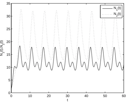
The coefficients a(t), b(t), c(t), d(t), e(t) and the initial condition N1(0), N2(0) are the same to example 1, let
θ = 0.5, m = 0.6 and θ = 0.3, m = 0.8 in addition, by calculating, we know they satisfy all the condition of theorem (3.1), the figures ia as follows:
0 10 20 30 40 50 60 0
2 4 6 8 10 12 14 16 18 20
t
N1
(t),N
2
(t)
N1(t) N
2(t)
Fig. 4 The dynamic behavior of system 4.3 withθ = 0.5, m= 0.6.
0 10 20 30 40 50 60 0
5 10 15 20 25 30 35
t
N1
(t),N
2
(t)
N 1(t) N
2(t)
Fig. 5 The dynamic behavior of system 4.3 withθ = 0.3, m= 0.8.
By comparing with the figure 4 and figure 5, we can get the mutual interference is harmless for the permanence of the system but has a great influence on the population density of the resource and consumer.
VI. CONCLUSION
Make a comparison with our results, from the remark 1-3, we can easy to see that the C-R system (1.3) can maintain persistence with the appropriate condition, feedback control and mutual interference have less influence on the perma-nence of the C-R system, while the latter has a great influence
on the population density of the resource and consumer. In addition system (1.3) can be seen a generalization of paper [11].
REFERENCES
[1] L. Li, B. Du, ”Global asymptotical stability in a stochastic predator-prey system with variable delays”,IAENG International Journal of Applied Mathematics, vol. 46, no.2, pp241-246, 2016.
[2] L.L. Wang, P.L. Xie, ”Permanence and extinction of delayed stage-structured predator-prey system on time scales”,Engineering Letters, vol. 25, no.2, pp147-151, 2017.
[3] L.L. Wang, ”Dynamic analysis on an almost periodic predator-prey model with impulses effects”,Engineering Letters, vol. 26, no.3, pp333-339, 2018.
[4] H.J. Zhou, M. Liu, ”Analysis of a stochastic predator-prey model in polluted environments”, IAENG International Journal of Applied Mathematics, vol. 46, no.4, pp445-456, 2016.
[5] T.W. Zhang, Y.K. Li, Y. Ye, ”On the existence and stability of a unique almost periodic solution of Schoener’s competition model with pure-delays and impulsive effects”,Commun. Nonlinear Sci. Numer. Simulat.
17, 1408-1422, 2012.
[6] Y.K. Li, T.W. Zhang, ”Permanence and almost periodic sequence solution for a discrete delay logistic equation with feedback control”,
Nonlinear Anal. Real World Appl.12, 1850-1864, 2011.
[7] T.W. Zhang, Y.K. Li, Y. Ye, ”Persistence and almost periodic solutions for a discrete fishing model with feedback control”,Commun. Nonlinear Sci. Numer. Simul.16, 1564-1573, 2011.
[8] M.P. Hessel, ” Mutual interference between searching insect parasites”,
Anim Ecol.40, 473-486, 1971.
[9] P.H. Leslie, ”Some further notes on the use of matrices in population mathematics”,Biometrika35, 213-245, 1948.
[10] M.P. Hessel, ”Density dependence in single-species population”,Anim Ecol.44, 283-295, 1975.
[11] F. Zhang, W.C. Chen, Y.M. Zhang, ”Qualitative analysis of a Leslie predator-prey system with mutual interference”, Biomathematics 29, 169-173, 2014.
[12] J. N. Holland, D. L. Deangelis, ”Consumer-resource theory predicts dynamic transitions between outcomes of interspecific interactions”,
Ecol. Lett.12, 1357-1366, 2009.
[13] Y.Q. Li, T.W. Zhang, ”Almost periodic dynamics in a nonautonomous bi-directional consumer-resource system with time delays”,Comp. Appl. Math.35, 559-577, 2016.
[14] Z.H. Liu, P. Magel, S.G. Ruan, ”Oscillations in Age-Structured Models of Consumer-Resource Mutualisms”,Discrete and Continuous Dynam-ical Systems-Series, 21, 537-555, 2016.
[15] Y.S. Wang, D.L. Deangelis, J.N. Holland, ”Uni-directional consumer-resource theory characterizing transitions of interaction outcomes”,
Ecol. Comp. 4, 249-257, 2011.
[16] J.N. Holland, D.L. Deangelis, ”A consumer-resource approach to the density-dependent population dynamics of mutualism”,Ecol.5, 1286-1295, 2010.
[17] Bohner, M. Peterson, ”Dynamic equations on time scales, an Intro-duction with applications”,Birkhauser, Boston2001.