A hybrid MLP CNN classifier for very fine resolution remotely sensed image classification

1

A hybrid MLP-CNN classifier for very fine resolution

1

remotely sensed image classification

2

Ce Zhang 1, *, Xin Pan 2, 3, Huapeng Li 2, Andy Gardiner 4, Isabel Sargent 4, Jonathon 3

Hare 5_{, Peter M. Atkinson} 1, * 4

1 _{Lancaster Environment Centre, Lancaster University, Lancaster LA1 4YQ, UK;} 2 _{Northeast Institute} 5

of Geography and Agroecology, Chinese Academic of Science, Changchun 130102, China; 3 _{School of} 6

Computer Technology and Engineering, Changchun Institute of Technology, 130021 Changchun,

7

China; 4 _{Ordnance Survey, Adanac Drive, Southampton SO16 0AS, UK;} 5 _{Electronics and Computer} 8

Science (ECS), University of Southampton, Southampton SO17 1BJ, UK

9

Abstract The contextual-based convolutional neural network (CNN) with deep

10

architecture and pixel-based multilayer perceptron (MLP) with shallow structure are

11

well-recognized neural network algorithms, representing the state-of-the-art deep

12

learning method and the classical non-parametric machine learning approach,

13

respectively. The two algorithms, which have very different behaviours, were

14

integrated in a concise and effective way using a rule-based decision fusion approach

15

for the classification of very fine spatial resolution (VFSR) remotely sensed imagery.

16

The decision fusion rules, designed primarily based on the classification confidence

17

of the CNN, reflect the generally complementary patterns of the individual

18

classifiers. In consequence, the proposed ensemble classifier MLP-CNN harvests the

19

complementary results acquired from the CNN based on deep spatial feature

20

representation and from the MLP based on spectral discrimination. Meanwhile,

21

limitations of the CNN due to the adoption of convolutional filters such as the

22

uncertainty in object boundary partition and loss of useful fine spatial resolution

23

detail were compensated. The effectiveness of the ensemble MLP-CNN classifier

24

was tested in both urban and rural areas using aerial photography together with an

25

additional satellite sensor dataset. The MLP-CNN classifier achieved promising

26

performance, consistently outperforming the pixel-based MLP, spectral and

textural-27

based MLP, and the contextual-based CNN in terms of classification accuracy. This

28

research paves the way to effectively address the complicated problem of VFSR

29

image classification.

30

Keywords: convolutional neural network; multilayer perceptron; VFSR remotely

31

sensed imagery; fusion decision; feature representation

2 1. Introduction

33

With the rapid development of modern remote sensing technologies, a large quantity of 34

very fine spatial resolution (VFSR) images is now commercially available. These 35

VFSR images, typically acquired at sub-metre spatial resolution, have opened up many 36

opportunities for new applications (Zhong et al., 2014), for example, urban land use 37

retrieval (Mathieu et al., 2007; Shi et al., 2015), precision agriculture (Ozdarici-Ok et 38

al., 2015; Zhang and Kovacs, 2012), and tree crown delineation (Ardila et al., 2011; 39

Yin et al., 2015). However, despite the presence of a rich spatial data content (Huang 40

et al., 2014), the information conveyed by the imagery is conditional upon the quality 41

of the processing (Längkvist et al., 2016). With fewer spectral channels in comparison 42

with coarse or medium spatial resolution remotely sensed data, it can be challenging to 43

differentiate subtle differences amongst similar land cover types (Powers et al., 2015). 44

Meanwhile, objects of the same class may exhibit strong spectral heterogeneity due to 45

differences in age, level of maintenance and composition as well as illumination 46

conditions (Demarchi et al., 2014), which might be further complicated by the 47

scattering of peripheral ground objects (Chen et al., 2014). As a consequence, such high 48

intra-class variability and low inter-class disparity make automatic classification of 49

VFSR images a challenging task. 50

Ever since the advent of VFSR imagery, tremendous efforts have been made to develop 51

robust and accurate, automatic image classification methods. Among these, machine 52

learning is currently considered as the most promising and evolving approach (Zhang 53

et al., 2015). Popular pixel-based machine learning algorithms, such as Multilayer 54

Perceptron (MLP), Support Vector Machine (SVM) and Random Forest (RF), have 55

drawn considerable attention in the remote sensing community (Attarchi and Gloaguen, 56

2014; Yang et al., 2012; Zhang et al., 2015). The MLP, as a typical non-parametric 57

neural network classifier, is designed to learn the nonlinear spectral feature space at the 58

pixel level irrespective of its statistical properties (Atkinson and Tatnall, 1997; Foody 59

and Arora, 1997; Mas and Flores, 2008). The MLP has been used widely in remote 60

sensing applications, including VFSR-based land cover classification (e.g. Del Frate et 61

al., (2007), Pacifici et al. (2009)). The MLP algorithm is mathematically complicated 62

yet can be simple in model architecture (e.g., a shallow classifier with one or two feature 63

representation levels). At the same time, a pixel-based MLP classifier does not consider, 64

3

with unprecedented spatial detail. In essence, the MLP (and related algorithms, e.g. 66

SVM, RF, etc.) is a pixel-based classifier with shallow structure (one or two layers) 67

(Chen et al., 2016), where the membership association of a pixel for each class is 68

predicted. 69

Recent advances in neuroscience have shown that deep feature representations can be 70

learned hierarchically from simple concepts such as oriented edges to higher-level 71

complex patterns such as textures, segments, parts and objects (Arel et al., 2010). This 72

discovery motivated the breakthrough of the so-called “deep learning” methods that 73

represent the state-of-the-art in a variety of domains, including target detection (Chen 74

et al., 2016; Tang et al., 2015), image recognition (Farabet et al., 2013; Krizhevsky et 75

al., 2012) and robotics (Bezak et al., 2014; Lenz et al., 2015; Yu et al., 2013), amongst 76

others. The convolutional neural network (CNN), a well-established deep learning 77

approach, has produced excellent results in the field of computer vision and pattern 78

recognition (Schmidhuber, 2015), such as for visual recognition (Farabet et al., 2013; 79

Krizhevsky et al., 2012), image retrieval (X. Yang et al., 2015) and scene annotation 80

(Othman et al., 2016). 81

In the remote sensing domain, CNNs have been studied actively and shown to produce 82

state-of-the-art results over the past few years, focusing primarily on object detection 83

(Dong et al., 2015) or scene classification (Hu et al., 2015a; Zhang et al., 2016). Recent 84

studies further explored the feasibility of CNNs for the task of remotely sensed image 85

classification. For example, Yue et al., (2016) utilized spatial pyramid pooling to learn 86

multi-scale spatial features from hyperspectral data, Chen et al. (2016) introduced a 3D 87

CNN to jointly extract spectral–spatial features, thus, making full use of the continuous 88

hyperspectral and spatial spaces. In terms of the classification of multi- and 89

hyperspectral imagery, a deep CNN model was formulated through a greedy layer-wise 90

unsupervised pre-training strategy (Romero et al., 2016), whereas an image pyramid 91

was built up through upscaling the original image to capture the contextual information 92

at multiple scales (Zhao and Du, 2016). For VFSR image classification, CNN models 93

with varying contextual input size were constructed to learn multi-scale features while 94

preserving the original fine resolution information (Längkvist et al., 2016). All of the 95

above-mentioned work applied CNNs with contextual patches as their inputs, and 96

demonstrated the robustness and effectiveness in spatial feature representations with 97

4

CNN as a classifier itself have not been studied thoroughly. In particular, the CNN, as 99

a contextual classifier with deep structures (Szegedy et al., 2015), explores the complex 100

spatial patterns hidden in the image that are not seen by representation in its shallow 101

counterparts, whereas it may overlook certain information in spectral space observed 102

by pixel-based classifiers. Moreover, uncertainties may appear in object boundaries due 103

to the usage of convolutional filters of the CNN. These issues deserve further 104

investigation. 105

Any single set of features (e.g., spectral only) or a specific classifier (e.g., pixel-based 106

only) is unlikely to achieve the highest classification accuracies for VFSR imagery 107

because the result is conditional upon both spectral and spatial information. In this 108

context, two categories of spectral and spatial information were fused for classification 109

or handled with a classifier ensemble. Information fusion can be realized by stacking 110

the spatial and spectral information as feature bands. However, this does not allow the 111

specification of the relative influence of the extracted features (Wang et al., 2016). 112

Others proposed integrative algorithms considering the spatial and spectral features at 113

the same time. For example, Fauvel et al., (2012) proposed a composite kernel-based 114

SVM with spectral and spatial kernels applied simultaneously. However, the spatial 115

kernel summarizes only basic information (e.g. median) of the spatial neighbourhood 116

(Wang et al., 2016). 117

In terms of classifier ensemble technology, two strategies, namely “multiple classifier 118

systems” (Benediktsson, 2009) and “decision fusion” (Fauvel et al., 2006) are 119

employed. Multiple classifier systems are based on the manipulation of training sample 120

sets, including boosting (Freund et al., 2003) and bagging (Breiman, 1996). This 121

ensemble approach, however, usually requires a relatively large sample size and the 122

computational complexity tends to be high. An alternative classifier ensemble is 123

derived from decision fusion of the outputs of different classification algorithms 124

according to a certain combination of approaches (Du et al., 2012; Löw et al., 2015). 125

This decision fusion-based ensemble approach is preferable where the individual 126

classifiers demonstrate complementary behaviour. For instance, different non-127

parametric classifiers are sometimes accurate in different locations in a classification 128

map, thus, producing complementary results from the ensemble (Clinton et al., 2015; 129

5

using pixel-based classifiers with shallow structures, whose complementary behaviours 131

are insufficient to address the challenges of VFSR image classification. 132

In this paper, a hybrid classification system was proposed that combines the CNN (a 133

contextual-based classifier with deep architectures) and MLP (a pixel-based classifier 134

with shallow structures) using a rule-based decision fusion strategy. The hypothesis is 135

that both MLP and CNN classifiers can provide different views or feature 136

representations with strong complementarity. Thus, the classifier ensemble has the 137

potential to enhance the final classification performance. The decision fusion rules were 138

built up at the post-classification stage, primarily based on the confidence distribution 139

of the contextual-based CNN classifier, such that the classified pixels with low 140

confidence can be rectified by the MLP at the pixel level. The effectiveness of the 141

proposed method was tested on images of both an urban scene and a rural area. A 142

benchmark comparison was provided by the standard pixel-based MLP, spectral-143

texture based MLP as well as contextual-based CNN classifiers. 144

2. Methodology 145

2.1 Brief review of multilayer perceptrons (MLP)

146

A multilayer perceptron (MLP) is a network that maps sets of input data onto a set of 147

outputs in a feedforward manner (Atkinson and Tatnall, 1997). The typical structure is 148

that the MLP is composed of interconnected nodes in multiple layers (input, hidden and 149

output layers), with each layer fully connected to the preceding layer as well as the 150

succeeding layer (Del Frate et al., 2007). The outputs of each node are weighted units 151

followed by a nonlinear activation function to distinguish the data that are not linearly 152

separable (Pacifici et al., 2009). Formally, the output activation a(l1) at layer l+1 is 153

derived by the input activationa(l): 154

)

( ( ) ( ) ( )

) 1

(l l l l

b a w

a  



155

Where l corresponds to a specific layer, w(l) and b(l) denote the weight and bias at layer 156

l, and represents the nonlinear activation operation (e.g. sigmoid, hyperbolic tangent, 157

rectified linear units) function. For an m layer multilayer perceptron, the first input layer 158

is a(1) x while the last output layer is: 159

6 ) ( ,

(

)

w

x

a

h



160

The weights and bias in equation (2) are learned by supervised training using a 161

backpropagation algorithm to approximate an unknown input-output relation (Del Frate 162

et al., 2007). The objective function is to minimize the difference between the predicted 163

outputs and the desired outputs: 164 2 , ( ) 2 1 ) , ; ,

(W b x y h x y

J  _wb  (3)

165

2.2 Brief review of Convolutional Neural Networks (CNN)

166

A Convolutional Neural Network (CNN), is a variant of the multilayer feed forward 167

neural networks, and is designed specifically to process large scale images or sensory 168

data in the form of multiple arrays by considering local and global stationary properties 169

(LeCun et al., 2015). Similar to the MLP, the CNN is a network stacked into a number 170

of layers, where the output of the previous layer is connected sequentially to the input 171

of the next one by a set of learnable weights and biases (Romero et al., 2016). The major 172

difference is that each layer is represented as input and output feature maps by capturing 173

different perspectives on features through the operation of convolution. 174

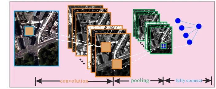
The CNN basically consists of three major operations: convolution, nonlinearity and 175

pooling/subsampling (Schmidhuber, 2015). The convolutional and pooling layers are 176

stacked together alternatively in the CNN framework, until obtaining the high-level 177

features on which a fully connected classification is performed (LeCun et al., 2015). In 178

addition, several feature maps may exist in each convolutional layer and the weights of 179

convolutional nodes in the same map are shared. This setting enables the network to 180

learn different features while keeping the number of parameters tractable. 181

Mathematically, the output feature map , ()

l j i

y at convolutional layer l is calculated as: 182



i w x b

y 1 1 ) ( ) 1 ( , ) ( , ) ( ) (

,  ( ) (4)

183

Where the , ()

l m n

w denotes the convolutional filter with size k×k at layer l, and the 184 ) 1 ( ,    l m j n i

x represents the spatial position of the corresponding feature map at the 185

preceding layer l-1. The algorithm passes the convolutional filter throughout the input 186

7

feature map using the dot product between them with an addition of a bias unit b(l)

187

(Arel et al., 2010). Moreover, a nonlinear activation function (l) at layer l is taken 188

outside the dot product to strengthen the nonlinearity (Strigl et al., 2010). 189

The pooling/subsampling layer can generalize the convolved features through down-190

sampling and thereby reduce the computational complexity during the training process 191

(Zhao and Du, 2016). Given a pooling/subsampling layer q, the feature output Fq can 192

be derived from the preceding layer f(q1) through 193

max( ,..., ,..., ,... ,1)

1 ), 1 ( 1 1 ) 1 ( 1 , 1 ) 1 ( 1 ), 1 ( 1 ,              q pj pi q pj i p q j p pi q j p i p q j

i f f f f

F

194

(5) 195

Where is the size of the local spatial region, and 1i,j(mn1)/p, here the 196

m refers to the size of input feature map, while n corresponds to the size of filter 197

(Längkvist et al., 2016). The simply summarizes the input features within local 198

spatial region using the maximum value (Figure 1: Pooling). By doing this, the learnt 199

features become robust and abstract with certain sparseness and translation invariance. 200

Once the higher level features are extracted, the output feature maps are flattened into 201

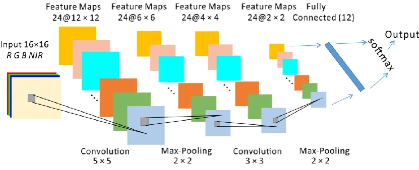
a one-dimensional vector, followed by a fully connected output layer (Figure 1: fully 202

connect). This operation is exactly a simple logistic regression, which is equivalent to 203

the standard MLP discussed in section 2.1, but without any hidden layer. 204

205

Figure 1 A schematic illustration of the three core layers within the CNN architecture, including the

206

convolutional layer (convolution), pooling layer (pooling) and fully connected layer (fully connect).

207

2.3 Hybrid MLP-CNN Classification Approach

8

Suppose the predictive outputs of the MLP and CNN at each pixel are n-dimensional 209

vectorsC(c1,c2,...,cn), where n represents the number of classes and each dimension 210

] , 1 [ n

i corresponds to the probability of a specific class (i-th class) with certain 211

membership association. Ideally, the probability of the classification prediction would 212

be 1 for the target class and 0 for the others. However, due to the uncertainty in the 213

process of remotely sensed image classification, the probability value c is denoted as 214

)} ,..., 2 , 1 ( | { )

(x c x n

f  x  , where cx[0,1] and



x

c

1 1 . The classification model

215

simply takes the maximum membership association as the predicted output label 216

(denoted as class(C)): 217

)}) ,..., 2 , 1 ( | ) ( max({ arg )

(C f x c x n

class   _x  (6)

218

The confidence conf of such membership association is defined here as: 219

) ( )

(C Mean C Max

conf   (7)

220

In equation (7), Max(C) represents the maximum value of vector C, while Mean(C) 221

denotes the average of all the values of C. The conf, quantified by the difference 222

between Max(C) and Mean(C), measures the confidence or reliability of the class 223

membership allocation (i.e. classification confidence map). Since the CNN takes 224

contextual image patches as its inputs instead of image pixels, it has the following 225

properties: 226

(1). If the input image patch is located at the central homogeneous region, its class 227

purity is relatively high with large difference between the membership association of 228

the predicted class and those of the other classes, and the conf tends to be large (White 229

regions in Figure 2(c)). 230

(2). If the image patch contains other land cover classes as contextual information, the 231

resulting distinction between the membership association of prediction and those of the 232

others is relatively low, and the conf tends to be small (Dark regions in Figure 2(c)). 233

However, the MLP (spectral feature only) is based on per-pixel spectral information, 234

thereby ruling out the difference of membership association between central and 235

9

aforementioned properties, the fusion decision rules are constructed primarily based on 237

CNN confidence. To be more specific, the fusion output gives credit to the CNN when 238

its confidence is larger than a predefined threshold (α1), while the MLP is trusted given 239

that the CNN confidence is lower than another threshold (α2); once the confidence of 240

the CNN lies in-between the two thresholds ((α₁,α₂)), the fusion output chooses the 241

CNN or MLP classification result with a larger confidence. Therefore, for a given image 242

pixel at location(h,v), a rule-based decision fusion approach to determining the class 243

label (class(h,v)) of the corresponding pixel is formulated as follows: 244                        2 2 1 2 1 1 ) & ( ) & ( ) , (       cnn mlp cnn cnn mlp cnn cnn cnn cnn cnn mlp mlp conf conf conf conf conf conf conf conf class class class class v h

class (8)

245

Where the class_mlp and class_cnn represent the classification results of the MLP and CNN 246

respectively; the conf_mlp and conf_cnn denote the classification confidence of the MLP 247

and CNN accordingly. 248

Estimation of the two thresholds (α1,α2) is conducted using grid search with cross-249

validation (Min and Lee, 2005; Zhang et al., 2015) based on the CNN classification 250

confidence map (as illustrated by Figure 2(c)). Specifically, the α1 was searched from 251

0.1 to 0.5 to detect those regions with low confidence as predicted by the CNN, while 252

the α2 was chosen from 0.5 to 0.9 to discover the high confidence regions. By initially 253

fixing α1 as 0.1, α2 was tuned with step size of 0.05 (i.e. α2=0.5, 0.55, 0.6, ..., 0.9) to 254

cross-validate the classification accuracy influenced by the selected thresholds; α1 was 255

then increased to further tune α2 in a similar way until the optimal α1 and α2 were found 256

with the best classification accuracy. 257

10

Figure 2 (a) A subset of the original imagery with RGB spectral bands, (b) the classification confidence

259

of the MLP and (c) the classification confidence of the CNN. The dark pixels represent low confidence,

260

while white pixels signify high confidence.

261

3. Experiment 262

3.1 Study area and data source

263

For this study, the city of Southampton, UK and its surrounding environment, which 264

lies on the south coast of England, was chosen as a case study area (Figure 3). The 265

urban and suburban areas in Southampton are strongly heterogeneous with a mixture of 266

anthropogenic urban surface (e.g. roof materials, asphalt, concrete) and semi-natural 267

environment (e.g. vegetation, bare soil), thereby representing a good test for 268

classification algorithms. 269

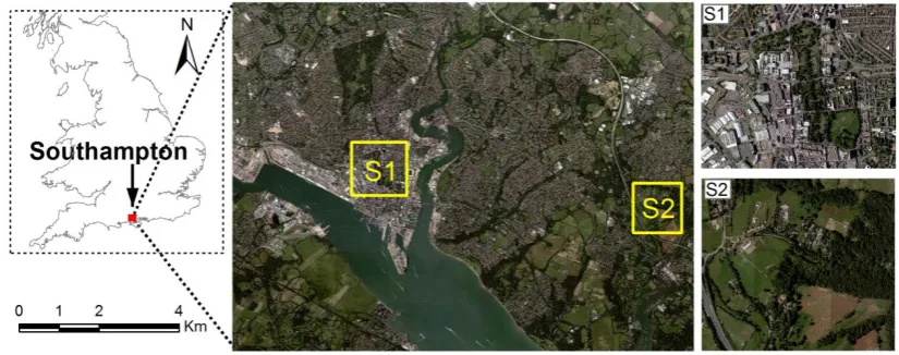
A scene of aerial imagery of Southampton was captured on 22 July 2012 using a Vexcel 270

UltraCam Xp digital aerial camera with 50 cm spatial resolution and four multispectral 271

bands (Red, Green, Blue and Near Infrared). Two study sites S1 (3087×2750 pixels) 272

and S2 (2022×1672 pixels) were selected to investigate the effectiveness of the 273

proposed algorithm. S1 is located in the city centre of Southampton, which consists of 274

eight dominant land cover classes, including Clay roof, Concrete roof, Metal roof, 275

Asphalt, Grassland, Trees, Bare soil and Shadow, with detailed descriptions listed in 276

Table 1. S2, on the other hand, is situated in a suburban and rural area of Southampton 277

comprised of large patches of forest, grassland and bare soil speckled with small 278

buildings and roads. There are six land cover categories in this study site, namely, 279

Buildings, Road-or-track, Grassland, Trees, Bare soil and Shadow (Table 1). 280

281

Figure 3 Southampton, UK Location of study area and aerial imagery with two study sites S1 and S2.

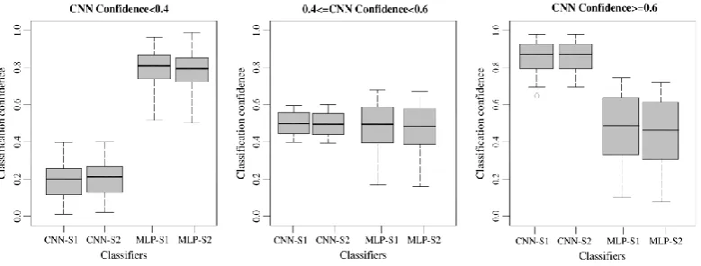
11

Sample points were collected using a stratified random scheme from ground data 283

provided by local surveyors at Southampton, and split into 50% training samples and 284

50% testing samples for each class (Table 1). Field land cover survey was conducted 285

throughout the study area on July 2012 to further check the validity and precision of 286

the selected samples. In addition, a highly detailed vector map from Ordnance Survey, 287

namely the MasterMap Topographic Layer (Regnauld and Mackaness, 2006), was fully 288

consulted and cross-referenced to gain a comprehensive appreciation of the land cover 289

and land use within the study area. 290

Table 1 Detailed description of land covers at two study sites with training and testing sample size per

291

class.

292

Study

Sites Class Train Test Description

S1

Clay roof 144 144 Predominantly residential buildings in red clay tiles

Concrete roof 132 132 Predominantly residential buildings in grey clay tiles

Metal roof 134 134 Predominantly industrial buildings in white metal panels

Asphalt 136 136 Urban road or cark parks covered by asphalt

Grassland 126 126 Areas of grass covering the urban park or lawn

Trees 137 137 Patches of tree species

Bare soil 118 118 Open areas covered by bare soil

Shadow 123 123 Areas of shadow cast from buildings and trees

S2

Building 82 82 Predominantly small buildings at rural areas

Road-or-track 85 85 Asphalt road or small path

Grassland 86 86 Large areas of wild grass or lawn

Trees 98 98 Large patches of deciduous trees

Bare soil 84 84 Open areas covered by bare soil

Shadow 86 86 Areas of shadow cast from buildings and trees

293

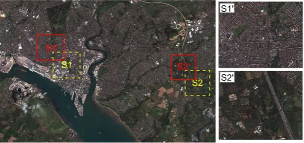
To further test the applicability of the proposed method, another scene of Worldview-294

2 satellite sensor imagery was acquired on 24 July 2013 in the same region of 295

Southampton with urban (S1’) and rural (S2’) study sites close to the Northwest of S1 296

and S2. The Worldview-2 image was geometrically and atmospherically corrected, and 297

pan-sharpened at 50 cm spatial resolution to be consistent with the aerial imagery. 298

Figure 4 demonstrates the WorldView-2 satellite sensor image together with two 299

12 301

Figure 4 Additional WorldView-2 satellite sensor image covering the same region of Southampton

302

with the S1’ and S2’ study sites to the northwest of S1 and S2, respectively.

303

3.2 Model input variables and parameters

304

Model inputs: the standard pixel-based MLP (hereafter, MLP) and CNN take only the 305

four spectral bands as their input variables, whereas the pixel-based texture MLP based 306

on the standard Grey Level Co-occurrence Matrix (hereafter, GLCM-MLP) 307

simultaneously makes use of both the four spectral bands and the texture features 308

derived from GLCM textural features including the Mean, Variance, Homogeneity, 309

Contrast, Dis-similarity, Entropy, Second moment and Correlation (Haralick et al., 310

1973; Rodriguez-Galiano et al., 2012; Xia et al., 2010; Zhang et al., 2003). Three 311

window sizes for each spectral band, including 3×3 (1.5×1.5 m), 5×5 (2.5×2.5 m), and 312

7×7 (3.5×3.5 m), were optimally chosen to perform multi-scale texture feature 313

representation, thus generating 96 GLCM texture features in total. It should be noted 314

that both the MLP and the CNN as well as the GLCM-MLP were trained to predict all 315

pixels within the images. Although the CNN was designed to predict a single label from 316

a small image patch, the sliding window was densely overlapping to cover the entire 317

image at the inference phase. 318

Both the MLP (also including GLCM-MLP) and CNN models require a series of 319

predefined parameters to optimize the learning accuracy and generalization capability. 320

Following the recommendations of Mas and Flores, (2008), the MLPs with one, two 321

and three hidden layers were tested, using a varying number of {4, 8, 12, 16, 20, and 322

24} nodes in each layer. The learning rate was chosen optimally as 0.2 and the 323

momentum factor was set as 0.7. In addition, the number of iterations was set as 1000 324

13

nodes and hidden layers, the best predicting MLP was found using two hidden layers 326

with 8 nodes in each layer. Similar parameters were also set for the GLCM-MLP, 327

except that two hidden layers with 20 nodes in each layer were found to be the optimal 328

solution in this case. 329

For the CNN, a range of parameters including the number of layers, the input image 330

patch size, the number and size of convolutional filter, as well as other predefined 331

parameters, such as the learning rate and number of epochs (iterations), need to be tuned 332

(Romero et al., 2016). Following the discussion by Längkvist et al., (2016), the input 333

image size was chosen from {8×8, 10×10, 12×12, 14×14, 16×16, 18×18, 20×20, 22×22 334

and 24×24} to evaluate the influence of context area on classification performance. In 335

general, a small-sized contextual area results in overfitting of the model, whereas a 336

large one often leads to under-segmentation. In consideration of the image object size 337

and contextual relationship coupled with a small amount of trial and error, the optimal 338

input image patch size was set to 16×16 in this research. Besides, as discussed by Chen 339

et al., (2014) and Längkvist et al., (2016), the depth plays a key role in classification 340

accuracy because the quality of learnt feature is highly influenced by the level of 341

abstraction and representation. As suggested by Chen et al. (2016), the number of CNN 342

layers was chosen as four to balance the network complexity and robustness. Other 343

parameters were set based on standard practice in the field of computer vision. For 344

example, the filter size was set to 5×5 for the first convolution layer and 3×3 for the 345

rest with stride of 1, and the number of the filters was set to 24 to extract multiple 346

convolutional features at each level. The fully connected layer was tuned as 12 nodes 347

followed by a softmax classification. The learning rate was set to 0.01 and the number 348

of epochs (iterations) was chosen as 600 to fully learn the features through 349

backpropagation. The detailed architecture of the CNN and its parameter configurations 350

14 352

Figure 5. The architecture of the CNN and its configurations.

353

3.3 Decision Fusion Parameter Setting and analysis

354

A rule-based decision fusion approach was implemented based on the classification 355

confidence maps of the CNN (e.g. Figure 2(b)) and MLP (e.g. Figure 2(c)). The 356

parameters of decision fusion, including two thresholds α1 and α2, were determined by 357

grid search with cross-validation using 10% of the randomly chosen samples. In this 358

study, the optimal thresholds α1=0.4 and α2=0.6 were found that reported the greatest 359

classification accuracy. 360

For the sake of visual interpretation, the confidence distribution of the CNN and MLP 361

influenced by the chosen thresholds is shown in Figure 6. Clearly, the CNN and MLP 362

demonstrated individually consistent, but mutually converse distribution patterns in the 363

two study sites: along with the increase in the CNN’s confidence, the MLP inversely 364

exhibited a decreasing trend. Specifically, for low CNN confidence (<0.4), the MLP 365

confidence was around 0.75, significantly higher than that of the CNN, thus outputting 366

the results of MLP in the final decision; once the CNN confidence ranged from 0.4 to 367

0.6, no significant difference was shown between the two classifiers, thereby, optimally 368

choosing the classification results based on the competitive “winner-takes-all” 369

approach; while for large CNN confidence (>0.6), the MLP was, in contrast, much less 370

15 372

Figure 6 Classification confidence distributions of the CNN and MLP at two study sites (S1 and S2)

373

under different fusion thresholds.

374

3.4 Classification results and analysis 375

3.4.1 Classification results and visual assessment

376

By integrating the classification results of the MLP and CNN using the above-377

mentioned fusion parameters, the final classification of the proposed MLP-CNN was 378

obtained at both study sites, S1 (city centre with complex urban scene) and S2 (rural 379

areas with natural phenomena). To provide a better visualization, Figure 7 (three 380

subsets of S1) and Figure 8 (three subsets of S2) highlights the correct or incorrect 381

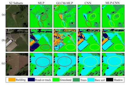
classification results of different classifiers marked in yellow or red circles, respectively. 382

From Figure 7, it can be seen that the MLP classification results consist of undesirable 383

noise (marked in red circle), such as a severe salt-and-pepper effect in Figure 7(a) and 384

7(b), and linear noisy textures in Figure 8(c). Besides, Trees and Grassland are seriously 385

confused with each other as illustrated by Figure 7(c) and Figure 8(a) and 8(b). 386

However, as shown by Figure 7(b), the MLP has certain advantages over CNN in 387

identifying the Clay roof class with spectrally distinctive features (marked in yellow 388

circle). With the addition of the GLCM textures, the GLCM-MLP achieved certain 389

improvements in both spectral and spatial pattern differentiation. For example, Trees 390

and Grassland are better distinguished to some extent compared with the pixel-based 391

MLP results, as illustrated in Figure 7(c) and Figure 8(b). Besides, the clear linear noisy 392

textures in Figure 8(c) are much reduced, and primarily turned into small speckles due 393

to the introduction of texture features. Yet, the GLCM-MLP falsely identifies some 394

16

(marked in red circle). Additionally, some geometrical distortions of building roof tops, 396

e.g. the Metal Roof and Concrete Roof in Figure 7(b), are shown in the GLCM-MLP 397

classification results caused by the GLCM texture filters. 398

In contrast to the pixel-based MLP and the GLCM-MLP, the classification results of 399

the CNN in both study sites exhibit smoothed visual effects with the least speckle noise 400

as shown by Figure 7 and 8. Additionally, the classes of green vegetation including 401

Grassland and Trees are accurately distinguished as demonstrated by the yellow circles 402

in Figure 7(c) and Figure 8(a) and 8(b) in spite of their spectral similarity. Moreover, 403

the CNN is able to discriminate the Concrete roof from Asphalt with a moderate 404

accuracy, as highlighted by the yellow circle in Figure 7(a). Nevertheless, the CNN 405

delivers some uncertainties in partitioning object boundaries. For example, the regular 406

shapes of some buildings (e.g. the geometries of some Clay roof and Concrete roof 407

areas) are distorted with false boundary partitions, as marked by the red circle in Figure 408

7(b). In addition, small or linear features are either merged into a large object or 409

discarded by over-smoothness. For instance, some Clay roof buildings (small objects) 410

are falsely connected together, while Asphalt is sometimes misclassified as Clay roof 411

(Figure 7(c)) and the small paths covered by Bare soil are discarded (Figure 8(b)). 412

With respect to the results of the MLP-CNN, all of the aforementioned 413

misclassifications produced by MLP or CNN are resolved with a higher resulting 414

accuracy. Thus, the incorrect classifications (marked by red circles) which appeared in 415

Figure 7 and 8 are revised accordingly, with no red circles appearing in the 416

classification results of MLP-CNN. The MLP-CNN modifies the classification errors 417

of the CNN for Asphalt, as illustrated by the red circles in Figure 7(c) and Figure 8(b), 418

thanks to the correct classification results of the MLP. Moreover, the linear-shaped Bare 419

Soil area missed by the CNN in Figure 8(a) is brought back correctly without losing 420

useful information. In addition, the original shapes of the Clay roof and Concrete roof 421

areas shown in Figure 7(b) are accurately restored. Most importantly, some mutual 422

misclassifications between the MLP and CNN are successfully rectified. For example, 423

the MLP-CNN correctly differentiates some Asphalt (with spectrally distinctive but 424

spatially confusing characteristics) and Concrete roof (distinctive in texture and 425

geometry but vague in spectrum) areas that are mutually misclassified by the MLP and 426

17 428

Figure 7 Three typical image subsets (a, b and c) in study site S1 with their classification results.

429

Columns from left to right represent the original images (R G B bands), the MLP classification, the

430

GLCM-MLP classification, the CNN classification and the MLP-CNN classification correspondingly.

431

The red and yellow circles denote incorrect and correct classification, respectively.

432

433

Figure 8 Three typical image subsets (a, b and c) in study site S2 with their classification results.

434

Columns from left to right represent the original images (R G B bands), the MLP classification, the

18

GLCM-MLP classification, the CNN classification and the MLP-CNN classification correspondingly.

436

The red and yellow circles denote incorrect and correct classification, respectively.

437

3.4.2Classification accuracy assessment

438

The classification performance of the proposed MLP-CNN approach was further 439

investigated through benchmark comparison with the MLP, GLCM-MLP and the CNN. 440

Table 2 lists the classification accuracy assessment, including the overall accuracy 441

(OA), Kappa coefficient (κ), and the class-wise mapping accuracy. From the table, it 442

can be seen that the decision fusion approach (MLP-CNN) consistently reports the best 443

classification OA with up to 90.93% for S1 and 89.64% for S2, higher than that of the 444

CNN (85.39% and 86.56%, respectively) and GLCM-MLP (83.12% and 82.63%, 445

respectively) as well as MLP (81.62% and 80.73%, respectively) (Table 2). Moreover, 446

a Kappa z-test for pair-wise comparison also shows that a significant increase in 447

classification accuracy has been achieved by the proposed MLP-CNN classifier over 448

the MLP, GLCM-MLP and CNN in S1, with z-value=3.68, 3.12 and 2.25, respectively. 449

For S2, the MLP-CNN also revealed a significant increase over the MLP with z -450

value=3.71 as well as GLCM-MLP with z-value=3.18, but no significant difference in 451

comparison with the CNN (z = 1.59, smaller than 1.96 at 95% confidence level) 452

(Congalton, 1991), despite the obvious improvement shown in Table 2. 453

The increase in classification accuracy was also checked by class-wise accuracy 454

assessment (Table 3). As illustrated by the table, MLP-CNN outperforms CNN for all 455

classes at both study sites in terms of classification accuracy. The largest increase is up 456

to 9.77% for the class of Concrete roof in S1 and 7.16% for the class of Road-or-track 457

in S2. Similar patterns were found such that the MLP-CNN was constantly superior to 458

GLCM-MLP at the class-wise level, where the greatest increase in accuracy was shown 459

up to 11.56% for the class of Concrete Roof in S1 and 11.74% for the class of Grassland 460

in S2. When compared with the MLP, most classes in the two sites except for Asphalt 461

and Shadow in S1 are classified with higher accuracy by the MLP-CNN. Here, 462

Grassland exhibits the highest increase in classification accuracy, up to 33.51% and 463

18.83% for S1 and S2, respectively. For the classes of Asphalt and Shadow, the 464

accuracy of the MLP is slightly larger than that of the MLP-CNN, but without a 465

19

With respect to the three benchmark classifiers themselves (i.e. MLP, GLCM-MLP and 467

CNN), it can be seen from Table 2 that their classification accuracies are ordered as: 468

MLP <GLCM-MLP < CNN. While the accuracy of CNN is remarkably higher (3%-469

5%) than that of the MLP and GLCM-MLP, the GLCM-MLP is just slightly higher 470

(<2%) than the MLP. The Kappa z-tests (Table 3) further demonstrate that the CNN is 471

statistically significantly more accurate than MLP and GLCM-MLP in both urban and 472

rural areas, whereas a significant increase in accuracy of the GLCM-MLP over the MLP 473

appears only in the rural area rather than the urban area. 474

Table 2 Classification accuracy comparison amongst MLP, GLCM-MLP, CNN and the proposed

MLP-475

CNN approach for study sites S1 and S2 using the per-class mapping accuracy, overall accuracy (OA)

476

and Kappa coefficient (κ). The bold font highlights the greatest classification accuracy per row.

477

Study

Sites Class MLP

GLCM-MLP

(Benchmark) CNN MLP-CNN

S1

Clay roof 92.26% 91.43% 90.11% 95.03%

Concrete roof 67.06% 62.44% 64.23% 74.00%

Metal roof 91.13% 90.36% 94.19% 94.63%

Asphalt 92.72% 88.67% 85.98% 91.26%

Grassland 60.51% 82.58% 90.73% 94.02%

Trees 63.88% 78.46% 82.28% 88.83%

Bare soil 79.63% 83.05% 86.16% 92.49%

Shadow 92.33% 91.06% 91.14% 91.52%

Overall Accuracy (OA) 81.62% 83.12% 85.39% 90.93%

Kappa Coefficient (κ) 0.78 0.81 0.84 0.89

S2

Building 82.83% 80.79% 83.08% 88.48%

Road or track 83.02% 80.14% 82.42% 89.58%

Grassland 71.11% 78.20% 88.34% 89.94%

Trees 79.31% 84.55% 90.70% 92.86%

Bare soil 74.07% 76.32% 81.36% 86.86%

Shadow 89.41% 88.25% 88.37% 90.17%

Overall Accuracy (OA) 80.73% 82.63% 86.56% 89.64%

Kappa Coefficient (κ) 0.78 0.79 0.84 0.87

478

Table 3 Kappa z-test (p-value) comparing the performance of the three classifiers for two study sites S1

479

and S2. Significantly different accuracies with confidence of 95% (z-value > 1.96 with p-value < 0.05)

480

are indicated by *.

20

Study sites Classifiers

Kappa Z-test (p-value)

MLP GLCM-MLP

(Benchmark) CNN

MLP-CNN

S1

MLP —

GLCM-MLP 1.56 (0.1188) —

CNN 2.64* (0.0083) 2.44* (0.0147) —

MLP-CNN 3.68* (0.0002) 3.12* (0.0018) 2.25* (0.0244) —

S2

MLP —

GLCM-MLP 2.05* (0.0404) —

CNN 2.51* (0.0121) 2.36* (0.0183) —

MLP-CNN 3.71* (0.0002) 3.18* (0.0015) 1.59 (0.1118) —

482

The proposed MLP-CNN method and the other three benchmarks (MLP, GLCM-MLP 483

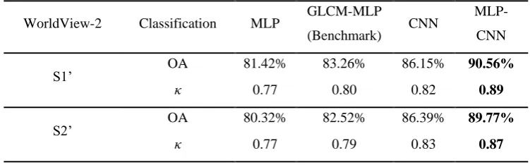
and the CNN) were also validated using an additional WorldView-2 satellite sensor 484

dataset at the S1’ and S2’ study sites. The OA and κ of both study sites are in accordance 485

with the results of aerial photo classification, where the decision fusion approach (MLP-486

CNN) acquires the largest OA of 90.56% at S1’ and 89.77% at S2’, consistently higher 487

than the CNN (86.15% and 86.39%), the GLCM-MLP (83.26% and 82.52%) and the 488

MLP (81.42% and 80.32%) (Table 4). Such coherency of classification results further 489

demonstrates the wide applicability of the proposed method with different datasets. 490

Table 4 Classification accuracy comparison amongst MLP, GLCM-MLP (Benchmark), CNN and the

491

proposed MLP-CNN approach for study sites S1’ and S2’ from the WorldView-2 satellite sensor image

492

using overall accuracy (OA) and Kappa coefficient (κ). The bold font highlights the greatest

493

classification accuracy per row.

494

WorldView-2 Classification MLP GLCM-MLP

(Benchmark) CNN

MLP-CNN

S1’ OA 81.42% 83.26% 86.15% 90.56%

κ 0.77 0.80 0.82 0.89

S2’ OA 80.32% 82.52% 86.39% 89.77%

κ 0.77 0.79 0.83 0.87

495

21

In this research, a rule-based decision fusion approach (MLP-CNN) was proposed to 497

integrate classifiers of the pixel-based MLP with shallow structures and the contextual-498

based CNN with deep architectures for the classification of VFSR remotely sensed 499

imagery. The MLP-CNN takes advantage of the merits of the two classifiers and 500

overcomes their individual shortcomings as discussed below. 501

4.1 Characteristics of MLP and GLCM-MLP classification

502

In principle, the MLP builds the decision boundaries among classes in feature space 503

based on per-pixel spectral information (Mokhtarzade and Zoej, 2007). Such 504

classification boundaries are very sensitive to the class with salient spectral properties 505

that are spectrally distinctive from other classes (Berberoglu et al., 2000). For example, 506

classes like Clay roof, Asphalt and Shadow in Site 1 are spectrally exclusive to other 507

classes, leading to high classification accuracies, up to 92.26%, 92.72% and 92.33%, 508

respectively (Table 2). However, the MLP relies on the pixel-based spectral information 509

in the classification process without exploiting the abundant spatial information 510

appearing in the VFSR imagery (e.g. texture, geometry or contextual relationship) 511

(Wang et al., 2016). These limitations often result in unsatisfactory classification 512

performance; for example, confusion and misclassification between the Trees and 513

Grassland classes that are spectrally similar. Even for those correctly identified objects, 514

severe salt and pepper effects still exist (Dark and Bram, 2007), for example, the linear 515

texture noise appearing for Bare soil in Figure 8(c). For these reasons, the classification 516

accuracy of MLP is generally statistically significantly lower than that of the CNN and 517

the proposed MLP-CNN. However, objects in VFSR imagery are mostly depicted by 518

pure pixels, especially for human-made features with crisp boundaries, such as 519

buildings, residential houses and cultivated land. The membership association of a pixel 520

deduced by MLP is, therefore, not affected by its relative position (e.g. lying on or close 521

to boundaries), as long as the corresponding spectral space is separable. 522

The inclusion of GLCM texture features in the GLCM-MLP classifier enables the 523

model to process spectral and spatial information simultaneously. Those GLCM texture 524

descriptors are handcrafted features that are designed to capture statistical co-525

occurrence information (Xia et al., 2010). However, the GLCM textures are essentially 526

first or second order feature transformations instead of feature learning. Such hand-527

22

challenging to generalize to other domains and datasets. Besides, the addition of 96 529

GLCM textures results in a dramatically increased number of input variables, which 530

leads to a relatively high dimensional feature space. The so-called “curse of 531

dimensionality” (Hughes, 1968) and collinearity make the GLCM-MLP hard to 532

parameterize and potentially leads to texture overfitting. That is why the GLCM-MLP 533

cannot substantially increase the classification accuracy compared to the MLP. That is, 534

the spectral and spatial information cannot be effectively exploited by the GLCM-MLP. 535

For example, some spectrally different classes but with similar textures such as Clay 536

Roof, Concrete Roof and Asphalt are confused to some degree. 537

4.2 Characteristics of CNN classification

538

Spatial features in remotely sensed data like VFSR imagery are intrinsically local 539

(especially in lower layers) and spatially invariant (Masi et al., 2016). The MLP, 540

however, assumes that the location of the data in the input is irrelevant to the model 541

construction and it is, thus, incapable of learning spatial features of remote sensing data. 542

In contrast, by using multiple convolution and pooling operations, CNN models the 543

way that the human visual cortex works and enforces weight sharing with translation 544

invariance that enables the extraction of high-level spatial features from image patches. 545

It should be mentioned that the pooling operations play an important role in dimension 546

reduction, thus, avoiding “the curse of dimensionality” present in the GLCM-MLP 547

classifier. Thanks to these superior characteristics, the CNN classifier outperforms the 548

MLP and GLCM-MLP classifiers in both the urban scene and rural areas. Especially, 549

classes like Concrete roof and Road-or-track that are difficult to distinguish from their 550

backgrounds with only spectral or low-level features (e.g. distance between the 551

prediction and the target class at spectral space), are identified with relatively high 552

accuracies. In addition, classes with heavy spectral confusion in both study sites (e.g. 553

Trees and Grassland), are accurately differentiated due to their obvious spatial pattern 554

differences; for example, the texture of tree canopies is generally much rougher than 555

for grassland. As a contextual classifier with deep architectures, the CNN could reveal 556

the spatial patterns hidden in the image data that cannot be perceived by its shallow 557

counterparts (e.g. MLP classifier or even the GLCM-MLP classifier). The higher layers 558

in CNN models provide more semantically meaningful information concentrating on 559

global semantics rather than local or pixel-level information, making the CNN 560

23

Yang et al., 2015). Therefore, the CNN shows an impressive stability and effectiveness 562

in spatial feature representation, which is crucial for VFSR image classification (Zhao 563

and Du, 2016). 564

However, according to the “no free lunch” theorem (Wolpert and Macready, 1997), any 565

elevated performance in one aspect of a problem will be paid for through others, and 566

the CNN is no exception. Using contextual image patches as inputs and learning deep 567

spatial features, the CNN demonstrates power in spatial pattern recognition but also 568

weakness in spatial partition. Boundary uncertainties (over-smoothness) often appear 569

in the classified object and small useful features are erased, somewhat similar to 570

morphological or Gabor filter methods (Pingel et al., 2013; Reis and Tasdemir, 2011). 571

For example, the human-made objects in urban scenes like buildings and asphalt are 572

often geometrically enlarged with distortion to some degree (See Figure 7(b)). As for 573

natural objects in rural areas (S2), edges or porosities of a landscape patch are simplified 574

or ignored, and even worse, linear features like river channels or dams that are of 575

ecological importance, are erroneously erased. One may argue that the reduction of 576

image patch size might be able to detect small features by multiple CNNs by varying 577

the contextual filter size as adopted in Längkvist et al. (2016). However, objects, 578

whether large or small in size, all have boundaries, thus, retaining the problem of 579

smoothing edges. In addition, the adoption of convolution and pooling operations 580

intrinsically reduces the image contextual size but strengthens the spatial feature 581

representation. Thus, a far too small initial image patch size can limit the network depth 582

of a CNN model. In fact, the currently used 16×16 window size is close to the minimum 583

requirements for a deep CNN with four hidden layers in total. Moreover, certain 584

spectrally distinctive features without obvious spatial patterns are poorly differentiated. 585

For example, some Asphalt pixels are wrongly identified as Concrete roofs as illustrated 586

in Figure 7(a). This further demonstrates the necessity of introducing spectral features 587

for VFSR image classification. 588

4.3 fusion decision of MLP-CNN classification

589

Huge uncertainty and inconsistency exists inherently in any remotely sensed data 590

(including VFSR imagery), and this runs through the training and the testing samples. 591

In fact, different classification algorithms vary in terms of remote sensing data 592

24

2015) to various applications of VFSR image classification, even for the powerful CNN 594

classifier with deep spatial feature representations. It is therefore especially important 595

to make use of the complementarities of different classifiers. It should be mentioned 596

that, the more heterogeneous the classification algorithms’ behaviours, the more that 597

different places might be accurately classified by each individual classifier, and the 598

more accurate the ensemble classifier might be (Löw et al., 2015). An ideal ensemble 599

classifier, thereby, should be established using individual classifiers that are very 600

differently behaved. 601

The experimental results show that the pixel-based MLP classifier with shallow 602

structures and the contextual-based CNN classifier with deep architectures can provide 603

complementary information, leading to a more accurate classification result than either 604

classifier alone. In addition to the elimination of heavy noise, the CNN can accurately 605

identify classes with rich spatial information implicit in VFSR data. Such 606

characteristics of the CNN emphasize the limitations of the MLP classifier for VFSR 607

image classification. At the same time, the CNN might lose some useful details, and it 608

has difficulties in utilizing spectral information and delineating object boundaries and 609

is, thus, incapable of maintaining geometric fidelity. The MLP classifier, however, 610

compensates directly with regard to the limitations of the CNN. The aforementioned 611

complementary properties between the CNN and MLP are well reflected from the 612

inverse confidence trends of the two classifiers (Figure 2). Specifically, in the case of 613

the CNN with the highest confidence, the MLP has the least confidence and vice versa, 614

which further indicates that the proposed MLP-CNN ensemble classifier can take 615

advantage of the MLP and CNN. 616

The proposed fusion decision rules were derived primarily on the basis of the CNN’s 617

confidence distribution, in consideration of the superiority of CNN classification 618

performance and the regularity of its confidence distribution. Such a decision fusion 619

strategy captures the patterns of the complementarities between the two individual 620

classifiers in general, thus, achieving a desirable classification result. At the same time, 621

the MLP-CNN classifier demonstrates great utility and wide applicability for both 622

aerial photography and WorldView-2 satellite sensor imagery with consistent and 623

competitive classification performance. However, in comparison with MLP, the 624

classification accuracies of Asphalt and Shadow were slightly higher than for the 625

25

decision fusion rules at the class-wise level for VFSR image classification. It might be 627

better to incorporate the spectral separability differentiated by MLP to achieve the best 628

classification performance at class level. Besides, no significant improvement was 629

acquired for rural areas (S2) by the MLP-CNN compared with the CNN. This is mainly 630

due to the ineffectiveness of the MLP in classifying natural features that dominate in 631

the rural environment. This shortcoming might be overcome by the replacement of the 632

MLP by other non-parametric machine learning classifiers (e.g. SVM, RF, etc.). 633

Moreover, incorporating other data sources (e.g. digital surface model) might be needed 634

to increase the accuracy of the MLP-CNN for both the CNN and MLP with very low 635

confidence simultaneously. These aforementioned issues will be investigated in future 636

research. 637

5. Conclusion 638

Due to its high intra-class variability and low inter-class disparity, VFSR image 639

classification poses great challenges to any single machine learning algorithm, even for 640

the powerful deep learning convolutional neural network (CNN). In this paper, two 641

neural network classifiers with strong heterogeneous behaviours (i.e. pixel-based MLP 642

with shallow structures and contextual-based CNN with deep architectures), were 643

integrated in a concise and effective way using a rule-based decision fusion strategy. 644

The decision fusion rules, designed primarily on the basis of the classification 645

confidence of the CNN, reflect the general complementary patterns of both the MLP 646

and CNN. In consequence, the proposed ensemble classifier MLP-CNN harvests the 647

complementary results acquired from the CNN with deep spatial feature representations 648

(CNN) and from the MLP based on spectral discrimination. Meanwhile, limitations of 649

the CNN such as uncertainty in object boundary partition and loss of useful fine 650

resolution detail were compensated. The effectiveness of the new MLP-CNN algorithm 651

was tested in both urban and rural areas using aerial and satellite sensor images. The 652

MLP-CNN algorithm consistently outperformed both of the individual classifiers (MLP 653

and CNN) as well as the GLCM-MLP that includes the GLCM texture features, with a 654

statistically significant difference in the majority of cases. This research paves the way 655

to an effective solution to the complicated problem of automatic VFSR image 656

classification. 657

26

This research was funded by PhD studentship “Deep Learning in massive area, multi-659

scale resolution remotely sensed imagery” (NO. EAA7369), sponsored by Ordnance 660

Survey and Lancaster University. The authors thank to the staff from the Ordnance 661

Survey for the supply of aerial imagery and supporting ground data. The authors also 662

thank to the two anonymous referees for their constructive comments on this 663

manuscript. 664

Reference 665

Ardila, J.P., Tolpekin, V.A., Bijker, W., Stein, A., 2011. Markov-random-field-based 666

super-resolution mapping for identification of urban trees in VHR images. 667

ISPRS J. Photogramm. Remote Sens. 66, 762–775. 668

doi:10.1016/j.isprsjprs.2011.08.002 669

Arel, I., Rose, D.C., Karnowski, T.P., 2010. Deep machine learning - A new frontier 670

in artificial intelligence research. IEEE Comput. Intell. Mag. 5, 13–18. 671

doi:10.1109/MCI.2010.938364 672

Atkinson, P.M., Tatnall, A.R.L., 1997. Introduction Neural networks in remote 673

sensing. Int. J. Remote Sens. 18, 699–709. doi:10.1080/014311697218700 674

Attarchi, S., Gloaguen, R., 2014. Classifying complex mountainous forests with L-675

Band SAR and landsat data integration: A comparison among different machine 676

learning methods in the Hyrcanian forest. Remote Sens. 6, 3624–3647. 677

doi:10.3390/rs6053624 678

Benediktsson, J.A., 2009. Ensemble classification algorithm for hyperspectral remote 679

sensing data. IEEE Geosci. Remote Sens. Lett. 6, 762–766. 680

doi:10.1109/LGRS.2009.2024624 681

Berberoglu, S., Lloyd, C.D., Atkinson, P.M., Curran, P.J., 2000. The integration of 682

spectral and textural information using neural networks for land cover mapping 683

in the Mediterranean. Comput. Geosci. 26, 385–396. doi:10.1016/S0098-684

3004(99)00119-3 685

Bezak, P., Bozek, P., Nikitin, Y., 2014. Advanced robotic grasping system using deep 686

learning. Procedia Eng. 96, 10–20. 687

27

Breiman, L., 1996. Bagging Predictors. Mach. Learn. 24, 123–140. 689

Chen, S., Member, S., Wang, H., Xu, F., Member, S., 2016. Target classification 690

using the deep Convolutional Networks for SAR images. IEEE Trans. Geosci. 691

Remote Sens. 54, 4806–4817. 692

Chen, Y., Jiang, H., Li, C., Jia, X., Member, S., 2016. Deep feature extraction and 693

classification of hyperspectral images based on Convolutional Neural Networks. 694

IEE Trans. Geosci. Remote Sens. 54, 6232–6251. 695

doi:10.1109/TGRS.2016.2584107 696

Chen, Y., Lin, Z., Zhao, X., Wang, G., Gu, Y., 2014. Deep learning-based 697

classification of hyperspectral data. IEEE J. Sel. Top. Appl. Earth Obs. Remote 698

Sens. 7, 2094–2107. doi:10.1109/JSTARS.2014.2329330 699

Clinton, N., Yu, L., Gong, P., 2015. Geographic stacking: Decision fusion to increase 700

global land cover map accuracy. ISPRS J. Photogramm. Remote Sens. 103, 57– 701

65. doi:10.1016/j.isprsjprs.2015.02.010 702

Congalton, R.G., 1991. A review of assessing the accuracy of classifications of 703

remotely sensed data. Remote Sens. Environ. 37, 35–46. 704

Dark, S.J., Bram, D., 2007. The modifiable areal unit problem (MAUP) in physical 705

geography. Prog. Phys. Geogr. 31, 471–479. doi:10.1177/0309133307083294 706

Del Frate, F., Pacifici, F., Schiavon, G., Solimini, C., 2007. Use of neural networks 707

for automatic classification from high-resolution images. IEEE Trans. Geosci. 708

Remote Sens. 45, 800–809. doi:10.1109/TGRS.2007.892009 709

Demarchi, L., Canters, F., Cariou, C., Licciardi, G., Chan, J.C.W., 2014. Assessing 710

the performance of two unsupervised dimensionality reduction techniques on 711

hyperspectral APEX data for high resolution urban land-cover mapping. ISPRS 712

J. Photogramm. Remote Sens. 87, 166–179. doi:10.1016/j.isprsjprs.2013.10.012 713

Dong, Z., Pei, M., He, Y., Liu, T., Dong, Y., Jia, Y., 2015. Vehicle type classification 714

using unsupervised Convolutional Neural Network. IEEE Trans. Intell. Transp. 715

Syst. 16, 2247–2256. doi:10.1109/ICPR.2014.39 716

28

for remote sensing image classification: A review. Sensors 12, 4764–4792. 718

doi:10.3390/s120404764 719

Farabet, C., Couprie, C., Najman, L., Lecun, Y., 2013. Learning hierarchical features 720

for scene labeling. IEEE Trans. Pattern Anal. Mach. Intell. 35, 1915–1929. 721

doi:10.1109/TPAMI.2012.231 722

Fauvel, M., Chanussot, J., Benediktsson, J.A., 2012. A spatial-spectral kernel-based 723

approach for the classification of remote-sensing images. Pattern Recognit. 45, 724

381–392. doi:10.1016/j.patcog.2011.03.035 725

Fauvel, M., Chanussot, J., Benediktsson, J.A., 2006. Decision fusion for the 726

classification of urban remote sensing images. IEEE Trans. Geosci. Remote 727

Sens. 44, 2828–2838. doi:10.1109/TGRS.2006.876708 728

Foody, G.M., Arora, M.K., 1997. An evaluation of some factors affecting the 729

accuracy of classification by an artificial neural network. Int. J. Remote Sens. 18, 730

799–810. doi:10.1080/014311697218764 731

Freund, Y., Iyer, R., Schapire, R.E., Singer, Y., 2003. An efficient boosting algorithm 732

for combining preferences. J. Mach. Learn. Res. 4, 933–969. 733

Haralick, R.M., Shanmugam, K., Dinstein, I., 1973. Textural Features for Image 734

Classification. IEEE Trans. Syst. Man. Cybern. 3, 610–621. 735

doi:10.1109/TSMC.1973.4309314 736

Hu, F., Xia, G.-S., Hu, J., Zhang, L., 2015a. Transferring Deep Convolutional Neural 737

Networks for the Scene Classification of High-Resolution Remote Sensing 738

Imagery. Remote Sens. 7, 14680–14707. doi:10.3390/rs71114680 739

Hu, F., Xia, G.S., Wang, Z., Huang, X., Zhang, L., Sun, H., 2015b. Unsupervised 740

Feature Learning Via Spectral Clustering of Multidimensional Patches for 741

Remotely Sensed Scene Classification. IEEE J. Sel. Top. Appl. Earth Obs. 742

Remote Sens. 8, 2015–2030. doi:10.1109/JSTARS.2015.2444405 743

Huang, X., Lu, Q., Zhang, L., 2014. A multi-index learning approach for 744

classification of high-resolution remotely sensed images over urban areas. ISPRS 745