Statistical Delay QoS Driven
Resource Allocation and Performance Analysis
for Wireless Communication Networks
Wenjuan Yu
School of Computing and Communications
Lancaster University
A thesis submitted for the degree of
Doctor of Philosophy
Abstract
Delay quality-of-service (QoS) guarantees play a critical role in enabling delay-sensitive wireless applications. By applying the theory of effective capacity (EC), the maximum arrival rate with a guaranteed delay-outage probability constraint, is analyzed and investigated in terms of delay-constrained resource allocation and link-layer throughput analysis.
Firstly, a joint optimization problem of link-layer energy efficiency (EE) and EC in a single-user single-carrier communication system, is proposed and investigated, under a delay violation probability requirement and an average transmit power constraint. Formulated as a normalized multi-objective optimization problem (MOP), the problem is transformed into a weighted single-objective optimization problem (SOP), and then solved. The proposed optimal power value is proved to be sufficient for the Pareto optimal set of the original EE-EC MOP.
Secondly, a total EC maximization problem subject to the individual link-layer EE requirement as well as the per-user average transmit power limit, in a multi-user multi-carrier orthogonal frequency-division multiple access (OFDMA) system, is proposed and analyzed. Formulated as a combina-torial integer programming problem, the problem is decoupled into a fre-quency provisioning problem and an independent per-user multi-carrier EE-EC tradeoff problem. A low-complexity heuristic algorithm is pro-posed to obtain the subcarrier assignment solution coupled with a per-user optimal power allocation strategy, across frequency and time domains.
Acknowledgements
First of all, I would like to express my sincere gratitude to my supervisors, Prof. Qiang Ni and Dr. Leila Musavian, for their patient guidance and continuous support, during the past four years of my Ph.D. study. Their commitment to solid and high-quality research work impressed me most and will keep me motivated in the future.
My sincere appreciation also goes to all academic and administrative staff in the School of Computing and Communications, for their professional advice, valuable support, and interesting seminars held regularly. It has been my pleasure to work with everyone of you in such a warm group.
List of Publications
Journal papers
1. W. Yu, L. Musavian and Q. Ni, ”Tradeoff Analysis and Joint Op-timization of Link-Layer Energy Efficiency and Effective Capacity Toward Green Communications”, IEEE Trans. Wireless Commun., vol. 15, no. 5, pp. 3339-3353, Jan. 2016.
2. W. Yu, L. Musavian and Q. Ni, ”Statistical Delay QoS Driven En-ergy Efficiency and Effective Capacity Tradeoff for Uplink Multi-User Multi-Carrier Systems”, IEEE Trans. Commun., vol. 65, no. 8, pp. 3494-3508, Apr. 2017.
3. W. Yu, L. Musavian and Q. Ni, ”Link-Layer Capacity of NOMA Under Statistical Delay QoS Guarantees”, submitted to IEEE Trans. Commun.
Conference papers
1. W. Yu, L. Musavian and Q. Ni, ”Weighted Tradeoff between Effec-tive Capacity and Energy Efficiency”, in IEEE Int. Conf. Commun. (ICC), London, UK, Jun. 2015, pp. 238-243.
2. W. Yu, L. Musavian and Q. Ni, ”Multi-carrier Link-Layer Energy Efficiency and Effective Capacity Tradeoff”, in IEEE Int. Conf. Commun. (ICC) Workshop, London, UK, Jun. 2015, pp. 2763-2768.
Contents
Abstract ii
Acknowledgements iii
List of Publications iv
List of Tables ix
List of Figures x
List of Acronyms xiii
List of Symbols and Mathematical Operators xv
1 Introduction 1
1.1 Motivations . . . 1
1.2 Thesis Outline and Contributions . . . 3
1.2.1 Thesis Contributions . . . 3
1.2.2 Thesis Outline . . . 7
2 Background Theory and Literature Review 8 2.1 The Theory of Effective Capacity . . . 8
2.1.1 Large Deviation Theory . . . 8
2.1.2 Envelope Process . . . 13
2.1.2.1 Deterministic Envelope Process . . . 13
2.1.2.2 Statistical Envelope Process . . . 14
2.1.3 Effective Bandwidth . . . 15
2.1.4 Effective Capacity . . . 17
2.2 Convex Optimization Theory . . . 20
2.2.2 Lagrangian Dual and KKT Conditions . . . 21
2.3 Literature Review . . . 22
2.3.1 Resource Allocation Towards Green Communications . . . 22
2.3.2 Current Research Progress in NOMA Networks . . . 27
3 Single-User Single-Carrier Link-Layer EE-EC Tradeoff 29 3.1 Introduction . . . 29
3.2 System Model and Problem Formulation . . . 30
3.2.1 System Model . . . 30
3.2.2 Problem Formulation . . . 31
3.3 Link-layer EE-EC tradeoff . . . 33
3.3.1 Effective Capacity and Link-layer Energy Efficiency . . . 33
3.3.2 Optimal Power Allocation . . . 34
3.3.2.1 Optimum Power Allocation with No Input Power Con-straint . . . 35
3.3.2.2 Optimal Power Allocation under Average Input Power Constraint . . . 39
3.3.3 The Impact of w1, Pnorm, Pcr and ǫ on the EE-EC Tradeoff . . 41
3.4 Numerical Results . . . 42
3.5 Summary . . . 53
4 Multi-User Multi-Carrier Link-Layer EE-EC Tradeoff 54 4.1 Introduction . . . 54
4.2 System Model and Problem Formulation . . . 55
4.2.1 System Model . . . 55
4.2.2 Effective Capacity and Link-Layer Energy Efficiency . . . 57
4.2.3 Problem Formulation . . . 59
4.3 Optimal and Sub-optimal Solutions . . . 60
4.3.1 Frequency Provisioning Algorithms . . . 61
4.3.1.1 Traditional Exhaustive Algorithm . . . 61
4.3.1.2 Fair-Exhaustive Algorithm . . . 62
4.3.1.3 Heuristic Algorithm . . . 63
4.3.2 Optimal Power Allocation for a Single-User Multi-Carrier System 65 4.3.2.1 Case 1 :Pr k,n>0,∀ n∈ Nk . . . 68
4.3.2.2 Case 2 :Pr k,j = 0, ∃ j ∈ Nk . . . 68
4.3.3 The Impact of Pk
4.4 Simulation Results . . . 72
4.5 Summary . . . 82
5 Link-Layer Rate in a Downlink NOMA Network 84 5.1 Introduction . . . 84
5.2 System Model . . . 85
5.3 Effective Capacity . . . 86
5.4 Effective Capacity in a Downlink NOMA Network . . . 87
5.4.1 Effective Capacity in a Two-user NOMA Network . . . 88
5.4.1.1 The Closed-Form Expressions for the Individual EC in a Two-user System . . . 89
5.4.1.2 Case 1: Consider Delay-Constrained Users . . . 92
5.4.1.3 Case 2: Consider Delay-Unconstrained Users . . . 96
5.4.2 Effective Capacity of Multiple NOMA Pairs . . . 97
5.5 Numerical Results . . . 99
5.6 Summary . . . 107
6 Conclusions and Future Work 108 6.1 Summary . . . 108
6.2 Future Work . . . 112
Appendix A Proof of Lemma 1 114
Appendix B Proof of Theorem 5 115
Appendix C Proof of Theorem 6 116
Appendix D Proof of Lemma 2 118
Appendix E Proof of Lemma 3 119
Appendix F Proof of Lemma 4 123
Appendix G Proof of Lemma 6 125
Appendix H Proof of Theorem 7 127
Appendix I Proof of Lemma 8 130
Appendix K Proof of Lemma 10 134
Appendix L Proof of Lemma 11 135
Appendix M Proof of Lemma 12 136
Appendix N Proof of Lemma 13 137
List of Tables
3.1 Optimal Power Allocation Algorithm for a Single-User Single-Carrier System . . . 40
4.1 Heuristic Algorithm for a Multi-User Multi-Carrier System . . . 64 4.2 Optimal Power Allocation Algorithm for a Single-User Multi-Carrier
List of Figures
2.1 EC and EB, as functions of the delay QoS exponent θ. . . 19
3.1 Block diagram for a point-to-point wireless communication link. . . . 31 3.2 EC and link-layer EE versus importance weight w1 for various values
of Pcr in Rayleigh fading channels. . . 44 3.3 EC versus scaled average input power limit Pmax
Kℓ
for various values of importance weight w1 in Rayleigh fading channels. . . 45
3.4 Maximum achievable EE versus scaled average power limit Pmax Kℓ
for various values of w1 in Rayleigh fading channels. . . 45
3.5 Normalized optimum average power valueP∗
r versus importance weight
w1 for various values of fading parameter m. . . 46
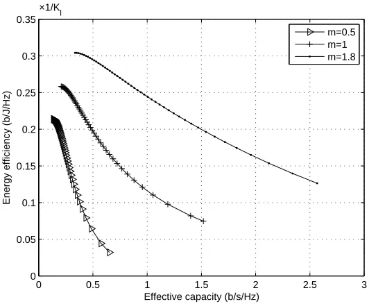
3.6 Maximum achievable EE versus EC for various values of Nakagami fading parameter m. . . 47 3.7 Maximum achievable EE versus importance weight w1 for various
val-ues of Pnorm in Rayleigh fading channels. . . 47
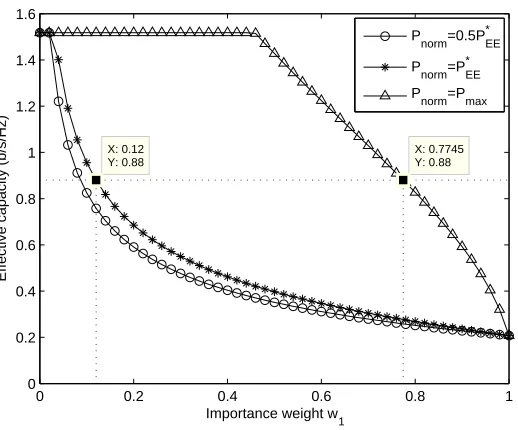
3.8 EC versus importance weight w1 for various values of normalization
factor Pnorm in Rayleigh fading channels. . . 48
3.9 EC and link-layer EE versus importance weight w1 for various values
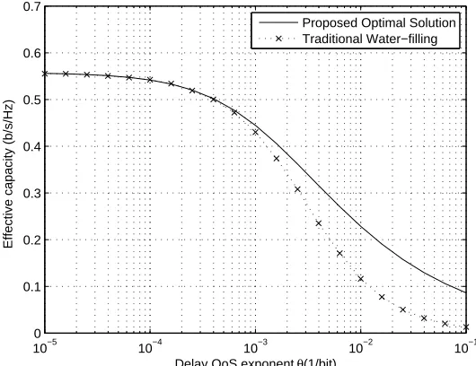
of θ in Rayleigh fading channels. . . 49 3.10 EC versus delay QoS exponentθ under different power allocation
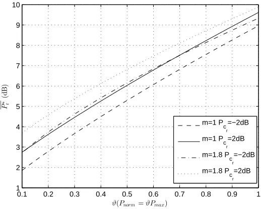
poli-cies in Rayleigh fading channels. . . 49 3.11 Normalized optimum average power value P∗
r versusϑ for various
val-ues of fading parameter m and scaled circuit-to-noise power ratio Pcr. 50 3.12 Maximum achievable EE versusϑfor various values of Nakagami fading
parameter m and scaled circuit-to-noise power ratio Pcr. . . 51 3.13 Normalized optimum average power valueP∗
r versusθfor various values
3.14 Delay-outage probability versus θ for various values ofw1 and
normal-ization factor Pnorm in Rayleigh fading channels. . . 52
4.1 Uplink transmission in a multi-user multi-carrier network. . . 56 4.2 Queuing system model for each transmitter. . . 57 4.3 Transform ηk
req toSreqk . . . 62
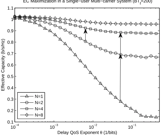
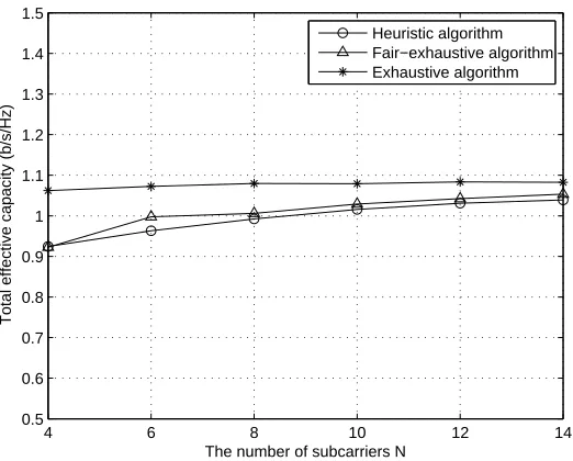
4.4 Effective capacity versus delay QoS exponent θ, for various values ofN. 65 4.5 The total effective capacity versus the number of subcarriers N, for
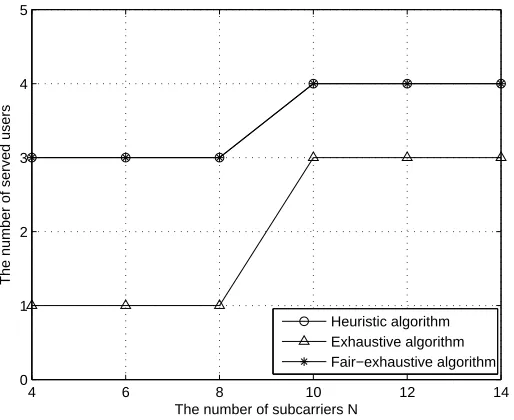
heuristic algorithm, exhaustive algorithm and fair-exhaustive algorithm. 72 4.6 The number of served users versus the number of subcarriers N, for
heuristic algorithm, exhaustive algorithm and fair-exhaustive algorithm. 73 4.7 The optimal average tradeoff power value versus delay QoS exponent
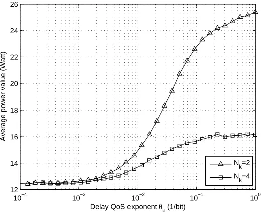
θk, for various values of Nk. . . 74
4.8 Effective capacity versus delay QoS exponent θk, for various values of
Nk. . . 75
4.9 The total effective capacity versus the number of usersK, for heuristic algorithm and exhaustive algorithm. . . 76 4.10 The total effective capacity versus the number of users K1 in group
K1, for various values of Pcr. . . 77 4.11 Link-layer energy efficiency and the optimal average power versus
circuit-to-noise power ratio Pk
cr, for various values of χ
k
EE. . . 78
4.12 Effective capacity and link-layer energy efficiency versus χk
EE, for
vari-ous values of θk and Nk. . . 79
4.13 The total effective capacity versus EE requirement factor for differ-ent values of delay QoS expondiffer-ent in heuristic algorithm, and fair-exhaustive algorithm. . . 80 4.14 The total effective capacity versus maximum power value, for different
values of θ. . . 81 4.15 Delay-outage probability versus delay QoS exponent θk, for different
values of χEE. . . 82
5.1 Two-user downlink NOMA network. . . 88 5.2 Em
c and Ecn, in NOMA, versus ρ for various values of the delay QoS
exponent vector θ. . . 100 5.3 Em
c , in NOMA, and ¯Ecm, in OMA, versus the transmit SNR ρ for
5.4 En
c, in NOMA, and ¯Ecn, in OMA, versus the transmit SNRρfor various
values of θ. . . 101 5.5 Em
c −E¯cm versusρfor various values of the delay QoS exponent vector θ.102
5.6 En
c −E¯cn versus ρfor various values of the delay QoS exponent vector θ.103
5.7 TN and TOversusρfor various values of the delay QoS exponent vector
θ. . . 104 5.8 TN−TO versus ρfor various values of the delay QoS exponent vector θ.104
5.9 TN−TO versus ρfor various values of the delay QoS exponent vector θ.105
5.10 Em
c , in NOMA, versus θm for various values of the transmit SNR ρ. . 106
5.11 MN−MO, versus the transmit SNRρfor various settings of user pairing
List of Acronyms
3GPP Third generation partnership project
5G Fifth generation
AMC Adaptive modulation and coding
ATM Asynchronous transfer mode
AWGN Additive white gaussian noise
BS Base station
CB Contention-based
CSI Channel-sate information
EB Effective bandwidth
EC Effective capacity
EE Energy efficiency
FDMA Frequency-division multiple access
FIFO First-In-First-Out
GDP Gross domestic product
GHG Green house gases
ICT Information and communication technology
i.i.d. independent and identically distributed
IoT Internet of things
KKT Karush-Kuhn-Tucker
LHS Left-hand-side
MA Multiple access
MB Mutually beneficial
MEP Minimum envelope process
MER Minimum envelope rate
MGF Moment generating function
MOP Multi-objective optimization problem
MUST Multiuser superposition transmission
NOMA Non-orthogonal multiple access
OFDM Orthogonal frequency division multiplexing
OFDMA Orthogonal frequency-division multiple access
OMA Orthogonal multiple access
PMF Probability mass function
PDF Probability density function
QoS Quality-of-service
RHS Right-hand-side
SE Spectral efficiency
SIC Successive interference cancellation
SISO Single-input single-output
SNR Signal-to-noise ratio
SOP Single-objective optimization problem
SWIPT Simultaneous wireless information and power transfer
TDMA Time division multiple access
List of Symbols and Mathematical
Operators
Symbols
X1, X2, . . . a sequence of i.i.d. random variables
µ Mean of random variable X1
Mn Empirical mean of random variables X1, X2, . . .
θ Delay QoS exponent
MX(θ) Moment generating function of the random variable X
I(x) Legendre transform
a(t) The number of arrivals at time t
A(t) Cumulative number of arrivals in the time interval (0, t]
ˆ
A(t) Deterministic envelope process of A(t)
A∗(t) Minimum deterministic envelope process of A(t)
a∗ Minimum envelope rate
ˆ
A(θ, t) θ-envelope process of A(t)
A∗(θ, t) θ-minimum envelope process of A(t)
a∗(θ) θ-minimum envelope rate
q(t) The number of packets in the queue at time t
c(t) The capacity of the link at time t
Eb(θ) Effective bandwidth
Ec(θ) Effective capacity
Tf The length of each fading-block
B Channel bandwidth
ǫ Power amplifier efficiency
PL Distance-based path-loss
Pmax Average input power limit
Pt Instantaneous transmission power
Pr Scaled instantaneous transmission power
Pt Average transmission power
Pr Scaled average transmission power
ΨEE Normalization value for energy efficiency function
ΨSE Normalization value for spectral efficiency function
Pnorm Normalization factor
w1 Importance weight of the energy efficiency function
Pc Circuit power of the transmitter
Pcr Scaled circuit power of the transmitter
K The number of users in a multi-user multi-carrier OFDMA system
N The number of subcarriers in a multi-user multi-carrier OFDMA sys-tem
θ Delay QoS exponent vector
χEE EE requirement factor vector
φ Subcarrie assignment indicator matrix
Nk The number of allocated subcarriers for the kth user
Nk Index set of subcarriers allocated to the kth user
Bk Bandwidth allocated to the kth user
Pk Subcarrier power allocation vector for the kth user
Pk
max Average input power limit for the kth user
Pk
c Circuit power for the kth user
ηmax Maximum achievable link-layer EE matrix
ηreq EE requirement vector
Sreq Subcarrier requirement vector
M The number of users in a downlink NOMA network
αk Power coefficient for the kth user
ρ Transmit SNR
f(m)(γm) PDF of the ordered channel power gains γm
Mathematical Operators
P(A) Probability of an event A
exp, e Exponential function
E[·] Expectation operation
ln(·) Natural logarithm
logi Logarithm base i
inf
θ f(θ) Infimum of f(θ)
sup
θ
f(θ) Supremum of f(θ)
lim Limitation
lim sup Limit superior
lim inf Limit inferior
P
Summation operation
Q
Product operation
R
Integration of sets
max Maximum function
min Minimum function
∀ Universal quantifier (For all)
∃ Existential quantifier (There exists)
∩ Intersection
df(x) dx , f
′(x) First derivative of function f with respect tox
d2f(x)
dx2 , f
′′(x) Second derivative of function f with respect tox
∂f(x,y)
∂x Partial derivative of function f with respect to x
|F| Cardinality of set F
[x]+ Maximum between zero and some real number x
(·)T Transpose of a matrix
sgn(·) Sign function
Chapter 1
Introduction
1.1
Motivations
Delay quality-of-service (QoS) guarantees will play a critical role in 5G and beyond 5G wireless networks, due to the explosive growth of delay-sensitive wireless com-munication applications and networks, such as vehicular comcom-munications, E-health communication and Tactile Internet [1–9]. Extensive studies have been carried out, for systems with deterministic delay QoS requirements, where the delay is bounded within a certain threshold. However, satisfying a deterministic delay bound is prac-tically infeasible for the time-varying fading channels, due to the random variations experienced in the channel conditions [10]. Specifically, in future mobile wireless networks, users are expected to tolerate various levels of delay for their service sat-isfactions [11]. Henceforth, to satisfy diverse users’ delay requirements, a simple and flexible statistical delay QoS metric is imperative to be analyzed.
Note that conventional channel models directly characterize the fluctuations in the amplitude of a radio signal and then provide the physical-layer performance of wireless communication systems [10]. Hence, they can be called as the physical-layer channel models. However, physical-layer channel models cannot easily guarantee the delay QoS performance for a connection, such as queue distributions, buffer overflow probabilities, and delay violation probabilities [10,12]. The reason is that, these com-plex delay QoS metrics need an analysis of the queueing behavior of the connection, which is hard to extract from the physical-layer models [10].
deterministically bounds the moment generating function of the cumulative arrivals, the authors in [13] proposed the theory of EB, which gives the minimum service rate that is needed to support the probabilistic delay QoS requirements. As a dual of EB, EC, proposed in [10], denotes the maximum arrival rate that a given service process can support, on the condition that the required delay violation probability is guaran-teed. Specifically, a comprehensive overview of the theory of EB and EC is provided in Chapter 2. Note that EC can be considered as the link-layer spectral efficiency (SE), while the link-layer energy efficiency (EE) can be formulated as the ratio of EC to the total power expenditure [19, 20]. Just like the inconsistent property of EE and SE in physical-layer channel model, the link-layer EE and EC are also incompat-ible [21]. In more detail, for a point-to-point communication system operating in a flat-fading channel, the EE versus EC curve is proved to be bell shape when non-zero circuit power is considered [22]. Hence, inspired by green communications, the focus first lies on designing an efficient resource allocation strategy to balance the three important QoS metrics, i.e., EE, SE and delay [22–26].
By applying the theory of EC, in this thesis, the delay-constrained resource allo-cation problem is first studied for delay-sensitive wireless communiallo-cation networks. Focusing on a single-user single-carrier communication system, a multi-objective op-timization problem (MOP) of link-layer EE and EC is first proposed and investigated, under a delay-outage probability constraint and an average transmit power limit. To solve the problem, an optimal power allocation strategy is proposed and proved to be sufficient for the Pareto optimal set of the original EE-EC MOP. To further balance these QoS metrics in a more practical scenario, a total EC maximization problem is proposed and investigated for the uplink transmission in a multi-user multi-carrier or-thogonal frequency-division multiple access (OFDMA) system, subject to each user’s link-layer EE requirement as well as the per-user average transmit power limit.
and analyzed in Chapter 5, while the per-user statistical delay QoS requirements are satisfied.
1.2
Thesis Outline and Contributions
1.2.1
Thesis Contributions
Motivated by the above discussions, this thesis focuses on different delay-sensitive wireless communication networks. Specifically, by applying the theory of EC and the link-layer channel model, the maximum achievable arrival rate with a guaranteed outage probability constraint, is analyzed and investigated in terms of delay-constrained resource allocation and the link-layer throughput analysis. The main contributions of this thesis can be summarized as follows.
In Chapter 2, the theory of effective capacity, the convex optimization theory and literature review are provided. The background knowledge of large deviation theory and envelope processes is introduced first, which paves the way for deriving the theory of EB and EC. By deterministically bounding the moment generating function of the cumulative arrivals, the statistical envelope process proposed in [13] provides an upper bound on the traffic flows in a probabilistic manner. After applying the queueing theory and the large deviation theory, it is proved that the minimum envelope rate proposed in [13], which can be calculated from the G¨artner-Ellis limits, is the EB satisfying the required buffer overflow probability and the delay violation probability. Inspired by the theory of EB, the authors in [10] proposed the dual, i.e., the concept of EC. Specifically, EC denotes the maximum arrival rate that a given service process can support, on the condition that a target delay violation probability is guaranteed. After providing the concept of EC, the convex optimization theory is then briefly introduced in this chapter, followed by the literature review. Note that the included mathematical theorems and definitions regarding the EC theory and the convex optimization theory were from existing literature. However, this chapter only serves as a comprehensive overview, to help the readers to thoroughly understand the background knowledge.
by introducing two adjustable weights to the objectives. Focusing on the uncon-strained EE-EC tradeoff problem first, a closed-form expression for the optimal power allocation strategy is derived to pave the way for the power-constrained problem. To solve the power-constrained EE-EC tradeoff problem, the Pseudocode of the optimal power allocation algorithm is then proposed. The impact of different system param-eters on the optimal average power, such as the importance weight, normalization factor, circuit power, and power amplifier efficiency, is thoroughly analyzed. In more detail, this chapter has the following contributions:
• A generalized link-layer EE-EC MOP in a Nakagami-mfading channel under a delay-outage probability constraint and an average transmit power constraint is transformed into an SOP using weighted sum method. Specifically, two nor-malization values are introduced to balance the measurements and orders of magnitude of EE and EC.
• The unconstrained EE-EC tradeoff formulation is then proved to be continu-ously differentiable, strictly quasiconvex in the average power, which follows a cup shape curve. Henceforth, the global optimum is unique and can be achieved at a finite value.
• By using the Charnes-Cooper transformation and Karush-Kuhn-Tucker (KKT) conditions, an optimal power allocation scheme for the power-unconstrained link-layer EE-EC tradeoff problem is derived, and proved to be sufficient for the Pareto optimal set of the original EE-EC MOP. For the power-constrained tradeoff problem, the Pseudocode of the optimal power allocation algorithm is provided in Table 3.1.
• The average optimal power level is proved to be monotonically decreasing with the importance weight, but strictly increasing with the normalization factor, scaled circuit-to-noise power ratio and power amplifier efficiency.
• Finally, a proper guideline on how to choose the normalization factor and the importance weight to benefit either link-layer EE or EC is provided.
and the optimal power allocation strategy for each user. In more detail, a low-complexity heuristic algorithm is proposed, which first allocates each served user the exact number of its required subcarriers, and then implements the optimal power allocation strategy for each user. Finally, the remaining subcarriers will be allocated by applying the strategy that the user with current minimum EC value has the allocation priority. To sum up, this chapter has the following contributions:
• A novel total EC maximization problem for the uplink transmission, in a multi-user multi-carrier OFDMA system, is formulated as a complex combinatorial integer programming problem, subject to each user’s link-layer EE requirement and the individual’s average input power limit. An adjustable EE requirement factor is introduced to further tune each user’s EE constraint value, which transforms the formulated problem into a tradeoff problem between the total EC and the users’ individual EE achievements.
• The formulated challenging problem is first decoupled into a frequency pro-visioning problem and an independent link-layer multi-carrier EE-EC trade-off problem for each user. The traditional exhaustive algorithm and a fair-exhaustive algorithm are introduced first, followed by a low-complexity heuris-tic algorithm, which cares about user fairness, offers a close-to-optimal perfor-mance, and also has a complexity linearly relating to the size of the problem.
• The independent power-constrained link-layer EE-EC tradeoff problem is then solved and analyzed for each single-user multi-carrier system, given a subcarrier assignment matrix. The optimal power allocation strategy, which is across fre-quency and time domains, and the Pseudocode of the optimal power allocation algorithm are derived and proposed.
• The proposed per-user optimal average power level is proved to be monotonically decreasing with its EE requirement factor. Furthermore, the proposed per-user link-layer EE value is proved to be monotonically decreasing with its circuit power value, but increasing with its EE requirement factor.
• Simulation results reveal that when there is a link-layer EE constraint, each user’s operational tradeoff EC value1 will not show a monotonic trend with its
delay QoS exponent. Further, the tradeoff EC value achieved with a smaller
1
number of available subcarriers may be higher than the one obtained with larger number of subcarriers.
In Chapter 5, the achievable link-layer rate and the total achievable EC are studied for a downlink NOMA network with M users, under the per-user statistical delay QoS requirements. Specifically, theM users are assumed to be divided into multiple NOMA pairs, with coventional OMA applied for inter-NOMA-pairs multiple access. The performance gain of NOMA over OMA is investigated, by analyzing the impact of the transmit signal-to-noise ratio (SNR) and the delay QoS requirement on the performance of individual EC and the total link-layer rate. In more detail, this chapter has the following contributions:
• Focusing on a downlinkM-user network, the individual EC and the total achiev-able link-layer rate are formulated and investigated. Assuming thatM users are divided into multiple NOMA pairs, we prove that OMA achieves higher total EC than NOMA, at small SNRs. Further, simulation results show that NOMA outperforms OMA, at high SNRs.
• Focusing on a downlinkM-user network, the total EC difference between NOMA and OMA becomes stable when the transmit SNR is extremely high.
• Focusing on a two-user network, the closed-form expressions for the link-layer rates for both users, in NOMA and OMA, are derived. The accuracy is then confirmed by comparing with the Monte Carlo simulation results.
• Focusing on a two-user network, the impact of the transmit SNR2and the delay
QoS requirement is analyzed in two cases, for both NOMA and OMA scenarios. Case 1: consider delay-constrained users; Case 2: consider delay-unconstrained users.
• In Case 1 and Case 2, we characterize the region of the transmit SNR, in which NOMA outperforms OMA, in terms of the individual and the total EC for the two-user system.
2
1.2.2
Thesis Outline
Chapter 2
Background Theory and Literature
Review
2.1
The Theory of Effective Capacity
2.1.1
Large Deviation Theory
LetX1, X2, . . ., be a sequence of independent and identically distributed (i.i.d.)
ran-dom variables with mean µ = E[X1] < ∞, and let Mn = 1
n(X1+· · ·+Xn) denote
the empirical mean. From the weak law of large numbers, it is noted that for any ǫ >0, P (|Mn−µ|> ǫ)→0, as n→ ∞ [37]. But how fast is this convergence? This
falls into the scope of the theory of large deviations [38, 39]. Large deviation theory includes a set of techniques for turning difficult probability problems dealing with a class of rare events into analytic problems in the calculus of variations [38].
To find out the decay rate, the probability of the empirical mean exceeding a is considered, where a is a value larger than µ, i.e., a > µ. Then, by fixing a positive parameter θ >0, we get [37]
P X
1≤i≤n
Xi > an
!
=P
eθ
P
1≤i≤n Xi
> eθan
(2.1)
≤ E
eθ
P
1≤i≤n Xi
eθan (2.2)
= E
Q
ieθXi
(eθa)n (2.3)
= E
eθX1 eθa
!n
to (2.4), it is due to the reason that the random variablesXi,i∈[1, n], are i.i.d. [38].
Finally, (2.4) can be considered as an upper bound for the tail probability. For the
bound to be meaningful and useful, EeθX1 needs to exist and
EeθX1
eθa needs to be
less than 1. Here, EeθX1 is the moment generating function (MGF) of X
1 and can
be denoted byMX(θ)1.
Definition. LetX be a random variable. The MGF of X is defined by [40]
MX(θ) =E[eθX] =
X
x
eθxPX(x), if X is discrete with PMF PX(x),
Z ∞ −∞
eθxfX(x)dx, if X is continuous with PDF fX(x).
The domainDX of MX(θ) is defined as the set DX ={θ∈R|MX(θ)<∞}.
Henceforth, DX is the set of θ for which the MGF is finite, i.e., when the sum or
integral given above converges [41]. Furthermore, according to [37], it can be proved
that the ratio E
eθX1
eθa < 1, for sufficiently small positive θ values, for any a > µ.
Similarly, ifa < µ, E
eθX1
eθa <1 holds for sufficiently small negativeθ values
2. Hence,
for a > µ, one can conclude that for sufficiently small positive values of θ in DX3,
(2.4) provides an exponential bound on the tail probability for the empirical mean. Note that the reason for calling MX(θ) moment generating function is due to the
Taylor expansion ofeθX [41, 42]. By assuming that it converges, we have
MX(θ) =E[eθX] =E
1 +θX +1 2θ
2X2+ 1
3!θ
3X3 +. . .
=
∞
X
i=0
1 i!θ
iE[Xi].
The termsE[Xi] are called ”moments” and include important information about the
distribution. Through the MGF, all the moments of this distribution can be calcu-lated. For example, if a MGF exists for a random variableX, then the mean ofXcan be found by evaluating the first derivative of the MGF atθ = 0, i.e., E[X] =M′
X(0).
The variance of X can be found by evaluating the first and second derivatives of the MGF at θ = 0, i.e., M′′
X(0) −(MX′ (0))
2
. Another important property of MGF is that it has a one-to-one correspondence with the random variable’s probability distribution. In other words, for any distribution there is a unique MGF that char-acterizes it (if it exists) and for each MGF there is a unique probability distribution it characterizes [43].
1
Here we use MX(θ) rather than MX
1(θ), to denote the identical MGF for the i.i.d. sequence
{Xi, i= 1, . . . , n}. 2
The proof is omitted here for simplicity. Please refer to [37] for the complete information. 3
Recall that for anya > µ, by fixing a positive θ, an exponential bound on the tail
probabilityP
P
1≤i≤n
Xi > an
has been found in (2.4). On the other hand, ifa < µ,
by fixing a negativeθ <0, one can get that
P X
1≤i≤n
Xi < an
!
=P
eθ
P
1≤i≤n Xi
> eθan
≤
MX(θ)
eθa
n
. (2.5)
Finally, the above findings can be summarized in the theorem below [37].
Theorem 1. Given an i.i.d. sequence X1, . . . , Xn, the MGF MX(θ) is assumed to
be finite for all θ in some neighborhood B0 of θ= 0. Let a > µ=E[X1]. Then there
exists θ >0, such that MX(θ)
eθa <1 and
P
P
1≤i≤n
Xi
n > a
≤MX(θ)
eθa
n
. (2.6)
Similarly, if a < µ, then there exists θ <0, such that MX(θ)
eθa <1 and
P
P
1≤i≤n
Xi
n < a
≤
MX(θ)
eθa
n
. (2.7)
Proof. The proof follows the above analysis.
Theorem 1 provides an exponential bound on the tail probability for the empirical average of X1, . . . , Xn. But how tight can the bound be? Since θ can be varied as
long as MX(θ) is finite, therefore the value of θ which minimizes the ratio
MX(θ)
eθa
needs to be found [37]. By rewriting
MX(θ)
eθa
n
ase−n(θa−lnMX(θ)), we get4 [44]
inf
θ
MX(θ)
eθa
n
= inf
θ e
−n(θa−lnMX(θ)) (2.8)
=einfθ −n(θa−lnMX(θ)) (2.9)
=e−nsupθ
(θa−lnMX(θ))
. (2.10)
From (2.8) to (2.9), it is due to the reason that the exponential function is a mono-tonically increasing function. From (2.9) to (2.10), it is derived by applying the
4
Here, sup θ
f(θ) is the supremum of f(θ), which represents the least upper bound. Meanwhile,
Proposition 11.4 in [45], which says that if c < 0, c ∈ R, then inf
A cf = csupA f, for a
bounded function f :A →R. Then, let us apply the infimum of the upper bound to
the first part of Theorem 1. Hence, (2.6) can be transformed into
P
P
1≤i≤n
Xi
n > a
≤inf
θ>0
MX(θ)
eθa
n
=e−nsupθ>0
(θa−lnMX(θ))
. (2.11)
According to [46], the tightness of the above bound can be confirmed. In other words,
it can be proved that lim
n→∞
1 n logP
P
1≤i≤nXi
n > a
=−sup
θ>0
(θa−lnMX(θ)), based
on the assumption that the supremum can be obtained at some interior point in the neighborhoodB0. Further, sup
θ>0
(θa−lnMX(θ)) is called Legendre transform, defined
below [37].
Definition. A Legendre transform of a convex function Λ (θ) is defined byI(x) = sup
θ
(θx−Λ(θ)). The domain Dx of I(x) is given as {x∈R|sup θ
(θx−Λ(θ))<∞}.
Suppose that Λ(θ) = lnMX(θ) and finite MGFMX(θ) exists for allθ. According to
[37,45], it is proved that lnMX(θ), which is called the log moment generating function
or the cumulant generating function, is convex. Then, the Legendre transform5I(x) =
sup
θ
(θx−lnMX(θ)), x∈R, is proved to be a convex (being the supremum of linear,
hence a convex function) and non-negative function, with its minimum I(µ) = 0 obtained at the mean value µ=E[X1] [37, 38, 45]. Furthermore, it is shown to be an
increasing function on [µ,∞), and a decreasing function on (−∞, µ] [37].
Note that the tail probability described in Theorem 1 considers relatively sim-ple situations. To deal with more complicated rare events, like the likelihood of
P(
P
1≤i≤nXi
n ∈A) for some set A⊂R, a more generalized theorem is needed [47,48].
Theorem 2. (Cram´er Theorem) Let X1, . . . , Xn, be a sequence of i.i.d. real valued
random variables with Sn =
P
1≤i≤nXi
n , which satisfies the large deviation principle with the convex rate function I(x) = sup
θ
(θx−lnMX(θ)).
1. For any closed set F ⊂R, lim sup
n→∞
1
n logP (Sn∈F)≤ −xinf∈FI(x),
2. For any open set U ⊂R, lim inf
n→∞
1
nlogP (Sn∈U)≥ −xinf∈UI(x).
Proof. The proof is omitted here. Please refer to [37] for further information.
5
Here, lim sup
n→∞ f(n) is defined as lim supn→∞ f(n) = limn→∞g(n), where g(n) = supk≥n
f(k),
representing the supremum of f(k) with k ≥ n. Similarly, lim inf
n→∞ f(n) is defined as
lim inf
n→∞ f(n) = limn→∞h(n), where h(n) = infk≥nf(k), representing the infimum of f(k)
with k ≥n [45]. Furthermore, according to [45, 49], it is noted that for any function f(t), if its limit exists, i.e., lim
t→∞f(t) = f
∗ (wheref∗is possibly infinite), then both the
lim sup and lim inf of the function are equal tof∗, i,e, lim sup
t→∞ f(t) = lim inft→∞ f(t) =f ∗.
Conversely, if lim sup
t→∞ f(t) = lim inft→∞ f(t), then the regular limit also exists and is equal
to the same value [49].
To see that Theorem 2 is a generalization of Theorem 1, we provide the following analysis [44, 47]. Set F = [a,∞)6, and U = (a,∞), a ≥ µ= E[X
1]. For x ∈ [a,∞),
I(x) monotonically increases with a minimum value achieved at x = a. Hence, by applying the first part of Cram´er Theorem, we have lim sup
n→∞
1
nlogP (Sn≥a) ≤
−inf
x≥aI(x) = −minx≥aI(x) = −I(a). Furthermore, due to the reason that F ⊃ U,
one can get that P(Sn ∈ F) ≥ P(Sn ∈ U), i.e., P(Sn ≥ a) ≥ P(Sn > a). By
applying the second part of Cram´er Theorem, we get lim inf
n→∞
1
nlogP (Sn ≥a) ≥ lim inf
n→∞
1
nlogP (Sn > a) ≥ −x>ainfI(x) = −I(a)
7. Henceforth, one can conclude that
lim sup
n→∞
1
nlogP (Sn≥a) = lim infn→∞
1
nlogP (Sn ≥a), which equals to the regular limit, i.e., lim
n→∞
1
n logP (Sn≥a) = −I(a) [37, 44]. Since the limit is insensitive to whether the inequality is strict, hence we can get that lim
n→∞
1
nlogP (Sn> a) = −I(a) [37], which confirms the analysis following Theorem 1.
Note that Cram´er Theorem only applies to a sequence of i.i.d. random variables. For a sequence of not necessarily independent random variables, the G¨artner-Ellis Theorem provided below can be utilized to deal with large deviation events [50–53]. Consider a sequence of random variables {Yn, n ≥ 1}. Let Λn(θ) =
1
n log E
eθYn.
Note that Λn(θ) can be proved to be a convex function via H¨older’s inequality [52,53]8.
Theorem 3. (G¨artner-Ellis Theorem [53])Assume (A1) lim
n→∞Λn(θ) = Λ(θ)<∞ for all θ∈R,
(A2) Λ(θ) is differentiable for all θ ∈R. Let Λ∗(a) = sup
θ
θa−Λ(θ).
6
Note that the set F is closed, since its complement (−∞, a) is an open set. 7
This step requires the property of lim inf: lim inf
t→∞ f(t)≥lim inft→∞ g(t), iff(t)≥g(t), for allt. 8
1. (Upper bound) For every close setF⊂R, lim sup
n→∞
1 nlogP
Yn
n ∈F
≤−inf
a∈FΛ
∗
(a).
2. (Lower bound) For every open setU⊂R, lim inf
n→∞
1 nlogP
Yn
n ∈U
≥−inf
a∈UΛ
∗(a).
Proof. The proof is omitted here. Please refer to [37] for further information.
G¨artner-Ellis Theorem states that when the scaled cumulant generating function of Yn, i.e., Λn(θ), is differentiable and converges, the large deviation principle holds
for Yn
n with a rate function Λ
∗(a) given by the Legendre-Fenchel transform of Λ(θ)9.
2.1.2
Envelope Process
To support quality-of-service (QoS) guarantees in communication networks, it is im-portant to characterize the source traffic and the network service, matched using a First-In-First-Out (FIFO) buffer [10]. The most widely used approach for traffic char-acterization, is to require that the cumulative arrival traffic A(t) of a flow over any interval of lengthtconforms to an upper bound, called the traffic envelope ˆA(t). Cor-respondingly, the service characterization is a guarantee of a minimum service level, specified by a service envelope ˆC(t) [10]. Such traffic and service envelopes could be deterministic (i.e., strict bounds) or statistical (i.e., violation is allowed, but with a small probability), which can be used for provisioning of deterministic or statistical service guarantees [54], such as a bounded delay or a delay violation probability. In this section, the deterministic envelope process is briefly introduced first, followed by the statistical envelope process, which leads to the concept of effective bandwidth.
2.1.2.1 Deterministic Envelope Process
We first describe a discrete-time arrival process of a traffic source by a sequence of variables{a(t), t = 0,1,2, . . .}. Let A(t1, t2) be the cumulative number of arrivals in
the time interval (t1, t2], i.e., A(t1, t2) =
t2
P
t1+1
a(t). Assume that there is no arrival at
time 0, and thatA(t) is nondecreasing, i.e.,A(t1)≤ A(t2), for all t1 ≤t2.
Generally, for such traffic flows, a deterministic envelope process could be any nondecreasing, nonnegative function, as long as the cumulative traffic is bounded [13, 54], i.e., A(t1, t2) ≤ A(tˆ 2 −t1),∀t1 ≤ t2. In this section, we only focus on the
9
simple linear envelope process proposed in [55]10:
A(t1, t2)≤ˆa(t2−t1) +σ, ∀t1 ≤t2, (2.12)
where σ is called the burstiness parameter and ˆa can be considered as an upper bound on the long-term average rate of the traffic flow [55]11. Since A(t
1, t2) is the
number of arrivals in the interval (t1, t2], hence, the linear envelope process in (2.12)
basically imposes an upper bound on the number of arrivals within a time interval. Furthermore, the proposed linear envelope process is formulated as a function of the time interval τ =t2−t1, regardless where the interval begins [13].
Since envelope processes are not unique, therefore it is important to find the tightest one, which satisfies A∗(t) = sup
s≥0
A(s, s +t). That is, A∗(t) is called the minimum envelope process (MEP) of A(t). According to [13], it is known that the MEP A∗(t) is increasing and subadditive12, and the minimum envelope rate (MER)
is defined asa∗ = lim
t→∞
A∗(t)
t .
While the deterministic traffic bound looks intuitive, a drawback is that it gen-erally considers the ”hard” performance guarantees, such as the worst-case delay bounds and no packet dropped in the network [54]. As a consequence, it cannot take advantage of the statistical nature of traffic [57]. In addition, hard performance guarantees might be an overkill for some applications, where a certain amount of loss or delay violation is tolerable. For example, in fading communication networks, it is especially challenging and unnecessary to satisfy a strict deterministic delay bound, due to the random variations experienced in channel conditions, user mobility and changing environment.
2.1.2.2 Statistical Envelope Process
As opposed to the deterministic approach, a statistical envelope process bounds traffic flows in a probabilistic manner, and provides ”soft” QoS guarantees, statistically [54]. There are various statistical envelope processes, but in this section the focus lies on the stochastic traffic characterization proposed in [13]. Specifically, this envelope process deterministically bounds the moment generating function of the cumulative arrival A(t) and supports probabilistic delay QoS guarantees. Note that if the MGF of a random variable X is bounded by a finite constant D as E[eθX]1/θ ≤D, then
10
For more generalized deterministic envelope processes, please refer to [54] for further information. 11
from Chernoff’s bound [58], its distribution is bounded exponentially with respect to θ as
P(X ≥x)≤Dθe−θx, for all x. (2.13)
Henceforth, by deterministically bounding the MGF of the cumulative arrival A(t), the arrival traffic itself can be bounded in a probabilistic way.
The mathematical expression of the statistical envelope process proposed in [13] can be given as
1
θ log E
eθA(t1,t2)≤A(θ, tˆ
2 −t1), ∀t1 ≤t2, (2.14)
where ˆA(θ, t) is called anθ-envelope process of A(t) [13]. Similar to the deterministic
case, the θ-MEP of A(t) is defined as A∗(θ, t) = sup
s≥0
1
θ log E
eθA(s,s+t), and the
θ-MER is given as a∗(θ) = lim sup
t→∞
A∗(θ, t)
t [13].
By applying the Chernoff bound in (2.13) and the Lindley’s equation from queue-ing theory, the above statistical envelope process can be used to derive the proba-bilistic delay QoS measures, which leads to the concept of effective bandwidth.
2.1.3
Effective Bandwidth
Consider a discrete-time FIFO queue with a single link. Let a(t) and q(t) be the number of arrivals at time t and the number of packets in the queue at time t, respectively. Assume that the buffer size is infinite and that the link can serve c(t) packets per unit of time, which means that the capacity of the link at time t is c(t). If the link has a constant capacity, then c(t) = c, for all t. The link works under a work-conserving policy, i.e., a policy that does not allow idling when there are packets in the queue. Further,q(t) converges to a steady state q(∞), if both a(t) andc(t) are stationary and ergodic, andE[a(t)]<E[c(t)] [43, 53].
Let A(t1, t2) =
t2
P
t=t1+1
a(t) be the total number of arrivals in the time interval
(t1, t2], and C(t1, t2) =
t2
P
t=t1+1
c(t). Before deriving the theory of effective bandwidth
(EB), the authors in [16, 53] proposed a theorem as follows.
Theorem 4. Let us make the following assumptions first. (A1) a(t) and c(t) are independent.
(A2) For all θ ∈R, lim
t→∞
1 t log E
eθA(0,t)= Λ
(A3) For all θ∈R, lim
t→∞
1 t log E
eθC(0,t)= Λ
C(θ) and ΛC(θ) is differentiable.
(A4) Both a(t) and c(t) are stationary and ergodic, and E[a(t)]<E[c(t)]. If there exists a unique θ∗ >0 such that
ΛA(θ∗) + ΛC(−θ∗) = 0, (2.15)
then we can get
lim
x→∞
log (Pr (q(∞)≥x))
x =−θ
∗
. (2.16)
Proof. The proof is omitted here for simplicity. Please refer to [16, 53].
Specifically, when the capacity is a fixed constant, i.e., c(t) =cfor all t, ΛC(−θ∗)
reduces to
ΛC(−θ∗) = lim t→∞
1 t log e
−θ∗ct
=−θ∗c. (2.17)
By inserting (2.17) into (2.15), we get that ΛA(θ
∗)
θ∗ =c. Henceforth, one can conclude
that, when the capacity is fixed as a constant c, the condition needed to satisfy the
queue overflow probability is that ΛA(θ
∗
)
θ∗ = c. In other words,
ΛA(θ∗)
θ∗ can be
considered as the bandwidth (approximated) needed to guarantee the queue overflow
probability [53]. Hence, ΛA(θ)
θ , denoted by Eb(θ), is called the effective bandwidth of the arrival process, on the condition that the tail distribution of the queue length has the decay rateθ [16].
Furthermore, the assumptions (A2-3), known as the G¨artner-Ellis limits [50, 51], connects the large deviation theory with theθ-MER introduced in Section 2.1.2.2 [53]. To establish the connection, we recall that {a(t), t ≥ 0} is stationary and ergodic.
Hence, the θ-MEP of the arrival process, i.e., A∗(θ, t), equals to 1
θ log E
eθA(0,t).
Further, the θ-MER of A(t), i.e., a∗(θ), defined as lim sup
t→∞
1
θtlog E
eθA(0,t), equals
to lim
t→∞
1
θtlog E
eθA(0,t)13, due to the reason that the G¨artner-Ellis limit exists.
Hence, one can conclude that the θ-MER of A(t), equal to ΛA(θ)
θ , is the effective bandwidth of the arrival process [53], when the G¨artner-Ellis limit of A(t) exists.
13
Note that for any function f(t), if its limit exists, i.e, lim
t→∞f(t) =f
∗
, then lim sup
t→∞
2.1.4
Effective Capacity
Inspired by the theory of EB, the authors in [10] proposed the concept of effective ca-pacity (EC), as a dual of EB. Let{c(t), t= 0,1,2, . . .}be a discrete-time service
pro-cess, which is stationary and ergodic. C(t1, t2) =
t2
P
t=t1+1
c(t) denotes the partial sum.
Assume that the G¨artner-Ellis limit of C(t), expressed as lim
t→∞
1 t log E
eθC(0,t) =
ΛC(θ), exists and is a differentiable convex function for allθ ∈R [16]. Consider that
the arrival rate is a constant, i.e., a. Therefore, by applying Theorem 4 in Section 2.1.3, one can get that
ΛC(−θ∗) =−ΛA(θ∗) =−θ∗a, (2.18)
whereθ∗ is the unique delay QoS exponent satisfying (2.16). From (2.18), it is noted that−ΛC(−θ
∗)
θ∗ =a, which can be considered as the effective capacity of the service
process, on the condition that the queue overflow probability can be guaranteed with
a decay rate θ∗. Finally, −ΛC(−θ
∗)
θ∗ , denoted by Ec(θ), can be calculated from the
G¨artner-Ellis limit:
Ec(θ) = −
ΛC(−θ∗)
θ∗ =−tlim→∞
1
θtlog E
e−θC(0,t). (2.19) Furthermore, let us define ǫ as the required queue overflow probability limit. In other words, the maximum queue overflow probability that can be afforded is given as ǫ. In this case, by applying (2.16), the minimum decay rateθ∗ can be calculated
as θ∗ =
−(logǫ)/x. Inserting the minimum decay rate θ∗ into (2.19), a maximum
value of Ec(θ∗) satisfying the queue overflow probability limit can be found, since
EC is a monotonically decreasing function with the delay QoS exponent. Hence, one can say that, in order to guarantee a required queue overflow probability limit, the calculated effective capacityEc(θ∗) represents the maximum constant arrival rate
that the service process can support.
capacity reduces to
Ec(θ) =− lim
t→∞
1
θtlog E
"
e−θ
t
P
i=1
c(i)#!
(2.20)
=− lim
t→∞
1
θtlog E
" t Y
i=1
e−θc(i)
#!
(2.21)
=− lim
t→∞
1 θtlog
t
Y
i=1
Ee−θc(i) !
(2.22)
=− lim
t→∞
1
θtlog E
e−θc(i)t (2.23)
=−1 θ log E
e−θc(i). (2.24)
From (2.21) to (2.22), it is due to the reason that the sequence{c(t), t= 0,1,2, . . .}is uncorrelated. From (2.22) to (2.23), it is because that the service process is stationary and ergodic. Apparently, when the service process is uncorrelated, the EC expression in (2.24) only depends on marginal statistics, which is much simpler than the general expression given in (2.19), where the higher-order statistics are required [11]. Since the block fading channel generates an i.i.d., hence uncorrelated, service process, it can greatly simplify the EC expressions [11].
Note that the above introduction of EC assumes the constant arrival rate. Actu-ally, it can be generalized to investigate the delay QoS performance of any stationary arrival process [11]. By rewriting (2.15) in Theorem 4 in Section 2.1.3, we can get that if there exists a unique θ∗ >0 such that
ΛA(θ∗)
θ∗ =−
ΛC(−θ∗)
θ∗ , (2.25)
then we have
lim
x→∞
log (Pr (q(∞)≥x))
x =−θ
∗
. (2.26)
Since ΛA(θ
∗)
θ∗ =Eb(θ
∗) denotes the EB and
−ΛC(−θ
∗)
θ∗ = Ec(θ
∗) is the EC, hence,
(2.25) and (2.26) indicate that the EB function intersects with the EC function at the point where the delay QoS exponent isθ∗. Here, θ∗ is the one which guarantees
the queue overflow probability limit.
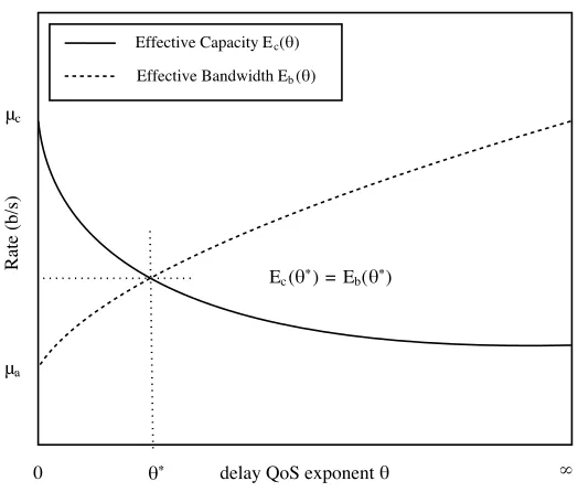
Figure 2.1: EC and EB, as functions of the delay QoS exponent θ.
lim
θ→0Eb(θ), andµc = limθ→0Ec(θ). From Fig. 2.1, it shows that when the minimum value
of EB is larger than the maximum value of EC, i.e., µa > µc, there is no solution
for θ∗ > 0 existing. In this case, the service process cannot support the required
delay QoS for the given arrival process, which is consistent with the conclusion from queueing theory that, if E[a(t)]>E[c(t)], both queue length and the queueing delay
will approach to infinity. This is because that, when θ → 0, the EB is equal to the average arrival rate of the traffic process, i.e., µa = lim
θ→0Eb(θ) =
E[a(t)]. Meanwhile,
when θ → 0, the EC is equal to the average service rate of the service process, i.e., µc = lim
θ→0Ec(θ) =
E[c(t)] [11].
In the above analysis, the buffer overflow probability was considered as the delay QoS measurements. When the focus is on the delay experienced by a source packet arriving at timet, defined byD(t), an expression analogous to (2.26) can be estimated as [10, 53]
Pr (D(t)> Dmax)≈Pr (q(t)>0)e−θµDmax, (2.27)
where Dmax denote the delay bound, and Pr (q(t)>0) is the probability of a
non-empty buffer, which can be approximated by the ratio of the average arrival rate
and the average service rate [11], i.e., E[a(t)]
E[c(t)]. Furthermore, from [11], we note that
Considering the delay violation probability in (2.27) as a function of θ, one can notice that the parameter θ plays an important role for statistical QoS guarantees, by indicating the exponential decay rate of the delay QoS violation probability [11]. A smaller θ corresponds to a slower decay rate, which implies that the system can tolerate a looser QoS guarantee, while a larger θ indicates a faster decay rate, which means that a more stringent QoS requirement can be supported. In particular, when θ →0, the system can tolerate an arbitrarily long delay. When θ → ∞, it indicates that the system cannot tolerate any delay [12].
2.2
Convex Optimization Theory
2.2.1
Convex Optimization Problems
Normally, an optimization problem has the following form [59, 60]
min f0(x) (2.28a)
subject to: fi(x)≤bi, i= 1, . . . , m (2.28b)
hi(x) = 0, i= 1, . . . , p. (2.28c)
Here, the vector x = [x1, . . . , xn] is the optimization variable of the problem, the
function f0 : Rn → R is the objective function, the functions fi : Rn → R, i =
1, . . . , m, are the inequality constraint funtions, the constantsb1, . . . , bmare the limits
for the constraints, and the functionshi :Rn→R,i= 1, . . . , pare called the equality
constraint functions [59]. If a vectorx∗ provides the minimum objective value among all feasible vectors which satisfy the constraints, then it is an optimal solution.
Then, a convex optimization problem has the following form [59]
min f0(x) (2.29a)
subject to: fi(x)≤0, i= 1, . . . , m (2.29b)
aTi x=bi, i= 1, . . . , p, (2.29c)
wheref0, . . . , fm are convex functions. Comparing (2.29) with the general form (2.28),
one can notice that the convex problem has the following requirements: 1) the objec-tive function must be convex; 2) the inequality constraint functions must be convex; 3) the equality constraint functions hi(x) = aTi x−bi must be affine [59]. Here, we
note that a function fi :Rn→R is convex if its domaindom fi is a convex set and
A functionfi is strictly convex if strict inequality holds in (2.30) whenever x6=yand
0 < α < 1. Further, a function fi is concave if −fi is convex, and strictly concave
if −fi is strictly convex. Since an affine function always holds the equality in (2.30),
therefore one can note that an affine function is both convex and concave [60]. Normally, if we can formulate a practical problem as a convex optimization prob-lem, then we can solve it efficiently. However, sometimes the formulations can be nonconvex [60]. For example, if f0 is quasiconvex instead of convex, then the
prob-lem (2.29) becomes a quasiconvex optimization probprob-lem [61]. Here, we note that a function f : Rn → R is called quasiconvex if its domain and all its sublevel sets Sα ={x ∈dom f | f(x)≤ α}, for α ∈R, are convex. The sublevel sets of convex
functions are convex, therefore convex functions are quasiconvex. But the converse is not true. For some quasiconvex problems following specific structures, e.g., convex fractional programming [62,63], they can be transformed into equivalent convex prob-lems and then get solved efficiently. The calculated optimal solutions can be proved to be optimal for the original quasiconvex problems [62, 63].
2.2.2
Lagrangian Dual and KKT Conditions
In this section, we briefly introduce the Lagrangian dual and the Karush-Kuhn-Tucker (KKT) condtions, which will be applied in Chapter 3 and Chapter 4 to solve the optimization problems and to derive the optimal power allocation strategies.
The basic idea in Lagrangian duality is to take the constraints in (2.28) into account by augmenting the objective function with a weighted sum of the constraint functions [59]. The LagrangianL:Rn×Rm×Rp →Rassociated with the problem (2.28) is defined as follows [59]
L(x, λ, v) =f0(x) +
m
X
i=1
λifi(x) + p
X
i=1
vihi(x). (2.31)
Here, λi is the Lagrangian multiplier associated with the ith inequality constraint
fi(x) ≤ 0, and vi is the Lagrangian multiplier associated with the ith equality
con-straint hi(x) = 0. The vectors λ and v are called the Lagrangian multiplier vectors
associated with the optimization problem [59].
Then, the Lagrangian dual functiong :Rm×Rp →Ris defined as the minimum
value of the Lagrangian over x: forλ∈Rm, v ∈Rp,
g(λ, v) = inf
x L(x, λ, v) = infx f0(x) +
m
X
i=1
λifi(x) + p
X
i=1
The Lagrangian dual functiong(λ, v) is concave even when the orginal problem (2.28) is not convex, since the dual function is the pointwise infimum of a family of affine functions of (λ, v) [59]. For each pair (λ, v) withλ014, the Lagrangian dual function
provides a lower bound on the optimal value p∗ of the optimization problem (2.28).
Then, in order to find the best lower bound that can be obtained from the Lagrangian function, the following optimization problem needs to be solved [59]:
max g(λ, v) (2.33a)
subject to: λ0. (2.33b)
This problem is called the Lagrangian dual problem associated with the problem (2.28). Correspondingly, the orginal problem (2.28) can be called as the primal lem. Apparently, the Lagrangian dual problem (2.33) is a convex optimization prob-lem, since the objective function is concave and the constraint function is convex [59]. This does not depend on the convexity of the primal problem (2.28) [59].
Then, we assume that the functionsf0, . . . , fm,h1, . . . , hp are differentiable. From
[59], we note that if a convex optimization problem with differentiable objective and constraint functions satisfies Slater’s condition, then the KKT conditions provide necesseary and sufficient conditions for optimality. Hence, by assuming thatfi
func-tions are convex andhi functions are affine, and x∗,λ∗, v∗ are any points that satisfy
the KKT conditions
fi(x∗)≤0, i= 1, . . . , m (2.34a)
hi(x∗) = 0, i= 1, . . . , p (2.34b)
λ∗i ≥0, i= 1, . . . , m (2.34c) λ∗ifi(x∗) = 0, i= 1, . . . , m (2.34d)
∇f0(x∗) +
m
X
i=1
λ∗i∇fi(x∗) + p
X
i=1
vi∗∇hi(x∗) = 0, (2.34e)
then x∗, λ∗,v∗ are primal and dual optimal, with zero duality gap [59].
2.3
Literature Review
2.3.1
Resource Allocation Towards Green Communications
According to International Telecommunication Union, the number of mobile subscrip-tions worldwide has dramatically increased in recent years [64]. In addition, many
14
new wireless applications, such as autonomous driving, smart cities, smart homes and appliances have emerged from research ideas to concrete systems [1]. The explosive growth of wireless communication applications coupled with the proliferation of mo-bile devices dramatically speeds up the progress of wireless networks, which results in a higher-quality human life and rapid economic growth. Meanwhile, many tech-nical challenges still remain unsolved in wireless network designs, e.g., the need for reducing energy consumption and end-to-end latency [1].
According to [65], for every 1 TeraWatt hour (TWh) energy consumption, the information and communication technology (ICT) sector is responsible for approxi-mately 0.75 million tons of CO2 gas emissions. If no action is taken, the overall costs
and risks of climate change, as a result of the increasing green house gases (GHG) emissions, will be equivalent to losing at least 5% of global gross domestic product (GDP) every year [66]. Nevertheless, it is also well known that ICT industry has the potential to reduce more than 23% of its current GHG emissions [66]. Interestingly, if one-third of the GHG emissions is reduced, the generated economical benefit will be higher than the required investment [67]. As an important part of ICT, wireless communication sector needs to take the responsibility to save more energy. Green communication technology, which emphasizes energy efficiency (EE) in addition to spectral efficiency (SE), has thereby been proposed as an effective solution which not only benefits communication technology sector, but also promotes economic and ecological sustainability. However, considering the compromise between network per-formance and energy savings, designing an efficient resource allocation strategy to limit the network energy consumption is a real challenge [68–70].
minimum system data rate requirement. EE and SE tradeoff, based on Shannon limit, has also been extensively studied for different kinds of wireless communica-tion networks, such as energy-constrained wireless multi-hop networks with a single source-destination pair [75], multi-user downlink OFDMA networks [76], general nar-rowband interference-limited systems [77] and OFDMA-based cooperative cognitive radio networks [78]. Further, the relationship between EE and SE for downlink mul-tiuser distributed antenna systems with proportional fairness was investigated in [79]. Specifically, the EE-maximization problem was first converted into a multi-objective optimization problem (MOP), by maximizing the numerator of EE while minimiz-ing its denominator. Then, the MOP was transformed into a sminimiz-ingle-objective opti-mization problem (SOP) using weighted sum method, and the optimal power value was provided by applying Lagrangian method and sub-gradient iteration approach. Considering imperfect channel estimation in an orthogonal frequency division multi-plexing (OFDM) network, the inverse of EE and inverse of SE were combined into a weighted optimization problem in [80]. The problem was then transformed into a con-vex problem, namely, to jointly minimize the total power consumption and maximize the channel capacity, which was solved using Lagrangian method.
In the aforementioned studies [75–80], Shannon limit was utilized as the system throughput, which is mostly considered as the suitable capacity metric for commu-nication systems with no link-layer delay QoS requirements. Nevertheless, for delay-sensitive mobile multimedia applications, such as video conferencing, autonomous driving and online gaming, provisioning QoS requirements is critical. Actually, 5G, the next generation of mobile communication technology, has been anticipated to not only offer>1 Gbps downlink data rate, but also sub-1ms end-to-end latency and 90% reduction in network energy usage [1]. This infers that the future wireless communica-tion networks are targeted at satisfying the end-user applicacommunica-tions’ QoS requirements, while at the same time increasing EE and SE for green communications.
a deterministic way, where the delay is bounded within a certain threshold [83]. Al-though this sounds reasonable for real-time services, satisfying fixed QoS guarantees is especially challenging in fading communication scenarios, due to the random varia-tions experienced in channel condivaria-tions, user mobility and changing environment [84], which could lead to settling for non-necessarily low data rates. In this direction, the delay-limited capacity, i.e., the zero-outage capacity, which is defined as the maximum rate achievable with a prescribed strict delay bound, was derived and analyzed in [88] and [89]. Since delay-limited capacity is a performance level that can be attained regardless of the values of the fading states, it can be seen as a stringent and deter-ministic service guarantee [84]. However, the attempt to provide a strict lower bound on delay may result in extremely conservative guarantees [10]. For example, the only lower bound that can be deterministically guaranteed in a Rayleigh fading channel is a capacity of zero [10]. In contrast to the above deterministic delay QoS bounds, in this thesis, the statistical delay QoS requirement is considered, which confines the delay bound violation probability to a required value range. In this direction, the authors in [10] introduced a link-layer capacity notion supporting statistical delay QoS requirements, which is the concept of EC.
and plotted, by expressing signal-to-noise ratio (SNR) in terms of SE using a curve fitting method in [25]. However, according to the users’ diverse preferences, vari-ous application types and dynamic surrounding circumstances, a more flexible and tractable tradeoff function is preferable, which is not provided in [22–25].