Original citation:
Gutierrez-Barragan, Felipe, Ithapu, Vamsi K., Hinrichs, Chris, Maumet, Camille, Johnson, Sterling C., Nichols, Thomas E. and Singh, Vikas. (2017) Accelerating permutation testing in voxel-wise analysis through subspace tracking : a new plugin for SnPM. NeuroImage, 159 . pp. 79-98.
Permanent WRAP URL:
http://wrap.warwick.ac.uk/90817
Copyright and reuse:
The Warwick Research Archive Portal (WRAP) makes this work by researchers of the University of Warwick available open access under the following conditions. Copyright © and all moral rights to the version of the paper presented here belong to the individual author(s) and/or other copyright owners. To the extent reasonable and practicable the material made available in WRAP has been checked for eligibility before being made available.
Copies of full items can be used for personal research or study, educational, or not-for-profit purposes without prior permission or charge. Provided that the authors, title and full bibliographic details are credited, a hyperlink and/or URL is given for the original metadata page and the content is not changed in any way.
Publisher’s statement:
© 2017, Elsevier. Licensed under the Creative Commons
Attribution-NonCommercial-NoDerivatives 4.0 International http://creativecommons.org/licenses/by-nc-nd/4.0/
A note on versions:
The version presented here may differ from the published version or, version of record, if you wish to cite this item you are advised to consult the publisher’s version. Please see the ‘permanent WRAP url’ above for details on accessing the published version and note that access may require a subscription.
Accelerating Permutation Testing in Voxel-wise Analysis
through Subspace Tracking: A new plugin for SnPM
Felipe Gutierrez-Barragana, Vamsi K. Ithapua, Chris Hinrichsa, Camille Maumetd,
Sterling C. Johnsonc, Thomas E. Nicholsd, Vikas Singhb,a,
for the Alzheimer’s Disease Neuroimaging Initiative 1
aDepartment of Computer Sciences, University of Wisconsin-Madison
bDepartment of Biostatistics & Med. Informatics, University of Wisconsin-Madison
cDepartment of Medicine, University of Wisconsin-Madison and William S. Middleton Veteran’s Hospital
dDepartment of Statistics, The University of Warwick
http://felipegb94.github.io/RapidPT/
Abstract
Permutation testing is a non-parametric method for obtaining the max null distribution used
to compute corrected p-values that provide strong control of false positives. In
neuroimag-ing, however, the computational burden of running such an algorithm can be significant. We find that by viewing the permutation testing procedure as the construction of a very
large permutation testing matrix, T, one can exploit structural properties derived from the
data and the test statistics to reduce the runtime under certain conditions. In particular,
we see that T is low-rank plus a low-variance residual. This makes T a good candidate for
low-rank matrix completion, where only a very small number of entries of T (∼ 0.35% of
all entries in our experiments) have to be computed to obtain a good estimate. Based on this observation, we present RapidPT, an algorithm that efficiently recovers the max null distribution commonly obtained through regular permutation testing in voxel-wise analysis. We present an extensive validation on a synthetic dataset and four varying sized datasets against two baselines: Statistical NonParametric Mapping (SnPM13) and a standard per-mutation testing implementation (referred as NaivePT). We find that RapidPT achieves its
best runtime performance on medium sized datasets (50≤n ≤200), with speedups of 1.5x
- 38x (vs. SnPM13) and 20x-1000x (vs. NaivePT). For larger datasets (n ≥200) RapidPT
outperforms NaivePT (6x - 200x) on all datasets, and provides large speedups over SnPM13 when more than 10000 permutations (2x - 15x) are needed. The implementation is a stan-dalone toolbox and also integrated within SnPM13, able to leverage multi-core architectures when available.
Keywords: Voxel-wise analysis, Hypothesis test, Permutation test, Matrix completion
Corresponding Author(s): Felipe Gutierrez Barragan ([email protected])
1Data used in preparation of this article was obtained from the Alzheimer’s Disease Neuroimaging
1. Introduction
Nonparametric voxel-wise analysis, e.g., via permutation tests, are widely used in the brain image analysis literature. Permutation tests are often utilized to control the family-wise error rate (FWER) in voxel-wise hypothesis testing. As opposed to parametric hypothesis testing schemes Friston et al. (1994); Worsley et al. (1992, 1996), nonparametric permutation tests Holmes et al. (1996); Nichols and Holmes (2002) can provide exact control of false positives while making minimal assumptions on the data. Further, despite the additional computational cost, permutation tests have been widely adopted in image analysis Arndt et al. (1996); Halber et al. (1997); Holmes et al. (1996); Nichols and Holmes (2002); Nichols and Hayasaka (2003) via implementations in broadly used software libraries available in the community SnPM (2013); FSL (2012); Winkler et al. (2014).
Running time aspects of Permutation Testing. Despite the varied advantages of
permuta-tion tests, there is a general consensus that the computapermuta-tional cost of performing permutapermuta-tion tests in neuroimaging analysis can often be quite high. As we will describe in more detail
shortly, high dimensional imaging datasets essentially mean thatfor each permutation,
hun-dreds of thousands of test statistics need to be computed. Further, as imaging technologies continue to get better (leading to higher resolution imaging data) and the concurrent slow-down in the predicted increase of processor speeds (Moore’s law), it is reasonable to assume that the associated runtime will continue to be a problem in the short to medium term. To alleviate these runtime costs, ideas that rely on code optimization and parallel computing have been explored Eklund et al. (2011); A. Eklund (2012, 2013). These are interesting strategies but any hardware-based approach will be limited by the amount of resources at
hand. Clearly, significant gains may be possible if more efficient schemes that exploit the
underlying structure of the imaging data were available. It seems likely that such algorithms can better exploit the resources (e.g., cloud or compute cluster) one has available as part of a study and may also gain from hardware/code improvements that are being reported in the literature.
(2008), albeit the objective there is to obtain a less conservative correction, rather than com-putational efficiency. Recently, motivated by neuroimaging applications and comcom-putational issues, Gaonkar and Davatzikos (2013) derived an analytical approximation of statistical sig-nificance maps to reduce the computational burden imposed by permutation tests commonly used to identify which brain regions contribute to a Support Vector Machines (SVM) model. In summary, exploiting the structure of the data to obtain alternative efficient solutions is
not new, but we find that in the context of permutation testing on imaging data, there is
a great deal of voxel-to-voxel correlations that if leveraged properly can, in principle, yield interesting new algorithms.
For permutation testing tasks in neuroimaging in particular, several groups have recently investigated ideas to make use of the underlying structure of the data to accelerate the procedure. In a preliminary conference paper (Hinrichs et al. (2013)), we introduced the notion of exploiting correlations in neuroimaging data via the underlying low-rank structure of the permutation testing procedure. A few years later, Winkler et al. (2016) presented the first thorough evaluation of the accuracy and runtime gains of six approaches that leverage the problem structure to accelerate permutation testing for neuroimage analysis. Among these approaches Winkler et al. (2016) presented an algorithm which relied on some of the ideas introduced by Hinrichs et al. (2013) to accelerate permutation testing through low-rank matrix completion (LRMC). Overall, algorithms that exploit the underlying structure of permutation testing in neuroimaging have provided substantial computational speedups.
1.1. Main Idea and Contributions
The starting point of our formulation is to analyze the entire permutation testing pro-cedure via numerical linear algebra. In particular, the object of interest is the permutation
testing matrix, T. Each row of T corresponds to the voxel-wise statistics, and each
col-umn is a specific permutation of the labels of the data. This perspective is not commonly used because a typical permutation test in neuroimaging rarely instantiates or operates on
this matrix of statistics. Apart from the fact that T, in neuroimaging, contains millions
of entries, the reason for not working directly with it is because the goal is to derive the
maximum null distribution. The central aspect of this work is to exploit the structure in T
– the spatial correlation across different voxel-statistics. Such correlations are not atypical because the statistics are computed from anatomically correlated regions in the brain. Even far apart voxel neighbourhoods are inherently correlated because of the underlying biological structures. This idea drives the proposed novel permutation testing procedure. We describe the contributions of this paper based on the observation that the permutation testing matrix is filled with related entries.
• Theoretical Guarantees. The basic premise of this paper is thatpermutation testing
in high-dimensions (especially, imaging data) is extremely redundant. We show how we
can modelTas a low-rank plus a low-variance residual. We provide two theorems that
support this claim and demonstrate its practical implications. Our first result justifies
this modeling assumption and several of the components involved in recoveringT. The
second result shows that the error in the global maximum null distribution obtained
• A novel, fast and robust, multiple-hypothesis testing procedure. Building upon the theoretical development, we propose a fast and accurate algorithm for permu-tation testing involving high-dimensional imaging data. The algorithm achieves state
of the art runtime performance by estimating (or recovering) the statistics inTrather
than “explicitly” computing them. We refer to the algorithm as RapidPT, and we
show that compared to existing state-of-the-art libraries for non-parametric testing,
the proposed model achieves approximately 20× speed up over existing procedures.
We further identify regimes where the speed up is even higher. RapidPT also is able to leverage serial and parallel computing environments seamlessly.
• A plugin in SnPM (with stand-alone libraries). Given the importance and
the wide usage of permutation testing in neuroimaging (and other studies involving high-dimensional and multimodal data), we introduce a heavily tested implementa-tion of RapidPT integrated as a plugin within the current development version of SnPM — a widely used non-parametric testing toolbox. Users can invoke RapidPT directly from within the SnPM graphical user interface and benefit from SnPM’s fa-miliar pre-processing and post-processing capabilities. This final contribution, with-out a separate installation, brings the performance promised by the theorems to the neuroimaging community. Our documentation Gutierrez-Barragan and Ithapu (2016) gives an overview of how to use RapidPT within SnPM.
Although the present work shares some of the goals and motivation of Winkler et al.
(2016) – specifically, utilizing the algebraic structure of T – there are substantial technical
differences in the present approach, which we outline further below. First, unlike Winkler et al. (2016), we directly study permutation testing for images at a more fundamental level and seek to characterize mathematical properties of relabeling (i.e., permutation) procedures operating on high-dimensional imaging data. This is different from assessing whether the underlying operations of classical statistical testing procedures can be reformulated (based on the correlations) to reduce computational burden as in Winkler et al. (2016). Second, by exploiting celebrated technical results in random matrix theory, we provide theoretical
guarantees for estimation and recovery of T. Few such results were known. Note that
em-pirically, our machinery avoids a large majority of the operations performed in Winkler et al. (2016). Third, some speed-up strategies proposed in Winkler et al. (2016) can be considered as special cases of our proposed algorithm — interestingly, if we were to increase the number
‘actual’ operations performed by RapidPT (from ≈ 1%, suggested by our experiments, to
50%), the computational workload begins approaching what is described in Winkler et al. (2016).
2. Permutation Testing in Neuroimaging
In this section, we first introduce some notations and basic concepts. Then, we give additional background on permutation testing for hypothesis testing in neuroimaging to motivate our formulation. Matrices and vectors will be denoted by bold upper-case and lower-case letters respectively, and scalars will be represented using non-bold letters. For
a matrix X, X[i,:] denotes the ith row and X[i, j] denotes the element in ith row and jth
Permutation testing is a nonparametric procedure for estimating the empirical distribu-tion of the global null Edgington (1969b,a); Edgington and Onghena (2007). For a
two-sample univariate statistical test, a permutation test computes an unbiased estimate of the
null distribution of the relevant univariate statistic (e.g., t or χ2). Although univariate
null distributions are, in general, well characterized, the sample maximum of the voxel-wise statistics usually does not have an analytical form due to strong correlations across voxels, as discussed in Section 1. Permutation testing is appropriate in this high-dimensional setting because it is non-parametric and does not impose any restriction on the correlations across the voxel-wise statistics. Indeed, when the test corresponds to group differences between
samples based on a stratification variable, under the null hypothesis H0, the grouping labels
given to the samples are artificial, i.e., they correspond to the set of all possiblerelabellingsof
the samples. In neuroimaging studies, typically the groups correspond to the presense or
ab-sence of an underlying disease condition (e.g., controls and diseased). WheneverH0 is true,
the data sample representing a healthy subject is, roughly speaking, ‘similar’ to a diseased
subject. Under this setting, in principle, interchanging the labels of the two instances will
have no effect on the distribution of the resulting voxel-wise statistics across all the dimen-sions (or covariates or features). So, if we randomly permute the labels of the data instances
from both groups, under H0 the recomputed sets of voxel-wise statistics correspond to the
same global null distribution. We denote the number of such relabellings (or permutations)
by L. The histogram of all L maximum statistics i.e., the maximum across all voxel-wise
statistics for a given permutation, is the empirical estimate of the exact maximum null
dis-tribution under H0. When given the true/real labeling, to test for significant group-wise
differences, one can simply compute the fraction of the max null that is more extreme than the maximum statistic computed across all voxels for this real labeling.
The case for strong null. Observe that when testing multiple sets of hypotheses there
are two different types of control for the Type 1 error rate (FWER): weak and strong con-trol Y. Hochberg (1987). A test is referred to as weak concon-trol for FWER whenever the Type 1 error rate is controlled only when all the hypotheses involved (here, the number of
voxels being tested) are true. That is, H0 is true for (all) voxels. On the other hand, a
test provides strong control for FWER whenever Type 1 error rate is controlled under any combination/proportion of the true hypotheses. It is known that the procedure described above (i.e., using the max null distribution calculated across all voxel-wise statistics) provides strong control of FWER Holmes et al. (1996). This is easy to verify because the maximum
of all voxel-wise statistics is used to compute the correctedp-value, and so, the exact
propor-tion of which hypotheses are true does not matter. Further, testing based on strong control
will classify non-activated voxels as activated with a probability upper bounded by α, i.e.,
it has localizing power Holmes et al. (1996), a desirable property in neuroimaging studies in particular. For the remainder of this paper, we will focus on such strong control and restrict our presentation to the case of group difference analysis for two groups.
2.1. NaivePT: The exhaustive Permutation Testing procedure
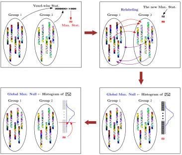
Figure 1 and algorithm 1 illustrate the permutation testing procedure. Given the data
instances from two groups, X1 ∈
Rv×n1 and X2 ∈
Rv×n2, where n
1 and n2 denote the
in the brain image. Let n = n1 +n2 and X = [X1;X2] give the (row-wise) stacked data
matrix (X ∈ Rv×n). Note that a permutation of the columns of X corresponds to a group
relabelling. The v distinct voxel-wise statistics are then computed for Lsuch permutations,
and used to construct the permutation testing matrix T ∈ Rv×L. The empirical estimate
of the max null is simply the histogram of the maximum of each of the columns of T –
denoted by hL. Algorithm 1 is occasionally referred to as Monte Carlo permutation tests
in the literature because of the random sampling involved in generating the statistics. This standard description of a permutation test will be used in the following sections to describe our proposed testing algorithm.
Group1 Group2
Max. Stat.
Voxel-wise Stat.
Group1 Group2
Relabeling The new Max. Stat.
Group1 Group2 Global Max. Null←Histogram of Group1 Group2
[image:7.612.123.489.219.531.2]Global Max. Null←Histogram of
Figure 1: Flow diagram of the permutation testing procedure described in algorithm 1. Group 1 and Group 2 correspond toX1andX2, each new max stat corresponds to eachm
i, and the global max null corresponds
tohL.
2.2. The situation when L is large
Evidently as the number of permutations (L) increases Algorithm 1 becomes extremely
expensive. Nonetheless, performing a large number of permutations is essential in neuroimag-ing for various reasons. We discuss these reasons in some detail next.
1) Random sampling methods draw many samples from near the mode(s) of the distribution
Algorithm 1 NaivePT The exhaustive permutation testing procedure.
Input: X1,X2,L
Output: T, hL
X= [X1;X2],n =n 1+n2
m1. . . , mL←[∅]
for i∈1, . . . , L do
j1. . . , jn ∼Permute[1, n]
˜
X1 ←X[:, j
1, . . . , jn1], ˜X
2 ←X[:, j
n1+1, . . . , jn]
T[:, i]←test( ˜X1,X˜2)
mi ←Max(T[:, i])
end for
hL ←Histogram(m1, . . . , mL)
samples just so that the estimate converges. So, if we want an α = 0.01 threshold
from the max null distribution, we require many thousands of permutation samples — a computationally expensive procedure in neuroimaging as previously discussed.
2) Ideally we want to obtain a precise threshold for any α, in particular small α. However,
the smallest possiblep-value that can be obtained from the empirical null is L1. Therefore,
to calculate very low p-values (essential in many applications), L must be very large.
3) A typical characteristic of brain imaging disorders, for instance in theearly(e.g.,
preclin-ical) stages of Alzheimer’s disease (AD) and other forms of dementia, is that the disease signature is subtle — for instance, in AD, the deposition of Amyloid load estimated via positron emission tomographic (PET) images or atrophy captured in longitudinal struc-tural magnetic resonance images (MRI) image scans in the asymptomatic stage of the disease. The signal is weak in this setting and requires large sample size studies (i.e.,
largen) and a need for estimating the Type 1 error threshold with high confidence. The
necessity for high confidence tail estimation implies that we need to sample many more
relabelings, requiring a large number of permutationsL.
3. A Convex Formulation to characterize the structure of T
It turns out that the computational burden of algorithm 1 can be mitigated by exploiting
the structural properties of the permutation testing matrixT. Our strategy uses ideas from
LRMC, subspace tracking, and random matrix theory, to exploit the correlated structure of
T and model it in an alternative form. In this section, we first introduce LRMC, followed
by the overview of the eigen-spectrum propoerites of T, which then leads to our proposed
model of T.
3.1. Low-Rank Matrix Completion
Given only a small fraction of the entries in a matrix, the problem of low-rank matrix
completion (LRMC) Cand`es and Tao (2010) seeks to recover the missing entries of the
entire matrix. Clearly, with no assumption on the properties of the matrix, such a recovery
is ill-posed. Instead, if we assume that the column space of the matrix is low-rank and
and others have shown that, with sufficiently small number of entries, one can recover the orthogonal basis of the row space as well as the expansion coefficients for each column — that is, fully recover the missing entries of the matrix. Specifically, the number of entries required
is roughly rlog(d) where r is the column space’s rank and d is the ambient dimension. By
placing an`1-norm penalty on the eigenvalues of the recovered matrix, i.e., the nuclear norm
Fazel et al. (2004); Recht et al. (2010), one optimizes a convex relaxation of an (non-convex) objective function which explicitly minimizes the rank. Alternatively, we can specify a rank
r ahead of time, and estimate an orthogonal basis of that rank by following a gradient along
the Grassmannian manifold Balzano et al. (2010); He et al. (2012). The LRMC problem has received a great deal of attention in the period after the Netflix Prize Bennett and Lanning (2007), and numerous applications in machine learning and computer vision have been investigated Ji et al. (2010). Details regarding existing algorithms and their analyses
including strong recovery guarantees are available in Cand`es and Recht (2009); Recht (2011).
LRMC Formulation. Let us consider a matrixT∈Rv×L. Denote the set of randomly
subsampled entries of this matrix as Ω. This means that we have access to TΩ, and our
recovery task corresponds to estimating TΩC, where ΩC corresponds to the complement of
the set Ω. Let us denote the estimate of the complete matrix be ˆT. The completion problem
can be written as the following optimization task,
min
ˆ T
kTΩ−TˆΩk2Frob (1)
s.t. Tˆ =UW (2)
U is orthogonal. (3)
where U ∈ Rv×r is the low-rank basis of T, i.e., the columns of U correspond to the
orthogonal basis vectors of the column space of T. Here, Ω gives the measured entries
and W is the matrix of coefficients that lets us reconstruct ˆT.
3.2. Low-rank plus a long tail in T
Most datasets encountered in the real world (and especially in neuroimaging) have a
dominant low-rank component. While the data may not be exactly characterized by a
low-rank basis, the residual will not significantly alter the eigen-spectrum of the sample covariance in general. Strong correlations nearly always imply a skewed eigen-spectrum, because as the the eigen-spectrum becomes flat, the resulting covariance matrix tends to become sparser (the “uncertainty principle” between low-rank and sparse matrices Chandrasekaran et al. (2011)). Low-rank structure in the data is encountered even more frequently in neuroimaging — unlike natural images in computer vision, there is much stronger voxel-to-voxel homogeneity in a brain image.
While performing statistical hypothesis testing on these images, the low-rank structure
described above carries through toTfor purely linear statistics such as sample means, mean
differences and so on. However, non-linearities in the test statistic, e.g., normalizing by pooled variances, will perturb the eigen-spectrum of the original data, contributing a long tail of eigenvalues (see Figure 2). This large number of significant singular values needs to
be accounted for, if one intends to model T using low-rank structure. Ideally, we require
eigenvalues. This is equivalent to asking that the resulting non-linearities do notdecorrelate
the test statistics, to the point that the matrix T cannot be approximated by a low-rank
matrix with high fidelity. For t-statistics, the non-linearities come from normalization by
pooled variances, see for example a two-sample t-test shown in (4). Here (µ1, σ1) and (µ2,
σ2) are the mean and standard deviations for the two groups respectively. Since the pooled
variances calculated from correlated data X are unlikely to change very much from one
permutation sample to another (except outliers), we expect that the spectrum of T will
resemble that of the data (or sample) covariance, with the addition of a long, exponentially
decaying tail. More generally, if the non-linearity does not decorrelate the test statistics too
much, it will almost certainly preserve the low-rank structure.
t= qµ1−µ2
σ1
n1 +
σ2
n2
(4)
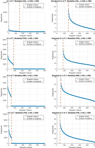
Does low-rank plus a long tail assumption hold for other image modalities? The underlying thesis of our proposed framework is that the permutation testing matrix
T, in general, has this low-rank plus long tail structure. In Figure 2, we show evidence that
this is in fact the case for a variety of imaging modalities that are commonly used in med-ical studies – Arterial Spin Labeling (ASL), Magnetic Resonance Imaging (MRI), and two Positron Emission Tomography (PET) modalities including fluorodeoxyglucose (FDG) and Pittsburgh compound B (PiB). Using several images coming from each of these modalities
four differentTs are constructed. Each row in Figure 2 shows the decay of the singular value
spectrum of these four differentTs. The low-rank (left column) and the remaining long tail
(right column) is clearly seen in these spectrum plots which suggests that the core modeling assumptions are satisfied. We note that the MRI data that was used in Figure 2 was in fact the de facto dataset for our evaluation presented in section 6. The underlying construct of such high correlations across multiple covariates or predictors is common to most biological datasets beyond brain scans, like genetic datasets.
3.3. Overview of Proposed method
If the low-rank structure dominates the long tail described above, then its contribution
to Tcan be modeled as a low variance Gaussian i.i.d. residual. A Central Limit argument
appeals to the number of independent eigenfunctions that contribute to this residual, and, the orthogonality of eigenfunctions implies that as more of them meaningfully contribute to each entry in the residual, the more independent those entries become. In other words, if this long tail begins at a low magnitude and decays slowly, then we can treat it as a
Gaussian i.i.d. residual; and if it decays rapidly, then the residual will perhaps be less
Gaussian, but also more negligible. Thus, our algorithm makes no direct assumption about
these eigenvalues themselves, but rather that the residual corresponds to a low-variancei.i.d.
Gaussian random matrix – its contribution to the covariance of test statistics will beWishart
distributed, and from this property, we can characterize its eigenvalues.
Why should we expect runtime improvements? The low-rank + long tail structure
of the permutation testing matrix then translates to the following identity,
0 100 200 300 400 500
Singular Values
0 5000 10000 15000
Magnitude
S.V of T: Modality=ASL, n=150, L=500
Singular Values Number of Subjects
0 100 200 300 400 500
Singular Values
0.5 1 1.5 2 2.5 3 3.5 4
Magnitude
Residual S.V of T: Modality=ASL, n=150, L=500
Singular Values Number of Subjects
0 100 200 300 400 500
Singular Values
0 1000 2000 3000 4000 5000 6000
Magnitude
S.V of T: Modality=FDG, n=80, L=500
Singular Values Number of Subjects
0 100 200 300 400 500
Singular Values
5 10 15 20 25 30
Magnitude
Residual S.V of T: Modality=FDG, n=80, L=500
Singular Values Number of Subjects
0 100 200 300 400 500
Singular Values
0 1000 2000 3000 4000 5000
Magnitude
S.V of T: Modality=MRI, n=50, L=500
Singular Values Number of Subjects
0 100 200 300 400 500
Singular Values
10 15 20 25 30
Magnitude
Residual S.V of T: Modality=MRI, n=50, L=500
Singular Values Number of Subjects
0 100 200 300 400 500
Singular Values
0 2000 4000 6000 8000 10000
Magnitude
S.V of T: Modality=PiB, n=40, L=500
Singular Values Number of Subjects
0 100 200 300 400 500
Singular Values
10 20 30 40 50 60 70
Magnitude
Residual S.V of T: Modality=PiB, n=40, L=500
[image:11.612.116.477.73.635.2]Singular Values Number of Subjects
Figure 2: Singular value spectrums for permutation testing matrices with dimensions generated from the imaging modalities: ASL, FDG PET, MRI, and PiB PET. Left: Full spectrum of T with L rows and v
where S is the unknown i.i.d. Gaussian random matrix. We do not restrict ourselves to
one-sided tests here, and so, S is modeled to be zero-mean. Later in Section 4, we show
that this apparent zero-mean assumption is addressed because of a post-processing step.
The low-rank portion of Tcan be reconstructed by sub-sampling the matrix at Ω using the
LRMC optimization from (1). Recall from the discussion in Section 3.1 that Ω corresponds
to a subset of indices of the entries inT, i.e., instead of computing all voxel-wise statistics for
a given relabeling (a column of T), only a small fraction η, referred to as the sub-sampling
rate, are computed. Later in Sections 5 and 6, we will show that η is very small (on the
orders of < 1%). Therefore, the overall number of entries in Ω — the number of statistics
actually calculated to recover T – is ηvL as opposed to vL forη 1.
Since the core of the proposed method is to model T by accessing only a small subset of
its entries Ω, we refer to it as a rapid permutation testing procedure – RapidPT. Observe
that a large contributor to the running time of online subspace tracking algorithms, including
the LRMC optimization from (1), is the module which updates the basis set U; but once a
good estimate forUhas been found, this additional calculation is no longer needed. Second,
the eventual goal of the testing procedure is to recover the max null as discussed earlier in
Section 2, which then implies that the residual Sshould also be recovered with high fidelity.
Exact recovery ofSis not possible. Although, for our purposes, we only need its effect on the
distribution of the maximumper permutation test. An estimate of the mean and variance of
S then provides reasonably good estimates of the max null. We therefore divide the entire
process into two steps: training, andrecoverywhich is described in detail in the next section.
4. Rapid Permutation Testing – RapidPT
In this section, we discuss the specifics of the training and recovery stages of RapidPT,
and then present the complete algorithm, followed by some theoretical guarantees regarding
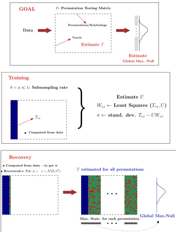
consistency and recovery of T. Figure 3 shows a graphical representation of the RapidPT
algorithm 2.
4.1. The training phase
The goal of the training phase is to estimate the basis U. Here, we perform a small
number of fully sampled permutation tests, i.e., for approximately a few hundred of the
columns of T (each of which corresponds to a permutation) denoted by `, all the v
voxel-wise statistics are computed. Thisv×` “sub-matrix” ofT is referred to as thetraining set,
denoted byTex. In our experiments,`was selected to be either a fraction or a multiple of the
total number of subjects n as described in section 5.4. From Tex, we estimate the basis U
using sub-sampled matrix completion methods Balzano et al. (2010); He et al. (2012), making
multiplepasses over the training set with the (given) sub-sampling rate η, until convergence.
This corresponds to initializingU as a random orthogonal matrix of a pre-determined rank
r, and using the columns of Tex repeatedly to iteratively update it until convergence (see
Balzano et al. (2010); He et al. (2012) for details regarding subspace tracking). Once U
is obtained in this manner, Wex is obtained by running a simple least-squares procedure
on Tex and U. The histogram of Tex −UWex will then be an estimate of the empirical
distribution of the residual S over the training set. We denote the standard deviation of
Notice that in principle, one can estimate U directly from Tex by simply computing
the leading r principal components. This involves a brute-force approximation of U by
computing the singular-value decomposition of a dense v ×` matrix. Even for reasonably
small v, this is a costly operation. Second, ˆT, by definition, contains a non-trivial residual.
We have no direct control on the structure of S except that it is i.i.d Gaussian. Clearly,
the variance of entries of S will depend on the fidelity of the approximation provided by
U. Since the sub-sampling rateη (the size of the set Ω compared to vL) is known ahead of
time, estimating U via a subspace-tracking procedure using η fraction of the entries of Tex
(where each column ofTex modifies an existing estimate ofU, one-by-one, without requiring
to store all the entries of Tex) directly provides an estimate of S.
Bias-Variance Trade-off. When using a very sparse subsampling method i.e., sampling
with small η, there is a bias-variance trade-off in estimating S. Clearly, if we use the entire
matrix T to estimate U, W and S, we will obtain reliable estimates of S. But, there is
an overfitting problem: the least-squares objective used in fitting W (in getting a good
estimate of the max null) to such a small sample of entries is likely to grossly underestimate
the variance of S compared to when we use the entire matrix; the sub-sampling problem is
not nearly as over-constrained as it is for the full matrix. This sampling artifact reduces
the apparent variance of S, and induces a bias in the distribution of the sample maximum,
because extreme values are found less frequently. This sampling artifact has the effect of “shifting” the distribution of the sample maximum towards zero. We refer to this as a bias-variance trade-off because, we can think of the need for shift as an outcome of the
sub-optimality of the estimate of σ versus the deviation of the true max null from the estimated
max null, We correct for this bias by estimating the amount of the shift during the training phase, and then shifting the recovered sample max distribution by this estimated amount.
This shift is denoted by µ.
4.2. The recovery phase
In the recovery phase, we sub-sample a small fraction of the entries of each column of
T successively, i.e., for each new relabeling, the voxel-wise statistics are computed over a
small fraction of all the voxels to populate TΩ. Using this TΩ, and the pre-estimated U,
the reconstruction coefficients for this column w ∈ Rr×1 are computed. After adding the
random residuals – i.i.d Gaussian with mean µ and standard deviation σ, to this Uw, we
have our estimate ˆT for this specific relabeling/permutation. Recall that S was originally
modeled to be zero-mean (see (5)), but the presence of the shift µ suggests a N(µ, σ2)
distribution instead. Overall, this entails recovering a total of v voxel-wise statistics from
ηv of such entries where η 1. This process repeats for all the remaining L−` columns
of T, eventually providing ˆT. Once ˆT has been estimated, we proceed exactly as in the
NaivePT, to compute the max null and test for the significance of the true labeling.
4.3. The Algorithm
Algorithm 2 and Figure 3 summarizes RapidPT. The algorithm takes in the input data
X, the rank of the basisr, the sub-sampling rateη, the number of training columns`and the
total number of columns Las inputs, and returns the estimated permutation testing matrix
Computed from data
Permutations/Relabelings
Voxels
T: Permutation Testing Matrix
GOAL
Data
Estimate
Training
EstimateT
Global Max. Null
Tex
0< η1: Subsampling rate
}
Estimate UWex← Least Squares (Tex, U)
σ← stand. dev. Tex−U Wex
Computed from data – to get w
Recovered:= Uw + ∼ N(0, σ2) T estimated for all permutations
Recovery
[image:14.612.120.482.74.552.2]Max. Stats. for each permutationGlobal Max-Null
Figure 3: Flow diagram of the training and recovery steps in RapidPT. The number of training samples (l) and the rank ofU(r) is the number of columns computed in the training phase (the blue area). The sub-sampling rate,η, is the fraction of red over green entries computed per column. The global max null is
hL in the algorithm.
2 first estimates U, σ and the shift µ, which are then used to compute W and S for the L
number of permutations.
4.4. Summary of theoretical guarantees
Algorithm 2 shows an efficient way to recover the max null by modeling T as a
Algorithm 2 The RapidPT algorithm for permutation testing.
Input: X1,X2,r,η,L, `, stat
Output: Tˆ, hL
X= [X1;X2],n =n 1+n2
TRAINING
U←Rand. Orth., Wex = [∅] for i∈1, . . . , `do
j1. . . , jn ∼Permute[1, n]
˜
X1 ←X[:, j1, . . . , jn1]
˜
X2 ←X[:, j
n1+1, . . . , jn]
Tex[:, i]←test( ˜X1,X˜2)
k1, . . . , kdηve∼UNIF[1, v]
˜
T←Tex[k1, . . . , kdηve, i]
U,Wex[:, i]←Subspace-Tracking(r)
end for
σ←Standard Deviation{Tex−UWex}Ω
µ←supiMax{Tex[:, i]−UWex[:, i]}
for i∈1, . . . , `do ˆ
T[:, i]←T[:, i] end for
RECOVERY
for i∈`+ 1, . . . , L do
k1, . . . , kdηve∼UNIF[1, v]
j1. . . , jn ∼Permute[1, n]
˜
X1 ←X[k
1, . . . , kdηve, j1, . . . , jn1]
˜
X2 ←X[k
1, . . . , kdηve, jn1+1, . . . , jn]
˜
T←test( ˜X1,X˜2)
W[:, i]←Complete(U,T˜, k1, . . . , kdηve) s←i.i.dNv(0, σ2)
ˆ
T[:, i]←UW[:, i] +s end for
for i∈1, . . . , L do
if i≤` then
mi ←Max( ˆT[:, i])
else
mi ←Max( ˆT[:, i]) +µ
end if end for
hL ←
Histogram(m1, . . . , mL)
of the results is (1) the basic model (i.e., low-rank and low-variance residual) is indeed meaningful for the setting we are interested in, and (2) Recovering the low-rank and the residual by Algorithm 2 guarantees a high fidelity estimate of the max null, and shows that the error is small.
5. Experimental Setup
We evaluate RapidPT in multiple phases. First we perform a simulation study where the goal is to empirically demonstrate the requirements on the input hyperparameters that will guarantee an accurate recovery of the max null. These empirical results are compared to the analytical bounds governed by the theory (and further discussed in the supplement). The purpose of these evaluations is to walk the reader through the choices of hyperparameters, and how the algorithm is very robust to them. Next, we perform another simulation study where our goal is to evaluate the performance of RapidPT on multiple synthetic datasets generated by changing the strength of group-wise differences and the sparsity of the signal (e.g., how many voxels are different). We then conduct an extensive experiments to evaluate RapidPT against competitive methods on real brain imaging datasets. These include com-parisons of RapidPT’s accuracy, runtime speedups and overall performance gains against two baselines. The first baseline we used was the latest release of the widely used MATLAB toolbox for nonparametric permutation testing in neuroimaging, Statistical NonParametric Mapping (SnPM) (SnPM (2013); Nichols and Holmes (2002)). The second baseline was a standard MATLAB implementation of algorithm 1, which we will call NaivePT. Both base-lines serve to evaluate RapidPT’s accuracy. Further, the very small differences between the results provided by SnPM and NaivePT offer a secondary reference point that tells us an acceptable range for RapidPT’s results (in terms of differences). For runtime performance, SnPM acts as a state of the art baseline. On the other hand, NaivePT is used to evaluate how an unoptimized permutation testing implementation will perform on the datasets we use in our experiments. In the next section, we describe the experimental data, the hyper-parameters space evaluated, the methods used to quantify accuracy, and the environment where all experiments were run.
5.1. Simulation Data I
The dataset consisted of n = 30 synthetic images composed of v = 20000 voxels. The
signal in each voxel is derived from one of the following two normal distributions: N(µ =
0, σ2 = 1) and N(µ= 1, σ2 = 1). Two groups were then constructed with 15 images in each
and letting 1% (200 voxels) exhibit voxel-wise group differences. The signal in the remaining
99% of the voxels was assumed to come from N(µ= 0, σ2 = 1).
5.2. Simulation Data II
The dataset consisted of a total of 48 synthetically generated datasets, each with v =
20000 voxels. The datasets were generated by varying: the number of images (n) in the
dataset, the strength of the signal (i.e., deviation of µ in N(µ,1) from N(0,1)) and the
sparsity of the signal (percentage of voxels showing group differences). The dataset sizes
were n = 60, n = 150, n = 600. Each dataset was split into two equally sized groups for
datasets. The first “group” (for group-difference analysis) in all datasets was generated
from a standard normal distribution, N(µ = 0, σ2 = 1). In the second “group”, we chose
{1%,5%,10%,25%} of the voxels from one of four normal distributions (N(µ= 1, σ2 = 1),
N(µ = 5, σ2 = 1), N(µ = 10, σ2 = 1), N(µ = 25, σ2 = 1)). The signal in the remaining
voxels in the second group was also obtained from N(µ= 0, σ2 = 1).
To summarize the simulation setup, Simulation Data I fixes the dataset and changes the algorithmic hyperparameters whereas Simulation Data II fixes the algorithmic hyperparam-eters and generates different datasets.
5.3. Data
The data used to evaluate RapidPT comes from the Alzheimer’s disease Neuroimaging Initiative-II (ADNI2) dataset. The ADNI project was launched in 2003 by the National In-stitute on Aging, the National InIn-stitute of Biomedical Imaging and Bioengineering, the Food and Drug Administration, private pharmaceutical companies, and nonprofit organizations, as a $60 million, 5-year public-private partnership. The overall goal of ADNI is to test whether serial MRI, positron emission tomography (PET), other biological markers, and clinical and neuropsychological assessment can be combined to measure the progression of MCI and early AD. Determination of sensitive and specific markers of very early AD progression is intended to aid researchers and clinicians to develop new treatments and monitor their effectiveness, as well as lessen the time and cost of clinical trials. The principal investigator of this ini-tiative is Michael W. Weiner, M.D., VA Medical Center and University of California — San Francisco. ADNI is the result of the efforts of many co-investigators from a broad range of academic institutions and private corporations, and subjects have been recruited from over 50 sites across the U.S. and Canada. The initial aim of ADNI was to recruit 800 adults, ages 55 to 90, to participate in the research — approximately 200 cognitively normal older individuals to be followed for 3 years, 400 people with MCI to be followed for 3 years, and 200 people with early AD to be followed for 2 years.
For the experiments presented in this paper, we used gray matter tissue probability maps derived from T1-weighted magnetic resonance imaging (MRI) data. From this data,
we constructed four varying sized datasets. We sampled n1 and n2 subjects from the CN
and AD groups in the cohort, respectively. Table 1 shows a summary of the datasets used for our evaluations.
Dataset Size: n (n1,n2)
50 (25,25) 100 (50,50) 200 (100,100) 400 (200,200)
Table 1: Dataset sizes used in our experiments. The table lists the total number of subjects (n) and how many of the participants were sampled from the CN (n1) and AD groups (n2).
5.3.1. Data Pre-processing
All images were pre-processed using voxel-based morphometry (VBM) toolbox in Sta-tistical Parametric Mapping software (SPM, http://www.fil.ion.ucl.ac.uk/spm). After
pre-processing, we obtain a data matrixX composed of n rows and v columns for each dataset
shown in Table 1. Each row inX corresponds to a subject and each column is associated to
images are already co-registered). This pre-processing is commonly used in the literature and not specialized to our experiments.
5.4. Hyperparameters
As outlined in Algorithm 2, there are three high-level input parameters that will impact
the performance of the procedure: thenumber of training samples (l), the sub-sampling rate
(η), and thenumber of permutations (L). To demonstrate the robustness of the algorithm to
these parameter settings, we explored and report on hundreds of combinations of these hy-perparameters on each dataset. This also helps us identify the general scenarios under which RapidPT will be a much superior alternative to regular permutation testing. The baselines for a given combination of these hyperparameters are given by the max null distribution constructed by SnPM and NaivePT. The number of permutations used for the max null distributions of the baselines is the same as the number of permutations used by RapidPT for a given combination of hyperparameters.
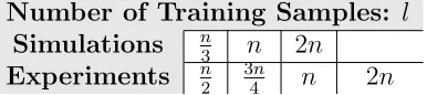
• Number of Training Samples: The number of training samples,l, determines how many
columns of Tare calculated to estimate the basis of the subspace, and also how many
training passes are performed to estimate the shift that corrects for the bias-variance
tradeoff discussed in Section 4.1. We decided to use the total number of subjects n as
a guide to pick a sensible l, the rationale is that the maximum possible rank ofT is n
(as discussed in Section 3). Further, l is also used to determine the number of passes
performed to calculate the shift of the max null distribution. Calculating the shift is
a cheap step, therefore it makes sense to use all the information available in Tex to
calculate the shift. Table 2 shows a summary of the different values for l used in our
evaluations.
Number of Training Samples: l
Simulations n3 n 2n
[image:18.612.212.405.444.487.2]Experiments n2 3n4 n 2n
Table 2: Number of training samples used to evaluate RapidPT. n corresponds to the total number of subjects in the dataset. For instance, for the 400 subject dataset the values for l used were 100, 200, 400, and 800.
• Sub-sampling rate: The sub-sampling rate, η, is the percentage of all the entries of
T that we will calculate (i.e., sample) when recovering the max null distribution. In
the recovery phase,η determines how many voxel-wise test statistics will be calculated
at each permutation to recover a column of ¯T. For instance, if the data matrix has
v columns (number of voxels) then instead of calculating v test statistics, we will
sample only ηv (where η 1) random columns and calculate test statistics only for
those columns. Table 3 shows a summary of the different values for η used in our
evaluations.
• Number of Permutations The number of permutations,L, determines the total number
of columns inT. By varyingLwe are able to see how the size ofTaffects the accuracy
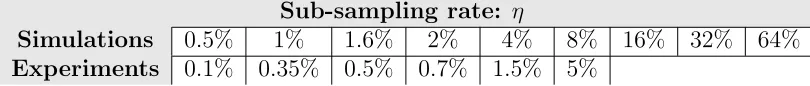
Sub-sampling rate: η
Simulations 0.5% 1% 1.6% 2% 4% 8% 16% 32% 64%
[image:19.612.105.510.73.116.2]Experiments 0.1% 0.35% 0.5% 0.7% 1.5% 5%
Table 3: Sub-sampling rates used to evaluate RapidPT.ηis the percentage of the total number of entries in
Tthat will be calculated during the recovery phase.
implementation with the same number of permutations (e.g., NaivePT or SnPM). Table
4 shows a summary of the different values for L used in our evaluations.
Number of Permutations: L
Simulations 5,000 10,000 20,000 40,000 50,000 100,000
Experiments 2,000 5,000 10,000 20,000 40,000 80,000 160,000
Table 4: Number of permutations done to evaluate RapidPT.
5.5. Accuracy Benchmarks
In order to assess the accuracy and overall usefulness of the recovered max null distri-bution by RapidPT we used three different measures: Kullback-Leibler Divergence
(KL-Divergence), t-thresholds/p-values and the resampling risk.
Kullback-Leibler Divergence: The KL-Divergence provides a measure of the difference
between two probability distributions. One of the distributions represents the ground truth (SnPM or NaivePT) and the other an “approximation” (obtained via RapidPT). In this case,
the distributions are the max null distributions (hL). We use the KL-Divergence to identify
under which circumstances (i.e., hyperparameters) RapidPT provides a good estimate of the overall max null distribution and if there are cases where the results are unsatisfactory.
T-Thresholds/p-values: Once we have evaluated whether all methods recover a similar
max null distribution, we analyze ift-thresholds associated to a givenp-value calculated from
each max null distribution are also similar.
Resampling Risk: Two methods can recover a similar max null distribution andp-values,
and yet partially disagree inwhich voxelsshould be classified as statistically significant (e.g.,
within a group difference analysis). The resampling risk is the probability that the decision of accepting/rejecting the null hypothesis differs between two methods (Jockel (1984)). Let
v1 and v2 be the number of voxels whose null hypothesis was rejected according to the max
null derived from Method 1 and 2, respectively. Further, letvcbe the number of voxels that
are the (set) intersection of v1 and v2. The resampling risk can then be calculated as shown
in (6).
risk =
v1−vc
v1 +
v2−vc
v2
2 (6)
5.6. Implementation Environment and other details
RapidPT, we performed all experiments on two different setups which forced MATLAB to use a specific number of threads. First, we forced MATLAB to only use a single thread (sin-gle core) when running SnPM, RapidPT, and NaivePT. The performance results on a sin(sin-gle threaded environment attempt to emulate a scenario where the application was running on an older laptop/workstation serially. In the second setup, we allow MATLAB to use all 16 threads available to demonstrate how RapidPT is also able to leverage a parallel computing environment to reduce its overall runtime.
Although all machines had the same hardware setup, to further ensure that we were making a fair runtime performance comparison, all measurements of a given Figure shown in Section 6 were obtained from the same machine.
6. Results
The hyperparameter space explored through hundreds of runs allowed identifying specific scenarios where RapidPT is most effective. To demonstrate accuracy, we first show the impact of the hyperparameters on the recovery of the max null distribution by analyzing
KL-Divergence. Then we focus on the comparison of the corrected p-values across methods and
the resampling risk associated with thosep-values. To demonstrate the runtime performance
gains of RapidPT, we first calculate the speedup results across hyperparameters. We then focus on the hyperparameters that a user would use and look at how RapidPT, SnPM, and NaivePT scale with respect to the dataset and the number of permutations. Overall, the large hyperparameter space that was explored in these experiments produced hundreds of figures. In this section, we summarize the results of all figures within each subsection, but only present the figures that we believe will convey the most important information about RapidPT. An extended results section is presented in the supplementary materials. We point out that following the results and the corresponding discussion of the plots and figures, we discuss the open-source toolbox version of RapidPT that is mde available online.
6.1. Accuracy
Simulations
Figure 4 shows the log KL-Divergence between the max null recovered by regular per-mutation testing and the max null recovered by RapidPT. We can observe that once the
sub-sampling rate, η, exceeds the minimum value established by LRMC theory, RapidPT is
able to accurately recover the max null with a KL-Divergence<10−2. Furthermore,
increas-ing l can lead to slightly lower KL-Divergence as seen in the middle and right most plots.
0 20 40 60 80
2 (%)
-4 -3 -2 -1 0 1 Log KL-Divergence
Log KL-Divergence: l=10
L=5000 L=10000 L=20000 L=40000 Theoretical Min 2
Practical Min 2
0 20 40 60 80
2 (%)
-6 -5 -4 -3 -2 -1 0 1 2 Log KL-Divergence
Log KL-Divergence: l=30
L=5000 L=10000 L=20000 L=40000 Theoretical Min 2
Practical Min 2
0 20 40 60 80
2 (%)
-6 -4 -2 0 2 4 Log KL-Divergence
Log KL-Divergence: l=60
L=5000 L=10000 L=20000 L=40000 Theoretical Min 2
[image:21.612.84.527.71.188.2]Practical Min 2
[image:21.612.73.528.381.496.2]Figure 4: KL-Divergence between the true max null and the one recovered by RapidPT. Each line corresponds to a different number of permutations. The dotted lines are the theoretical minimum sub-sampling rate and the ”practical” one, i.e., the one the toolbox will set it to automatically if none is specified.
Figure 5 shows the log percent difference between the t-thresholds for different p-values
obtained from the true max null and the one recovered by RapidPT. Similar to Figure 4,
it is evident that once the strict requirement on the minimum value of η is achieved, we
obtain a reliable t-threshold i.e., percent difference < 10−3. Additionally, increasing the
number of training samples (progression of plots from left to right) gives a improvement in the accuracy, however, not incredibly significant since we are already at negligible percent differences. Overall we see that RapidPT is able to estimate accurate thresholds even at
extremely low p-value regimes.
0 20 40 60 80
2 (%)
-6 -5 -4 -3 -2 -1 0
Log Percent Difference
T-Threshold Percent Difference: L=100000, l=10
p-value=0.05 p-value=0.01 p-value=0.001 p-value=0.0001 Theoretical Min 2
Practical Min 2
0 20 40 60 80
2 (%)
-10 -8 -6 -4 -2 0 2
Log Percent Difference
T-Threshold Percent Difference: L=100000, l=30
p-value=0.05 p-value=0.01 p-value=0.001 p-value=0.0001 Theoretical Min 2
Practical Min 2
0 20 40 60 80
2 (%)
-8 -6 -4 -2 0 2
Log Percent Difference
T-Threshold Percent Difference: L=100000, l=60
p-value=0.05 p-value=0.01 p-value=0.001 p-value=0.0001 Theoretical Min 2
Practical Min 2
Figure 5: Percent difference between thet-threshold (for differentp-values) obtained from the true max null and the one recovered by RapidPT. The dotted lines are the theoretical minimum sub-sampling rate and the ”practical” one, i.e., the one the toolbox will set it to automatically if none is specified.
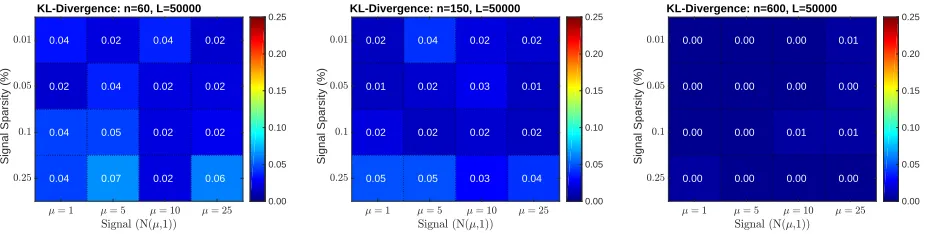
Figure 6 shows the KL-Divergence between the max null recovered by regular permutation testing and the max null recovered by RapidPT on 48 synthetically generated datasets (16
in each column). The input hyperparameters used were fixed to L = 50000, η = 2ηmin,
and l = n, where ηmin refers to the theoretical minimum sub-sampling rate and n is the
dataset size. As expected, the strength or sparsity of the signal does not have an impact on the performance of RapidPT. The dataset size, however, does have a slight impact on the
accuracy but we still find that the recoveredt-thresholds for the smaller datasets are within
KL-Divergence: n=60, L=50000
0.04
0.02
0.04
0.04 0.02
0.04
0.05
0.07 0.04
0.02
0.02
0.02 0.02
0.02
0.02
0.06
Signal Sparsity (%)
0.00 0.05 0.10 0.15 0.20
0.25 KL-Divergence: n=150, L=50000
0.02
0.01
0.02
0.05 0.04
0.02
0.02
0.05 0.02
0.03
0.02
0.03 0.02
0.01
0.02
0.04
Signal Sparsity (%)
0.00 0.05 0.10 0.15 0.20
0.25 KL-Divergence: n=600, L=50000
0.00
0.00
0.00
0.00 0.00
0.00
0.00
0.00 0.00
0.00
0.01
0.00 0.01
0.00
0.01
0.00
Signal Sparsity (%)
[image:22.612.70.533.72.189.2]0.00 0.05 0.10 0.15 0.20 0.25
Figure 6: KL-Divergence between the true max null and the one recovered by RapidPT on 48 datasets. The sub-sampling rate,η, used for each run was 2ηmin. The number of training samples,l, used for each run was n(i.e., the same as the number of images in the dataset).
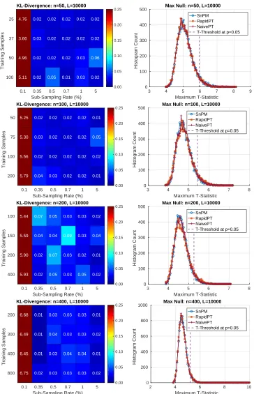
Results on the ADNI Dataset Can we recover the max null distribution?
The left column of Figure 7 uses a colormap to summarize the KL-Divergence results obtained from comparing the max null distributions of a single run of SnPM versus multiple RapidPT runs with various hyperparameters. The right column of Figure 7 puts the numbers displayed in the colormaps into context by showing the actual max null distributions for a single combination of hyperparameters. Each row corresponds to each of the four datasets used in our evaluations.
The sub-sampling rate was the hyperparameter that had the most significant impact on
the KL-Divergence. As shown in Figure 7, a sub-sampling rate of 0.1% led to high
KL-Divergence, i.e., the max null distribution was not recovered in this case. For every other
combination of hyperparameters RapidPT was able to sample at rates as low as 0.35% and
still recover an accurate max null distribution. Most KL-Divergence values were in the
0.01−0.05 range with some occasional values between 0.05−0.15. However, using the max
null distributions derived from only 2000 permutations leads to the resulting KL-Divergence
KL-Divergence: n=50, L=10000 4.76 3.66 4.96 5.11 0.02 0.03 0.02 0.02 0.02 0.02 0.02 0.05 0.02 0.02 0.02 0.01 0.02 0.02 0.03 0.03 0.02 0.02 0.06 0.02
0.1 0.35 0.5 0.7 1 5
Sub-Sampling Rate (%)
25 37 50 100 Training Samples 0.00 0.05 0.10 0.15 0.20 0.25
3 4 5 6 7 8 9
Maximum T-Statistic 0 100 200 300 400 500 Histogram Count
Max Null: n=50, L=10000
SnPM RapidPT NaivePT
T-Threshold at p=0.05
KL-Divergence: n=100, L=10000
5.25 5.30 5.56 5.79 0.02 0.03 0.02 0.04 0.02 0.02 0.02 0.03 0.02 0.02 0.02 0.02 0.02 0.02 0.02 0.02 0.01 0.05 0.02 0.01
0.1 0.35 0.5 0.7 1 5
Sub-Sampling Rate (%)
50 75 100 200 Training Samples 0.00 0.05 0.10 0.15 0.20 0.25
3 4 5 6 7 8
Maximum T-Statistic 0 100 200 300 400 500 Histogram Count
Max Null: n=100, L=10000
SnPM RapidPT NaivePT
T-Threshold at p=0.05
KL-Divergence: n=200, L=10000
5.44 5.59 5.90 5.93 0.07 0.04 0.02 0.02 0.05 0.04 0.07 0.05 0.03 0.09 0.03 0.03 0.03 0.03 0.02 0.05 0.02 0.04 0.01 0.02
0.1 0.35 0.5 0.7 1 5
Sub-Sampling Rate (%)
100 150 200 400 Training Samples 0.00 0.05 0.10 0.15 0.20 0.25
3 4 5 6 7 8
Maximum T-Statistic 0 100 200 300 400 500 Histogram Count
Max Null: n=200, L=10000
SnPM RapidPT NaivePT
T-Threshold at p=0.05
KL-Divergence: n=400, L=10000
6.68 6.49 6.45 6.75 0.01 0.01 0.01 0.02 0.03 0.04 0.03 0.03 0.03 0.03 0.04 0.03 0.03 0.03 0.04 0.03 0.01 0.02 0.01 0.02
0.1 0.35 0.5 0.7 1 5
Sub-Sampling Rate (%)
200 300 400 800 Training Samples 0.00 0.05 0.10 0.15 0.20 0.25
2 4 6 8 10
Maximum T-Statistic 0 200 400 600 800 1000 Histogram Count
Max Null: n=400, L=10000
SnPM RapidPT NaivePT
[image:23.612.118.482.69.634.2]T-Threshold at p=0.05
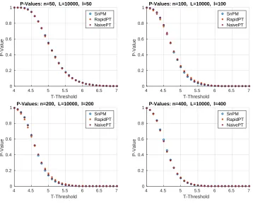
Are we rejecting the correct null hypotheses?
The test statistics obtained using the original data labels whose value exceed the t
-threshold associated to a givenp-value will correspond to the null hypothesis rejected. Figure
8 shows the resultant mapping betweent-threshold andp-values for the max null distribution
for a given set of hyperparameters. It is evident that the difference across methods is
minimal. Moreover, Figure 8 shows that lowp-values (p < 0.1), which are the main object of
interest, show the lowest differences. However, despite the low percent differences between
the p-values, in the larger datasets (100, 200, and 400 subjects) RapidPT consistently yields
slightly more conservative p-values near the tails of the distribution. Nonetheless, Figure 11
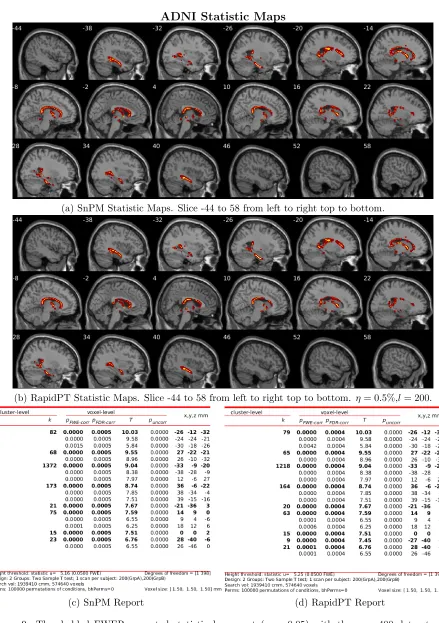
shows that the resampling risk between RapidPT and the two baselines remains very close to the resampling risk between both baselines. In practice, these plots show that RapidPT will reject the null hypothesis for a slightly lower number of voxels than SnPM or NaivePT. Despite the slight difference in thresholds, the actual brain regions whose null hypotheses were rejected consistently match between both methods as shown in Figures 9 and 10. Additionally, the regions picked up by both RapidPT and SnPM in Figure 9 correspond
to the Hippocampus – which is one of the primary structural brain imaging region that
corresponds to the signature of cognitive decay at the onset of Alzheimer’s disease. The regions in Figure 10 contain a subset of the brain regions in Figure 9 which is expected from the thresholds shown in the right column of Figure 7.
4 4.5 5 5.5 6 6.5 7
T-Threshold
0 0.2 0.4 0.6 0.8 1
P-Value
P-Values: n=50, L=10000, l=50
SnPM RapidPT NaivePT
4 4.5 5 5.5 6 6.5 7
T-Threshold
0 0.2 0.4 0.6 0.8 1
P-Value
P-Values: n=100, L=10000, l=100
SnPM RapidPT NaivePT
4 4.5 5 5.5 6 6.5 7
T-Threshold
0 0.2 0.4 0.6 0.8 1
P-Value
P-Values: n=200, L=10000, l=200
SnPM RapidPT NaivePT
4 4.5 5 5.5 6 6.5 7
T-Threshold
0 0.2 0.4 0.6 0.8 1
P-Value
P-Values: n=400, L=10000, l=400
[image:24.612.123.481.361.648.2]SnPM RapidPT NaivePT
ADNI Statistic Maps
(a) SnPM Statistic Maps. Slice -44 to 58 from left to right top to bottom.
(b) RapidPT Statistic Maps. Slice -44 to 58 from left to right top to bottom. η= 0.5%,l= 200.
[image:25.612.83.522.60.683.2](c) SnPM Report (d) RapidPT Report
ADNI Statistic Maps
(a) SnPM P-Map. Slice -44 to 58 from left to right top to bottom.
(b) RapidPT P-Map. Slice -44 to 58 from left to right top to bottom. η= 0.5%,l= 200.
[image:26.612.83.525.66.671.2](c) SnPM Report (d) RapidPT Report
Figure 10: Thresholded FWER corrected statistical maps at (α= 0.05) with the n = 200 dataset. The hyperparameters used were: η = 0.5%, l = n, and L = 100000. The images show the test statistics for which the null was rejected in SnPM (top) and RapidPT (bottom). The tables show a numerical summary of the images. The columns refer to: k - cluster size, pF W E−corr - corrected p-values, T - max cluster
0 0.02 0.04 0.06 0.08 0.1
P-Values
0 2 4 6 8 10
Resampling Risk (%)
Resampling Risk: n=200, L=10000, l=200
NaivePT-SnPM RapidPT-SnPM NaivePT-RapidPT
0 0.02 0.04 0.06 0.08 0.1
P-Values
0 0.5 1 1.5 2 2.5 3 3.5 4
Resampling Risk (%)
Resampling Risk: n=400, L=10000, l=400
[image:27.612.126.478.72.212.2]NaivePT-SnPM RapidPT-SnPM NaivePT-RapidPT
Figure 11: Resampling risk of NaivePT-SnPM, RapidPT-SnPM, and NaivePT-RapidPT. The hyperparam-eters used were: η= 0.35%,L= 10000, andl=n.
6.2. Runtime Performance
6.2.1. Effect of hyperparameters on the speed of RapidPT
Figures 12 and 13 show the speedup gains of RapidPT over SnPM and NaivePT, re-spectively. Each column corresponds to a single dataset, and each row corresponds to a different number of permutations. The supplementary results include an exhaustive version of these results that show the speedup gains of RapidPT for many additional number of permutations.
As shown in Figure 12, RapidPT outperforms SnPM in most scenarios. With the
excep-tion of theL= 2000 andL= 5000 runs on the larger datasets (n= 200 andn= 400), the
col-ormaps show that RapidPT is 1.5-30x faster than SnPM. As expected, a lowη (0.35%,0.5%)
and l (n2,3n4 ) leads to the best runtime performance without a noticeable accuracy tradeoff,
as can be seen also in Fig. 7 earlier.