Choosing among heterogeneous server clouds

warwick.ac.uk/lib-publications

Manuscript version: Author’s Accepted Manuscript

The version presented in WRAP is the author’s accepted manuscript and may differ from the

published version or Version of Record.

Persistent WRAP URL:

http://wrap.warwick.ac.uk/116202

How to cite:

Please refer to published version for the most recent bibliographic citation information.

If a published version is known of, the repository item page linked to above, will contain

details on accessing it.

Copyright and reuse:

The Warwick Research Archive Portal (WRAP) makes this work by researchers of the

University of Warwick available open access under the following conditions.

Copyright © and all moral rights to the version of the paper presented here belong to the

individual author(s) and/or other copyright owners. To the extent reasonable and

practicable the material made available in WRAP has been checked for eligibility before

being made available.

Copies of full items can be used for personal research or study, educational, or not-for-profit

purposes without prior permission or charge. Provided that the authors, title and full

bibliographic details are credited, a hyperlink and/or URL is given for the original metadata

page and the content is not changed in any way.

Publisher’s statement:

Please refer to the repository item page, publisher’s statement section, for further

information.

(will be inserted by the editor)

Choosing among heterogeneous server clouds

A. Karthik · Arpan Mukhopadhyay ·

Ravi R. Mazumdar

Received: date / Accepted: date

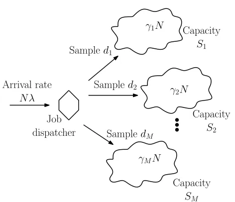
Abstract This paper considers a model of interest in cloud computing ap-plications. We consider a multi-server system consisting of N heterogeneous servers. The servers are categorized intoM(≪N ) different types according to their service capabilities. Jobs having specific resource requirements arrive at the system according to a Poisson process with rateN λ. Upon each arrival, a small number of servers is sampled uniformly at random from each server type. The job is then routed to the sampled server with maximum vacancy per server-capacity. If a job cannot obtain the required amount of resources from the server to which it is assigned, then the job is discarded. We analyze the system in the limit as N → ∞. This gives rise to a mean field, which we show has a unique fixed point and is globally attractive. Furthermore, as

N → ∞, the servers behave independently. The stationary tail probabilities of server occupancies are obtained from the stationary solution of the mean field. Numerical results suggest that the proposed scheme significantly reduces the average blocking probability compared to static schemes that probabilisti-cally route jobs to servers in proportion to the number of servers of each type. Moreover the reduction in blocking holds even for systems at high load. For the limiting system in statistical equilibrium, our simulation results indicate that the occupancy distribution is insensitive to the holding time distribution and only depends on its mean.

A. Karthik

E-mail: [email protected]

A. Mukhopadhyay

E-mail: [email protected]

Ravi R. Mazumdar

E-mail: [email protected]

Dept. of Electrical and Computer Engineering University of Waterloo

Keywords Heterogeneous servers · Multirate loss model · Mean field ·

Propagation of chaos

Mathematics Subject Classification (2000) MSC 60K35·MSC 90B15·

60J27· 60J80

1 Introduction

The cloud computing paradigm has found many applications ranging from data centers and web server farms to next generation wireless communication technologies such as cloud radio access network (C-RAN) [12]. Offloading jobs onto clouds allows users computational flexibility without the need to maintain resources themselves. Many infrastructure-as-service cloud computing systems are now commercially available such as Amazon EC2 [1], Google Cloud [3], Microsoft Azure [6], and IBM Cloud [5]. Such cloud service providers own and operate servers, and sell computational resources to their users in terms of virtual machines (VMs), which are blocks of resource instances such as CPU and memory.

A cloud facility typically consists of thousands of server machines, and hence VMs. A job may require multiple VMs on a particular server. Since a server has only a finite amount of resources, a job arriving at a server may be unable to obtain the required number of VMs for its processing. If the job is delay sensitive, the time to wait for a free resource might be prohibitive. In such a case, the job is blocked, or dropped, and cannot be processed. A prime objective for a cloud service provider, in order to ensure a certain grade of service, is to reduce the the probability that a job request is blocked.

In addition to this customer-centric goal, it is also in the self-interest of the cloud service provider to maximize the efficient use of all its resources. An important way to achieve this is to regulate and equally distribute incoming service requests among all its resources, referred to as load balancing. In fact, major commercial service providers of today such as Amazon EC2, Google Cloud, and Microsoft Azure do implement load balancing [2,4,7]. These com-mercial services implement load balancing at two different levels. First, by means of a high level user-controlled inferface, and second, at a lower level, user-independent internal implementation. Our study in this paper relates to the latter.

for a unit job might be smaller than that in cloud A. The primary dispatcher must therefore use this information for efficient job assignment to servers of different types.

It is well known that the blocking probability can be reduced by assigning arriving jobs to less congested servers [39,18,41]. Learning the states of all the servers before joining the least congested server, however, is infeasible due to the overhead incurred in such large systems. In such cases, randomized job assignment schemes offer practical alternatives [38,26,16]. In these schemes, a small, but random subset of server states is sampled and a job is assigned to the sampled server with the least occupancy. In models comprising of identical servers (homogeneous), randomly sampling just two servers and assigning a job to the server having the lower occupancy has been shown to drastically improve delay performance [38,26].

In this paper, we model the cloud system as a heterogeneous loss-system, which is motivated by the VM context, and consider a randomized scheme, referred to as maximum fractional vacancy (MFV) scheme, for job assignment. In this scheme, a small random subset of server states is sampled from each cloud. Jobs are then assigned to clouds whose sampled servers show the small-est occupancy per server-capacity.1 _{We then analyse the MFV scheme and}

study its system performance. The key contribution of this paper is to show that when the number of servers of each type is large we can exploit mean field theory to characterize the performance precisely, and show that propagation of chaos or independence of servers holds in the heterogeneous context too. Moreover we show that the blocking experienced by jobs using such a random-ized algorithm is very close to the lower bound on the blocking performance of such systems that can be achieved by any policy.

Randomized job assignment schemes have been primarily studied in the literature for a system consisting ofN identical first come first serve (FCFS) servers, which is also referred to as the supermarket model. Most studies con-sider the so called shortest-queue-d(SQ(d)) scheme in which each job is as-signed to the shortest ofd randomly chosen queues. Ford≥2, [38] showed, using the theory of operator semigroups, that the equilibrium queue sizes de-cay doubly exponentially in the limit as the system size increases (asN → ∞). Mitzenmacher in [26,27] derived the same result using an extension of Kurtz’s theorem [15]. Chaoticity on path space (or asymptotic independence among queue length processes) was established in [16] using empirical measures on the path space. The results of [38] were generalized to the case of open Jackson networks in [24].

The tradeoff between sampling cost of servers and the expected sojourn time seen by a customer in the supermarket model was studied under a game theoretic framework in [42]. Recently, in [30,29], the SQ(d) scheme was con-sidered for a system of parallel processor sharing servers with heterogeneous service rates. It was shown that, in the heterogeneous setting, random sam-pling ofdservers from the entire system reduces the stability region. However,

it can be recovered using the SQ(d) scheme over a randomly chosen server type.

Early works on mean field limits in routing problems in Erlang loss models include [23,8]. A large-system Erlang loss model for homogeneous servers was studied in [36]. It was shown here that the limiting system behaviour can be characterized using a system of differential equations. Simulation studies were used to show the super-exponential decay of the tail probabilities. Similar results were derived using an asymptotic independence ansatz in [31]. In [17], it was shown that loss models too exhibit propagation of chaos on the path space. Multi-server model for cloud systems with infinite waiting rooms, where jobs are queued till they obtain the required resources, was studied in the heavy traffic regime [22]. The assignment problem has also been in studied in the context of bin-packing problems under various constraints [34,9,25].

1.1 Main results

In this paper, we propose a new randomized scheme for job assignment in the heterogeneous scenario. In this scheme, upon arrival of a job, a small number of servers from each cloud is randomly sampled. The sampled servers are then compared based on their states and the arrival is assigned to the sampled server that has the highest vacancy per unit server-capacity.

This represents a scenario where a primary dispatcher first requests infor-mation from each cloud and then routes the job to the server that is likely to have the smallest blocking probability among the sampled servers. We an-alyze the performance of the proposed scheme in the limit as the system size

N → ∞using the mean field approach. Our analysis shows the following.

– The stationary tail distribution of server occupancies, in a system with a large number of servers, can be characterized by means of a fixed point of a system of differential equations (mean field limit).

– We establish the existence and uniqueness of the equilibrium point of the mean field equations in the space of empirical tail measures. Our proof dif-fers from the earlier works since closed form solutions cannot be obtained. – We show that propagation of chaos holds at each finite time and also at the equilibrium. In that, we generalize the earlier results on propagation of chaos to systems where exchangeability holds only among servers of the same type.

at each cluster of similar servers gives rise to blocking probabilities that are very close to the lower bound on blocking probabilities for such systems due to any policy, randomized or not, thus, showing the effectiveness and almost optimal behavior of such schemes.

1.2 Organization

The rest of the paper is organized as follows. In Section 2, we describe the system model, the MFV scheme, and our main result. We then analyze the MFV scheme using the mean field in Section 3. In Section 4, we generalize the model of Section 2 by introducing heterogeneous job classes, and show how stationary tail probabilities can be computed in this case, as well. In Section 5, numerical results are presented to benchmark the MFV scheme and to verify the accuracy of the theoretical results derived in the paper. Finally, we conclude the paper in Section 6 with a summary and a discussion on future work.

2 System model and main result

We consider a system comprising ofN parallel processing servers which are partitioned intoM(≪N) distinct types of server clouds. LetJ={1,2, . . . , M}

denote the index set of the cloud types, and letγjdenote the fraction of servers of typej. A cloud of typej∈ J containsγjN servers, each having the same finite capacity,Sj, of the total number of virtual machines (VMs). A job in a server of typej ∈ J engagesAj of the Sj available VMs at the server. The tuple (Sj, Aj) captures the resource and processing capabilities of a type j

server.

Jobs arrive at the system according to a Poisson process of rateN λ. Service times of jobs are exponentially distributed with a mean duration of 1/µunits.2

Further, service times are independent of one another, and also of the arrival process. Upon its arrival in the system, a job is routed to one of theN servers based on a routing scheme. If a server to which the job is routed has the required amount of resources to serve the job, then the processing of the job starts immediately. Otherwise, the job is discarded, or blocked. Resources used during the processing of a job are released upon its completion. We consider the following routing scheme in the rest of the paper, which we refer to as

maximum fractional vacancy scheme (MFV).

In this scheme, a job is routed to a server based on its occupancy, that is, the number of current jobs at the server. A local dispatcher at cloud j

samplesdj servers, uniformly at random, and conveys the smallest value,vj,

2 _{In this paper, we study the case of homogeneous job requests for which the assumption}

Job dispatcher

γ₁N

γ2N

γMN

Capacity S1

Capacity S2

Capacity SM

Sampled₁

Sampled₂

SampledM

Arrival rate N λ

Fig. 1 System consisting ofN parallel processor sharing (PS) servers, categorized intoM

types. There are γjN servers of type j, each of which has a capacity Sj. Arrivals occur according to a Poisson process with rateN λ. For each arrival, the job dispatcher samples

dj servers of typejand routes the arrival to one of the sampled servers.

of the sampled server occupancies thus found to the primary dispatcher.3_The

primary dispatcher then routes the job to the cloud that offers the smallest value ofvj/Cj for allj∈ J, where Cj is defined asCj = Sj

Aj. Ties are broken by preferring clouds with higher values of Cj. Without loss of generality, we suppose that

C1≤C2≤. . .≤CM. (1)

We observe that the number Cj is a measure of the total number of jobs that a type j server can simultaneously process. The scheme routes jobs to a sampled server having the least fractional occupancy, or equivalently, the highest fractional vacancy. This is illustrated in Figure 1.4_{We note that data}

models similar to the above have been employed in the research literature to address issues related to cloud services in various contexts [32,14,21,37].

3 _{For notational convenience, we assume that servers are sampled with replacement; the}

results in the paper remain unchanged even under the assumption that servers are sampled without replacement.

4 _{From an implementation viewpoint, each local dispatcherjmust periodically}

2.1 Main result

LetN_{denote the set of non-negative integers. For anyk∈}N_{andi, j∈ J, we}

define

⌊k⌋_ij = _Cj

Cik

+ 1, (2)

⌈k⌉_ij =

Cj Cik

, (3)

where ⌊x⌋ denotes the greatest integer not exceedingx and ⌈x⌉denotes the smallest integer greater than or equal tox. Define θj =⌊Cj⌋for j ∈ J. We are now ready to state the main result of the paper, which characterizes the system when the total number of servers is asymptotically large (N→ ∞).

Theorem 1 Let P_k(j)(N) denote the stationary probability that a server of type j has at least k unfinished jobs, in a system of N servers. Under the MFV scheme, P_k(j)(N) → P_k(j), as N → ∞, where for each j ∈ J, P_k(j) satisfies:

P_k(j₊₁) −P_k(₊₂j) = λ

µγj(k+ 1)

P_k(j)dj−P_k(j₊₁)dj

× j−1

Y

i=1

P_⌈(_ki)_⌉

ji

di _YM

i=j+1

P_⌊(_ki)_⌋

ji di

, for 0≤k≤θj−1, (4)

whereP0(j)= 1andP (j)

k = 0for k > θj.

Further, asN→ ∞, the stationary server occupancy distributions are inde-pendent. The blocking probability of the system is then given byQ

j∈J(P

(j) θj )

dj_.

The following sections of the paper are dedicated to deriving the above charac-terization. As we shall see in the analysis, (4) governs the state of the system under equilibrium, asN → ∞. Further, we show howP_k(j)can be easily com-puted. Thus, we can theoretically characterize and study the blocking proba-bility of the system. Since commercial cloud systems typically contain a large number of servers, asymptotic analysis (N → ∞) is natural and relevant for such systems. Moreover, we note that since arrivals at a given server depend on the states (occupancies) of other servers, obtaining the exact time evolution of the system is difficult. Large system analysis also aids analytical tractablility. The limiting system behaviour is known as the mean field limit [26,38,24].

3 The mean field

3.1 Notation

We define the following real sequence spaces:

UN,θj={{gn}_n∈N: 1 =g0≥g1≥. . .≥gθj, gn= 0 forn > θj, γjgnN ∈N},

(5)

Uθj ={{gn}n∈N: 1 =g0≥g1≥. . .≥gθj, gn = 0 forn > θj}. (6)

Let UN = Q

j∈J UN,θj and U = Q

j∈J Uθj denote the Cartesian products of

UN,θj and Uθj, respectively, over j ∈ J. For u,v ∈ U, define the distance between them as

ku−vk= sup

j∈J

sup

n∈N

u(nj)−v(nj) n+ 1

. (7)

Note thatU is closed under the above metric, bounded, and finite-dimensional. Hence, under the metric defined in (7), the space U is compact (and hence complete and separable).

Let (H,H, µH) be a measure space and f : H → R _{be a µH-integrable}

function. We define duality brackets ashf, µHi=R

f dµH. We denote the weak convergence (convergence in distribution) of a sequence of probability measures

Pn (random variablesXn) to a probability measure P (random variable X) byPn ⇒P (Xn ⇒X).

Let x,x′_{,y ∈ U. We denote x ≤ x}′ _{to mean x}(j) k ≤ x′

(j)

k for all j ∈ J

and k ∈ N_{. Further, y = min(x,x}′_{) and y = max(x,x}′_{) means that y}(j)

k =

min(x(_kj), x′(j)

k ) and y (j)

k = max(x (j) k , x′

(j)

k ), respectively, for all j ∈ J and k∈N_.

3.2 Analysis

We define the process

xN(t) =

n

x(_N,nj) (t), j∈ J, n∈No _{fort≥0, (8)}

wherex(_N,nj) (t) denotes the fraction of typejservers having at leastnunfinished

jobs at time t. Thus nx_N,n(j) (t), n∈No _{denotes the empirical tail distribution}

of occupancy of type j servers at time t. Observe that xN(t) ∈ UN. In the

following lemma, we evaluate the generator AN associated with the process

xN(t).

AN of the Markov processxN(t)acting on functionsf :UN →Ris given by

ANf(g) =N λ M

X

j=1 θj X

n=1

gn(j−)1

dj

−g(nj)

djj_Y−1

i=1

g_⌈(i_n)_−1⌉

ji di

× M

Y

i=j+1

g_⌊(i_n)_−1⌋

ji di

f(g+e(n, j)

N γj )−f(g)

+µN M

X

j=1 θj X

n=1

γjng(j) n −g

(j) n+1

f(g−e(n, j)

N γj )−f(g)

. (9)

Proof The proof is given in Appendix A.

We now state the main result of this section, which essentially captures the asymptotic behaviour ofxN(t), asN → ∞. In particular, we employ the

generator AN to show that the process xN(t) converges to a deterministic

process asN → ∞.

Theorem 2 If xN(0) converges in distribution to some constant g ∈ U as N → ∞, then the process {xN(t)}t≥0 converges in distribution to a process {u(t)}_t≥0, lying in the space U as N → ∞. The process u(t) is given by the solution of the following system of differential equations

u(0) =g, (10)

˙

u(t) =l(u(t)), (11)

where the mappingl:U → RNM is given by

l_k(j)(u) = 0, for k= 0 andk > θj, j∈ J, (12)

l_k(j)(u) = λ

γj

u(_kj−)1

dj

−u(_kj)dj

j−1 Y

i=1

u(_⌈i_k)_−1⌉

ji

di _YM

i=j+1

u(_⌊i_k)_−1⌋

ji di

−kµu(_kj)−u_k(j₊₁) , for 1≤k≤θj, j∈ J. (13)

The process {u(t)}_t≥0, defined in the theorem above, is referred to as the

mean field. We first note that Theorem 2 implicitly assumes that the ordinary differential system (10)-(11) has a unique solution in the space U. In the fol-lowing proposition, we show that this is indeed the case. To emphasize the dependence of the solution u(t) on the initial point g, we will often denote u(t) byu(t,g).

Proposition 1 If g ∈ U, then the system (10)-(11) has a unique solution

u(t,g)∈ U, for allt≥0.

We will prove Theorem 2 using the theory of semigroup operators of Markov processes as in [38,24]. First, we recall the following from [15].

– For the process{xN(t)}t≥0, the operator semigroup{TN(t)}t≥0 acting on

continuous functions f :UN →R_{is defined as}

TN(t)f(x) =E[f(xN(t))|xN(0) =x] ∀t≥0,x∈ UN.

– For the deterministic process{u(t)}_t≥0, the transition semigroup{T(t)}t≥0

acting on continuous functionsf :U →R_{is defined as}

T(t)f(x) =f(u(t,x)) ∀t≥0,x∈ U.

In the next proposition, we show thatTN(t) converges toT(t) uniformly

on bounded intervals. This in conjunction with Theorem 2.11 of Chapter 4 of [15] proves Theorem 2.

Proposition 2 Let u(t,g) be the solution to the system (10)-(11). For any continuous functionf :U →Randt≥0,

lim

N→∞_gsup_∈UN|TN(t)f(g)−f(u(t,g))|= 0, (14)

and the convergence is uniform int within any bounded interval.

Proof The proof is given in Appendix C.

Remark 1 We note that Theorem 2 implies that ifxN(0)⇒g∈ UN as N → ∞, then the following weaker convergence results also hold:

1. For eacht≥0,xN(t)⇒u(t,g) asN → ∞.

2. For eacht≥0,j∈ J, andk∈N_,x(j)

N,k(t)⇒u (j)

k (t,g) asN → ∞.

3. For eacht≥0,j∈ J, andk∈N_,Eh_x(j)

N,k(t)

i

→u(_kj)(t,g) asN → ∞.

The last assertion follows from the first since x(_N,kj)(t) is bounded for each

N, j, k, t.

3.3 Properties of the mean field

In this section, we characterize some important properties of the mean field. In particular, we show that (10)-(11) has a unique globally asymptotically stable equilibrium point inU.

LetPdenote an equilibrium point of (10)-(11). Then,Psatisfiesl(P) =0. The following proposition guarantees that there exists an equilibrium point of the system (10)-(11)U.

xN(t) u(t)

xN(∞) P

t→ ∞

N→ ∞

Theorem 2

N→ ∞

Theorem 5

t→ ∞

T

h

eo

re

m

4

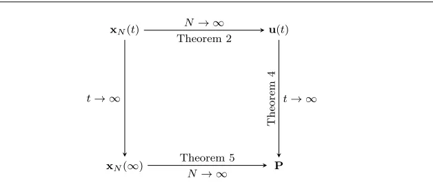
Fig. 2 Commutativity of limits

Proof The proof is given in Appendix D.

The next theorem shows thatPis the unique globally asymptotically stable equilibrium point of the system (10)-(11) in the spaceU.

Theorem 4

lim

t→∞u(t,g) =P∈ U for all g∈ U, (15)

Hence, P is a globally asymptotically stable fixed point of systems (10)-(11). Furthermore,Pis the only equilibrium point of the above systems in the space U.

Proof The proof is given in Appendix E.

We now show that the stationary distribution of the process xN(t)

con-verges weakly to the Dirac measure concentrated at the unique equilibrium point of the mean field. LetπN denote the stationary distribution of the pro-cessxN(t). SincexN(t) is positive recurrent,πN exists and is unique.

Theorem 5 We have

πN ⇒δP, asN → ∞. (16)

Proof The proof is given in Appendix F.

For each fixedN, letxN(∞) be a random variable distributed asπN. By

ergod-icity, we havexN(t)⇒xN(∞) ast→ ∞. We have so far established that the

interchange property indicated in Figure 2 holds. Note that the convergences indicated in the figure are in distribution.

We observe the following simple upper bounds onP_θ(_jj).

Proposition 3 Let τj = λ

µγj. Whendj ≥2 for each j∈ J,

P_θ(_jj)≤ τ

dθj_j −⌈τj⌉+1−1

dj−1 j

Qθj−⌈τj⌉

k=0 (θj−k) dk

j

Whendj= 1 for eachj ∈ J,

P_θ(_jj)≤ τ

θj−⌈τj⌉+1

j

Qθj−⌈τj⌉

k=0 (θj−k)

. (18)

Proof The proof is given in Appendix G.

Thus, we infer that when at least two servers are sampled from each server type, the tail blocking probabilityQ

j∈J(P

(j) θj )

dj _{decays at a much faster rate}

than when a single server is sampled from each cloud. This behaviour is com-mon in power-of-two randomized schemes [38,26,27].

3.4 Propagation of chaos

In this subsection, we focus on the occupancies of a given finite set of servers as N → ∞. We show that as the system size grows the server occupancies become independent of each other. Such independence holds at any finite time and also at the equilibrium, provided that the initial server occupancies satisfy certain assumptions. This is formally known as the propagation of chaos[16, 35] orasymptotic independence property [11,10] in the literature.

To formally state the results we introduce the following notations. Let

q(_Nj,k)(t), for j ∈ J and k ∈ {1,2, . . . , N γj}, denote the occupancy of the

kth _{server of type j at time t ≥ 0. By q}(j,k)

N (∞) we denote the occupancy

of the kth _{server of type j in equilibrium. Further, let χ}(j)

N,n(t), for j ∈ J

andn∈N_{, denote the fraction of typej servers having occupancynat time}

t≥0. Define the processχ_N(t) =

n

χ(_N,nj) (t), j∈ J, n∈No_{. Clearly,χ}(j)

N (t) =

n

χ(_N,nj) (t), n∈No_{denotes the empirical distribution of occupancies of type j}

servers and for eachn, j, we haveχ(_N,nj) (t) =x(_N,nj) (t)−x(_N,j)_(n+1)(t). Byχ(_Nj)(∞) we will denote the empirical distribution occupancies for type j servers in equilibrium. Let the process Q(t) = nQn(j)(t), j∈ J, n∈N

o

be defined as

Qn(j)(t) = u(nj)(t)−un(j+1) (t), for t ∈ [0,∞]. Further, we denote by Q(j)(t)

the distribution on N _{given by Q}(j)_{(t) =} n_Q(_nj)_{, n∈}No_{. We also define the}

following notion of exchangeable random variables.

Definition 1 Letnq(_Nj,k),1≤k≤N γj,1≤j≤Modenote a collection ofN

random variables among which N γj belong to a particular class j and are indexed by k, where 1 ≤ k ≤ N γj. The collection is called intra-class ex-changeable if the joint law of the collection is invariant under permutation of indices, 1≤k≤N γj, of random variables belonging to the same class.

1. For each fixkandt∈[0,∞],q_N(j,k)(t)⇒U(j)_{(t)asN → ∞, where U}(j)_(t) is a random variable with distribution Q(j)_(t).

2. Fix positive integersr1, r2, . . . , rM. For each t∈[0,∞],

n

q_N(j,k),1≤k≤rj,1≤j≤Mo⇒nU(j,k)_{(t),1≤k≤rj,1≤j≤M}o_,

as N → ∞, where U(j,k)_{(t), 1 ≤ k ≤ rj,1 ≤ j ≤ M, are independent} random variables with U(j,k)_{(t)having distributionQ}(j)_{(t)for all1≤k≤} rj.

Proof The proof is given in Appendix H.

Thus, the above proposition shows that in the limiting system server oc-cupancies become independent of each other. It also shows that the sta-tionary occupancy distribution of any type j server is given by Q(j)_{(∞) =}

n

Pn(j)−Pn(j+1) , n∈N

o .

Remark 2 Since the server occupancies are asymptotically independent, the arrival process of jobs at any server in the limiting system is a state dependent Poisson process. The arrival rate of jobs at a server of typej ∈ J, when its occupancy is k is given by (31) given in Appendix D. This equation can be explained as follows.

Consider a tagged typej server in the system and the arrivals that have the tagged server as one of its possible destinations. These arrivals constitute the potential arrival process at the tagged server. The probability that the tagged server is selected as a potential destination server for a new arrival is N γj−1

dj−1

/ N γj

dj

= dj

N γj. Thus, due to Poisson thinning, the potential arrival process to the tagged server is a Poisson process with ratedj/N γj×N λ=djλ

γj . Consider the potential arrivals at the tagged server when its occupancy is k. This arrival actually joins the tagged server with probability _x+11 when

xother servers among the dj servers of typej have occupancy k, all the di

servers of type i < j have at least occupancy⌈k⌉_ij, and all the di servers of typei > j have at least occupancy⌊k⌋_ij. Thus, the total arrival rateλ(_kj) can be computed as

λ(_kj)= djλ

γj dj−1

X

x=0

1

x+ 1

_dj−1

x

P_k(j)−P_k(+1j)

x

P_k(+1j)

dj−1−x

× j−1

Y

i=1

P_⌈(_ki)_⌉

ij

di _YM

i=j+1

P_⌊(_ki)_⌋

ij di

, (19)

which simplifies to (31).

can in turn be expressed as functions of the arrival rate. Indeed, we note that (33) in Appendix D expresses the local balance equations in equilibrium, which hold under state dependent Poisson arrivals due to Theorems 3.10 and 3.14 of [20].

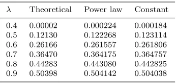
Remark 3 So far our results have been obtained for exponential job length distributions. Under the hypothesis that asymptotic independence is observed in stationarity even under general job length distributions, the blocking prob-ability of the system seems to depend only on the mean of the job length distribution (insensitivity). In [11] they conjecture that asymptotic indepen-dence holds for any local service discipline (rates only depend on current jobs in service) under general service time distributions. This would then imply that the arrivals to individual queues are state dependent Poisson processes that depend only on the state of that queue. This together with the result of Zachary [43] would then imply that insensitivity holds. However lacking a proof of asymptotic independence in the general service time case we can only claim insensitivity as a conjecture.In Section 5, we provide numerical evidence to support this hypothesis.

4 Heterogeneous jobs model

In this section, we relax the assumption that jobs have the same mean dura-tion. This is a more realistic model for jobs; for example, some jobs might be computationally more intensive than other jobs and hence might have higher mean durations. We assume here that a job may belong to one ofLtypes. Let

L={1, . . . , L} denote the class of job-types. A job of typel ∈ Lhas a mean duration of 1/µlunits. A job of typel∈ L, in a server of typej∈ J engages

A(_lj) of the Sj available VMs at the server. The tuple (Sj, A(_lj)) captures the resource and processing capabilities of a type j server with respect to a job of type l ∈ L. Further, we assume that jobs of type l ∈ L arrive indepen-dently at the system according to a Poisson process of rate N λl. Note that the MFV scheme still compares the fractional total occupancies of servers for job assignment.

eachj∈ J:

X

l∈L

λl γjµl

p(j)_k−A(j) l

dj

−p(j)_{k+ 1−A}(j) l

dj

× j−1

Y

i=1

p(i)l_k−A(j) l

m

ji

di M Y

i=j+1

p(i)j_k−A(j) l

k

ji

di

=k(p(j)_(k)−p(j)_{(k+ 1)),0≤k≤Sj, (20)}

where p(j)_{(k) = 1 for k ≤ 0, and p}(j)_{(k) = 0 for k > Sj. From this, the}

blocking probabilityPb(,lj) of a job of type l ∈ L at a server of typej ∈ J is

given byp(j)_Sj−A(j) l + 1

, and the system blocking probability of a typel

job is thus calculated asQ

j∈J

P_b(_,lj)dj.

5 Numerical results

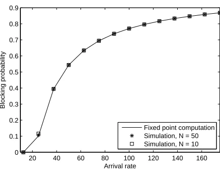
We first present simulation results that verify the asymptotic analysis pre-sented in the paper. In Figure 3, we plot the average blocking probability of the system as a function of the arrival rateλ forN = 50 and N = 10. Also shown is the blocking probability computed as Q

j∈J(P

(j) θj )

dj_{, where P}(j)

θj is obtained as the solution to the fixed point equation (4). Specifically, the unique fixed pointPwas computed by a repeated application of the map presented in Appendix D. For the simulation set up, we considerθ1= 20,θ2= 25,A1= 2, A2 = 3, 1/µ= 1,γ1=γ2 = 0.5, andd1 =d2= 2. We note the match of the

results from the fixed point analysis with the simulations for both the values ofN. This supports the approach of asymptotic analysis, via the mean field, that we have employed in the paper, and provides a theoretical alternative to characterize the system blocking.

Next, we compare dependent job assignment schemes with state-independent job assignment schemes. In Figure 4, we plot the average blocking probability, as a function of the normalized arrival rate, seen by the system under the MFV scheme, which is state-dependent, and two state-independent schemes referred to as static routing-1 and static routing-2, in which jobs are routed to clouds with fixed probabilities. For the set up, we considerN= 50,

θ1 = 20,θ2 = 25,A1= 2, A2= 3, 1/µ= 1,γ1=γ2 = 0.5, andd1=d2 = 2.

In the static routing-1 scheme, a job is assigned to a cloudj with probability

γjθj/(P

i∈J γiθi). Note that this scheme is independent of the arrival rateλ.

20 40 60 80 100 120 140 160 0

0.1 0.2 0.3 0.4 0.5 0.6 0.7 0.8 0.9

Arrival rate

Blocking probability

Fixed point computation Simulation, N = 50 Simulation, N = 10

Fig. 3 Blocking probability as a function of the arrival rate.

at the normalized arrival rate of 0.5. This shows the advantages of simple, ran-domized state-dependent job assignment schemes over the state-independent ones.

Also shown in Figure 4 is a theoretical lower bound on the system blocking probabilityPbof any job assignment scheme, which is obtained by the following

argument. The effective arrival rate of jobs at the system equalsN λ(1−Pb),

and by Little’s law, the average number of jobs in the system is given by

N λ(1−Pb)/µ=P_j∈JN γj

Pθj

k=1P (j) k ≤

P

j∈J N γjθj. Thus, we have Pb ≥

max{0,1−µ P

j∈Jγjθj

λ }. We denoteλc =µ

P

j∈Jγjθj as the critical arrival

rate. It is the largest arrival rate at with the lower bound evaluates to 0. We observe from the figure that the MFV scheme has a system blocking probability that is very close to the theoretical lower bound, which hints that the MFV scheme is very close to optimal. We explore this further in Figure 5 and Figure 6 for two different system settings having γ1 =γ2 = 0.5 and d1 =d2 = 2. We

observe that in both cases, the margin between the simulation values and the corresponding lower bounds is not greater than 10%. Thus, the MFV scheme closely follows the optimal assignment scheme.

In Figure 7, we consider a system of N = 100 servers such that θ1 = 20, θ2 = 40, and µ = 1/3. We plot the blocking probability for two different

sampling configurations as a function of the arrival rate near the region of critical arrival rate, which in this case is λc = 10. We observe from the plot that more number of samples yields smaller blocking probabilities. This is because of the greater chance of choosing a shorter queue, when more than one server is sampled.

0.5 1 1.5 2 2.5 3 3.5 0

0.1 0.2 0.3 0.4 0.5 0.6 0.7 0.8 0.9 1

Normalized arrival rate

Blocking probability

Static routing−1 MFV scheme Lower bound Static routing−2

Fig. 4 Blocking probability as a function of the normalized arrival rate.

10 15 20 25 30 35 40

0 0.05 0.1 0.15 0.2 0.25 0.3 0.35 0.4 0.45 0.5

Arrival rate

Blocking probability

Lower bound Simulation

Fig. 5 Comparison with lower bound in the under-loaded regime.N= 50,θ1= 25,θ2= 20.

Table 1 Insensitivity of MFV scheme

λ Theoretical Power law Constant

0 5 10 15 20 25 30 0

0.1 0.2 0.3 0.4 0.5 0.6 0.7

Arrival rate

Blocking probability

Lower bound Simulation

Fig. 6 Comparison with lower bound in the under-loaded regime.N= 100,θ1= 5,θ2= 20.

9 9.5 10 10.5 11

0 0.02 0.04 0.06 0.08 0.1 0.12 0.14

Arrival rate

Blocking probability

d₁ = d₂ = 1 d₁ = d₂ = 2

Fig. 7 Comparison with different sampling numbers.N= 100,θ1= 20,θ2= 40,µ= 1/3.

1. Constant: We consider job length distribution having the cumulative dis-tribution given byF(x) = 0 for 0≤x <1/µ, andF(x) = 1, otherwise. 2. Power law: We consider job length distribution having cumulative

distri-bution function given byF(x) = 1−1/4µ2_x2 _forx≥ 1

2µ and F(x) = 0,

otherwise.

6 Conclusions

In this paper, we analyzed the MFV scheme for a heterogeneous multi-server Erlang loss system. We showed that in the large system limit the evolution of the empirical occupancy distribution can be characterized through its mean field limit. We established the existence and uniqueness of the stationary point of the mean field limit. Furthermore, we showed that propagation of chaos holds for heterogeneous case through the requirement of type-based exchange-ability. The foregoing results were shown for the exponential job length distri-bution. An interesting avenue to explore is if these can be replicated for generic job length distributions, as well. Our numerical results hint that asymptotic independence is exhibited even under generic job length distributions.

Further, we observed that the MFV scheme is very nearly optimal in per-formance. This shows the effectiveness of such simple randomized assignment schemes. We remark that similar state dependent assignment schemes, for in-stance, assigning to servers with smallest vacancy, or least occupancy, must have similar system behaviour.

A Proof of Lemma 1

We recall the generatorAN of the semigroup{TN(t)}t≥0 acting on functionsf:UN→R is given by ANf(g) =

P

h6=gqgh(f(h)−f(g)), where qgh, withg,h ∈ UN, denotes the transition rate from stategto stateh[15].

Consider an arrival at timetthat joins a server of typejwith exactlyn−1 unfinished jobs, when the state of the system isg. This corresponds to the transition from stategto the stateg+e_{N γ}(n,j)

j since the fraction of typejservers with at leastnunfinished jobs increases by 1/N γj, whereas the empirical tail occupancies of the other servers remain unchanged. This transition occurs in the MFV scheme only when the following conditions are satisfied:

– Among the dj sampled servers of typej, at least one has exactly n−1 jobs and the rest of them have at leastnjobs. Since there areN γjgn(j−)1andN γjg(nj) servers with at least n−1 andnjobs, respectively, uniform sampling of the typej servers result in a

probability of (N γjg

(j)

n−1)dj−(N γjg(nj))dj

(N γj)dj

= (g(nj−)1)dj −(g (j)

n )dj for this case.

– For eachi < j, all thedisampled servers of typeihave fractional occupancies satisfying

i/Ci≥(n−1)/Cj; equivalently, sampled servers of typeimust have at least⌈n−1⌉ji jobs. Proceeding as above, the probability of this case isQj−1

i=1(g (i)

⌈n−1⌉_ji)di.

– For eachi > j, all thediservers of typeihave fractional occupancies satisfyingi/Ci> (n−1)/Cj; equivalently, sampled servers of type imust have at least ⌊n−1⌋ji jobs. The probability of this case is then calculated asQM

i=j+1(g (i)

⌊n−1⌋_ji)di.

Thus, the probability with which an arrival joins a type j server with exactlyn−1 jobs

is given by

g_n(j₋)₁dj −g(nj)

djQj−1

i=1

g_⌈(i_n)_−1⌉

ji

di

QM i=j+1

g_⌊(i_n)_−1⌋

ji

di

. Since the

arrival rate of jobs isN λ, the rate of the above transition is given by

q

g,g+e(n,j)

N γj =N λ

g(nj−)1

dj

−g(nj)

djjY−1

i=1

g(_⌈i_n)_−1⌉

ji

di _YM

i=j+1

g(_⌊i_n)_−1⌋

ji

di

.

Finally, the rate at which jobs depart from a server of type j having exactly n jobs is

µnN γj

g(nj)−gn(j+1)

e(n,j)

N γ_j since the fraction of type j servers with at least n unfinished jobs decreases by 1/N γj, whereas the empirical tail occupancies of the other servers remain unchanged. The expression (9) now follows from the definition ofAN.

Remark 4 We observe that the foregoing expressions are obtained under the assumption that thedj, j∈ J servers are sampled with replacement. If, however, they were sampled without replacement, the probability of each of the aforementioned cases changes as follows.

– Servers of the tagged typej: The probability that at least one of them has exactlyn−1

jobs and the rest of them have at leastnjobs becomes

N γjg(nj−)1

dj

− N γjg(nj) dj

/ N γj dj

.

– Servers of type i < j: The probability that each of them has⌈n−1⌉jijobs at least is

given byQj−1

i=1

N γig(⌈in)−1⌉_ji di

/ N γi

di

.

– Servers of typei > j: The probability that each of them has⌊n−1⌋jijobs at least is

given byQj−1

i=1

N γig(⌊in)−1⌋_ji di

/ N γi

di

.

Consequently, we obtain a different form for the generator ofxN(t), sayA′N.5 We note that in the limit asN→ ∞, the probabilities in each of the above cases reduce, respectively, to exactly those obtained when servers are sampled with replacement. This fact when used in a parallel development leading up to (30) shows limN→∞A′Nf(g) = _dtdf(u(t,g))|t=0.

Hence, even when servers are sampled without replacement, the same mean field, as in the case of sampling with replacement, is obtained. We consider the latter case for the analysis of MFV for ease of notation; it leads to no change in any of the asymptotic results presented in the paper.

B Proof of Proposition 1

Defineφ:R_{→[0,1] as φ(x) = [min{x,1}]+, where [z]+ = max{0, z} and consider the} following modification of the system (10)-(11):

u(0) =g, (21)

˙

u(t) =ˆ_{l(u(t)), (22)}

where the mappingˆl: RNM

→ RNM

is given by

ˆ

l(kj)(u) = 0 fork= 0 andk > θj, j∈ J, (23)

ˆ

l(_kj)(u) = λ

γj

φ(u(_kj₋)₁)dj−φ(u(_kj))dj

+

j−1

Y

i=1

φ(u(_⌈i_k)_−1⌉

ji)

di _YM

i=j+1

φ(u(_⌊i_k)_−1⌋

ji)

di

−kµhφ(u(_kj))−φ(u(_kj₊₁) )i

+, for 1≤k≤θj, j∈ J. (24)

5 _{In fact, forf:U}

N→R,

A′Nf(g) =N λ

M X j=1 θj X n=1

N γ_jg(_nj₋)₁ dj

− N γjgn(j) dj

N γj dj

j−1

Y

i=1

N γ_ig(i) ⌈n−1⌉_ji

di

N γi di

j−1

Y

i=1

N γ_ig(i) ⌊n−1⌋_ji

di

N γi di

×

f(g+e(n, j)

N γj

)−f(g)

+µN M X j=1 θj X n=1

γjn

gn(j)−g(nj+1)

f(g−e(n, j) N γj

)−f(g)

Clearly, the right hand side of (11) and (24) are equal ifu∈ U. Therefore, the two systems must have identical solutions inU. Also ifg∈ U, then any solution of the modified system remains withinU. This is because of the facts that ifu(nj)(t) = u(nj+1) (t) for some

j,n,tin (24) then ˆln(j)(u(t))≥0 and ˆl( j)

n+1(u(t))≤0, and ifu (j)

n (t) = 0 for somej,n,t, then ˆl(nj)(u(t))≥0. Hence, to prove the uniqueness of solution of (10)-(11), we need to show that the modified system (21)-(22) has a unique solution in (RZ+₎M_{. We now extend the}

distance metric defined in (7) to the space (RN )M_.

Using the metric defined in (7) and the facts that|x+−y+| ≤ |x−y|for anyx, y∈R,

a₁bm₁ −a₂bm₂

≤ |a₁−a₂|+m|b₁−b₂|for anya₁, a₂, b₁, b₂∈ [0,1], and|φ(x)−φ(y)| ≤ |x−y|for anyx, y∈R_{we obtain}

kˆl(u)k ≤K1, (25)

kˆ_l(u)−ˆ_{l(w)k ≤K2ku−wk, (26)}

where u,w∈ (RN₎M_{,K1 and K2 are constants defined asK1 =} λ

minj∈Jγj +µθM and

K2= 4M λmaxj∈J

dj

minj∈Jγj + 3µθM. The uniqueness now follows from inequalities (25) and (26) by using Picard’s iteration technique since (RN₎M _{is complete under the metric defined}

in (7). ⊓⊔

C Proof of Proposition 2

We prove Proposition 2 by showing that the generatorsANof the corresponding semigroups converge asN→ ∞to the generatorAof the deterministic processu(t,g).

First, we show that the solutionu(t,g) of (10)-(11) is smooth with respect to the initial pointgand its partial derivatives are bounded.

Lemma 2 Letu(t,g) denote the solution of (10)-(11). For each j,n, j′, n′, i, k, and

t≥0, the partial derivatives ∂u(t,g)

∂g(_nj) , ∂2u(t,g)

∂gn(j)

2 , and

∂2u(t,g)

∂g(nj)∂g(j ′)

n′

exist forg∈ U and satisfy

∂u(_ki)(t,g)

∂g(nj)

≤exp(B1t) (27)

and

∂2_u(i)

k (t,g)

∂gn(j)

2 ,

∂2_u(i)

k (t,g)

∂g(nj)∂g(j ′₎ n′

≤B2 B1

(exp(2B1t)−exp(B1t)), (28)

whereB1=2

λmaxj∈Jdj

minj∈Jγj + 2µθM maxj∈J

, andB2=2

λ(maxj∈Jdj)2

minj∈Jγj .

Proof The proof follows the same line of arguments as the proof of Lemma 3.2 of [24]. Fix

j,n,g and defineu′(t) =∂u(t,g)/∂g(nj). If this partial derivative exists, thenu′(t) must satisfyu′(i)

0 (t) = 0,u′ (i)

k (0) =δijδkn. Further, by differentiating (13) we obtain (variable t is supressed for simplifying notation)

du′(i)

k dt = λ γj di

u(_ki₋)₁di−1u′(_ki₋)₁−u(_ki)di−1u′(_ki) i−1

Y

l=1

u(_⌈l_k)_−1⌉

il

d_l

×

M

Y

l=i+1

u(_⌊l_k)_−1⌋

il

d_l

−µku′(ki)−u′

(i)

k+1

Conversely, ifu′(t) is a solution of the system above, then it must be the required partial derivative. Using Lemma 3.1 of [24] witha=B,b0= 0, andc= 1 and the fact that

u

(k)

r

≤1 for allk,rit can be shown that

∂u(rk)(t,g) ∂g(nj)

exists and is bounded as given by (27).

Similarly, by differentiating (29) again with respect tog(nj) andg(j ′₎

n′ , we get the system of equations in ∂2u

(k)

r (t,g) ∂gn(j)

2 and

∂2u(rk)(t,g) ∂g(nj)∂g(j

′)

n′

, respectively. Lemma 3.1 of [24] can be applied

again to this system to show that the second order partial derivatives also exist and are bounded as given by (28).

Next, we show convergence of the generatorsAN. Note that the following arguments are along the same lines of the proof of Theorem 2 in [24]. We repeat them here for completeness. LetLdenote the set of real continuous functions onU, and letDdenote the set off∈L

such that the partial derivatives∂f(g) ∂gn(j)

,∂2f(g) ∂g(nj)

2, and

∂2f(g)

∂g(nj)∂g(j ′)

n′

exist for allg, j, j′_{, n, n}′_{, and}

are uniformly bounded. Using the norm (7) onU and the sup-norm onL, we note thatD

is dense inL. Further, forf∈D, we have

N

f(g+e(n, j)

N γj

)−f(g)

→ 1

γj

∂f(g)

∂gj(n)

,

N γj

f(g−e(n, j) N γj

)−f(g)

→ −∂f(g) ∂gj(n)

,

uniformly ing∈ U, which upon substitution in (9) of Lemma 1 yields

lim

N→∞ANf(g)

= M X j=1 θj X n=1

∂f(g)

∂gj(n)

λ γj

gn(j−)1

dj

−g(nj)

dj j−1

Y

i=1

g(_⌈i_n)_−1⌉

ji

d_i M Y

i=j+1

g_⌊(i_n)_−1⌋

ji d_i − M X j=1 θj X n=1

∂f(g)

∂gj(n)

µng(nj)−g( j) n+1 , = M X j=1 θj X n=1

∂f(g)

∂gj(n)

       λ γj

g(nj−)1

d_j −gn(j)

d_jjY−1

i=1

g(_⌈i_n)_−1⌉

ji

di _YM

i=j+1

g(_⌊i_n)_−1⌋

ji

di

−µng(nj)−gn(j+1)

     , = d

dtf(u(t,g)) t=0 , (30)

uniformly ing∈ U.

We define a semigroup of operatorsT(t), t≥0 inLby settingT(t)f(g) =f(u(t,g)). Observe that the generatorAof this semigroup is given byAf(g) = limt↓0T(t)f(gt)−f(g)=

d

dtf(u(t,g))|t=0, which coincides with the RHS of (30).6 Thus, we obtainANf →Af, in the sup norm for allf∈D.

Next, defineD0 ⊂D as those funcitons inD that depend on finitely many variables

gj(n). By the norm defined in (7) we note thatD0is dense inD, and hence inL. Further, by

Lemma 2,f0∈D0 =⇒ T(f0)∈D. In addition, we note that the corresponding semigroups TN(t) andT(t) are continuous and contracting in the space of continuous real functions on

U. These facts, along with Proposition 3.3 and Theorem 6.1 of [15] gives the desired result.

6 _{Recall that the generatorAof the semigroup{T(t)}}

t≥0acting on functionsf:U →R

D Proof of Theorem 3

Consider a pointx∈ U. For eachj∈ J andk∈N_{, define}

λ(_kj)= λ

γj

x(_kj)dj−x(_kj₊₁) dj

x(_kj)−x(_kj₊₁)

j−1

Y

i=1

x(_⌈i_k)_⌉

ji

di _YM

i=j+1

x(_⌊i_k)_⌋

ji

di

, for 0≤k≤θj−1,

(31)

λ(_kj)= 0, fork≥θj. (32)

Next, for eachj∈ J andk∈N_{, define}

π(_kj₊₁) = λ

(j)

k (k+ 1)µπ

(j)

k , (33)

whereπ(₀j)= 1 +Pθj−1 k=0

λ_k(j)λ(_kj₋)₁...λ(₀j)

(µ)k+1_(k+1)! !−1

. Finally, for eachj∈ J andk∈N_{, define}

y(kj)=

X

n≥k

π(nj). (34)

Clearly,y∈ U. The mapx7−→y, as defined above, is continuous inU. Further, sinceU is compact under the metric defined in (7), Brower’s fixed point theorem shows that a fixed pointPexists. SubstitutingPforxin (31) and using the fact thatπ(_kj)=P_k(j)−P_k(j₊₁) in the balance equations (33), and comparing (33) with (13), we see thatPsatisfiesl(P) =0. This shows thatPis a fixed point.

E Proof of Theorem 4

We note that forg,g′_{∈ U}

N such thatg≤g′, we haveu(t,g)≤u(t,g′) for allt≥0. This is because (10)-(11) show thatdu(_kj)/dtis non-decreasing inun(i) forn6=kand i6=j [13]. Since this implies that

u(t,min(g,P))≤u(t,g)≤u(t,max(g,P)),

it is sufficient to consider the two cases:g≥Pandg≤P. Definev(t,g) =P

j∈J(γj/λ)P θj k=1u

(j)

k (t,g). We will show that for eachg, the quantity

v(t,g) is bounded uniformly int. Ifg≤P, then we haveu(t,g)≤u(t,P) =Pfor allt≥0. Hence,v(t,g)≤P

j∈J(γj/λ)P θj k=1P

(j)

k for allt≥0. On the other hand, ifg≥P, then

u(t,g)≥u(t,P) =P. Adding the set of equations in (11) first overkand then overj, and simplifying further yields:

dv(t,g)

dt = 1− Y

j∈J

(u(_θj)

j(t,g)) dj₋X

j∈J µγj

λ

θj

X

k=1

u(_kj)(t,g), (35)

≤1−Y

j∈J

(P_θ(j)

j ) d_j

−X

j∈J µγj

λ

θj

X

k=1

P_k(j),

= 0,

Since the derivative ofu(nj)(t) is bounded for allj∈ J, the convergenceu(t,g)→P will follow from

Z∞

0

u_k(j)(t,g)−P_k(j)dt <∞, j∈ J, k≥1 (36)

in the caseg≥P, and from

Z∞

0

P_k(j)−u(_kj)(t,g)dt <∞, j∈ J, k≥1 (37)

in the caseg≤P. Both the bounds can be shown similarly. We discuss the proof of (36). To prove (36) it is sufficient to show that

Z ∞

0

X

j∈J µγj

λ

θj

X

k=1

u(_kj)(t,g)−P_k(j)dt <∞. (38)

Rearranging (35) and using the fact thatPis a fixed point gives

X

j∈J µγj

λ

θ_j

X

k=1

u(_kj)(t,g)−P_k(j)=−Y

j∈J

(u(_θj)

j (t,g)) dj₊ Y

j∈J

(P_θ(j)

j )

dj₋dv(t,g)

dt ,

≤ −dv(t,g) dt ,

where the last inequality is due to the fact thatu(t,g)≥P. Thus,

Z τ

0

X

j∈J µγj

λ

θ_j

X

k=1

u(_kj)(t,g)−P_k(j)dt≤v(0,g)−v(τ,g).

Sincev(t,g) is uniformly bounded int, the right hand side of the above is bounded for all

τ≥0. Thus, takingτ→ ∞in the above gives (38).

F Proof of Theorem 5

We recall that, for a given N, the stationary (invariant) distribution of xN(t) ∈ UN is denoted byπN∈ UN. Consider starting the CTMCxN(t) according the initial distribution

πN, that is,xN(t) =πN. SinceUN is compact, so is the space of probability measures on

UN. Therefore, limN→∞πN =πexists. Further, Theorem 2 shows that limN→∞xN(t) = limN→∞πN = π satisfies (10) and (11). Since {πN}N are all invariant distributions, π trivially satisfiesl(π) =0. Hence, πis a stationary point of the system of equations (10) and (11). Using Theorem 4, which shows the unicity of the stationary point, we obtain the desired result.

G Proof of Proposition 3

Sincel(P) = 0, the following must hold for allj∈ J:

P_k(j₊₁) −P_k(j₊₂) = λ

µγj(k+ 1)

P_k(j)dj−P_k(j₊₁)dj

×

j−1

Y

i=1

P_⌈(_ki)_⌉

ji

d_i M Y

i=j+1

P_⌊(_ki)_⌋

ji

d_i

whereP₀(j)= 1 andP_k(j)= 0 fork > θj.

For somej∈ J, puttingk=θj−1 in the above, we get

P_θ(j)

j =

λ µγjθj

P_θ(j)

j−1

dj

−P_θ(j)

j

djjY−1

i=1

P(i)

⌈θj−1⌉ji

di _YM

i=j+1

P(i)

⌊θj−1⌋ji

di

,

≤ λ

µγjθj

P_θ(j)

j−1

dj

.

Next, fork=θj−2, we have

P_θ(j)

j−1=P

(j)

θj +

λ µγj(θj−1)

P_θ(j)

j−2

dj

−P_θ(j)

j−1

dj

×

j−1

Y

i=1

P(i)

⌈θj−2⌉_ji

di _YM

i=j+1

P(i)

⌊θj−2⌋_ji

di

,

≤ λ

µγjθj

P_θ(j)

j−1

dj

+ λ

µγj(θj−1)

P_θ(j)

j−2

dj

−P_θ(j)

j−1

dj

,

= λ

µγj(θj−1)

P_θ(j)

j−2

dj

− λ µγj

1

θj−1

− 1 θj

P_θ(j)

j−1

dj

,

≤ λ

µγj(θj−1)

P_θ(j)

j−2

dj

.

Proceeding in the above manner, we obtain

P_k(j)≤  



1, for 0≤k <l λ µγj

m ,

λ µγjk(P

(j)

k−1)dj, for

l

λ µγj

m

≤k≤θj

.

Expanding the above for the case ofPθ(_jj)and simplifying further, we obtain (17). Proceeding on similar lines withdj= 1,∀j∈ J in the above, we obtain (18).

H Proof of Proposition 4

Note that the first part of the proposition is a special case of the second part. Hence, it is sufficient to prove the second part. We will provide a proof for theM= 2 case. The proof can be readily generalized to anyM≥2.

Due to the dynamics of the system (under MFV scheme) and the hypothesis of the proposition{q(_Nj,k)(t),1≤k≤N γj,1≤j≤M}is intra-class exchangeable for allt∈[0,∞]. The hypothesis of the proposition also implies that χN(t) ⇒ Q(t) as N → ∞ for all

t∈ [0,∞]. Henceforth, we will omit the variabletin our calculations, which hold for all

t∈[0,∞].

For the case M = 2, it is sufficient to show that the following convergence holds as

N→ ∞.

E

"r1 Y

k=1

φk

q(1_N,k)

r2 Y

k=1

ψk

q(2_N,k)

# →

r1 Y

k=1

hφk, Q(1)i r2 Y

k=1

hψk, Q(2)i (40)

E

"_r1 Y

k=1

φk

q(1N,k)

Yr2

k=1

ψk

q(2N,k)

# − r1 Y k=1

hφk, Q(1)i r2 Y

k=1

hψk, Q(2)i

≤ E

"r1 Y

k=1

φk

q(1_N,k)

r2 Y

k=1

ψk

q_N(2,k)

# −E

"r1 Y

k=1

hφk, χ(1)N i r2 Y

k=1

hψk, χ(2)N i

# + E

"r1 Y

k=1

hφk, χ(1)N i r2 Y

k=1

hψk, χ(2)Ni

# −

r1 Y

k=1

hφk, Q(1)i r2 Y

k=1

hψk, Q(2)i

. (41)

Note that the second term on the right hand side of the above inequality vanishes asN→ ∞

sinceχ(_Nj)⇒Q(j)_{asN→ ∞forj= 1,2 andQ}(1)_andQ(2)_{are constants. Since intra-class}

exchangeability implies that the permutation of states of servers of the same class does not change their joint distribution, we can average over all the possible states and thus write

E

"r1 Y

k=1

φk

q_N(1,k)

r2 Y

k=1

ψk

q(2_N,k)

#

= 1

(N γ1)r1(N γ2)r2

×E



 X

σ∈P(r1,N γ1) X

σ′_∈P(r

1,N γ1)

r1 Y

k=1

φk

q_N(1,σ(k))

r2 Y

k=1

ψk

q(2_N,σ′(k)) 

, (42)

where (N)k=N(N−1). . .(N−k+ 1), andP(r, n) denotes the set of all permutations of the numbers{1,2, . . . , n}takenrat a time. In the following we letC(r, n) denote the set of allr-tuples formed from elements of{1,2, . . . , n}. Thus,|P(r, n)|= (n)rand|C(r, n)|=nr. Further, we defineD(r, n) =C(r, n)\P(r, n). Proceeding, from the definition ofχ(_Nj)we have

E

"r1 Y

k=1

hφk, χ(1)N i r2 Y

k=1

hψk, χ(2)N i

# =E     r1 Y k=1 1

N γ1

N γ1 X

l=1

φk

q(1_N,l)

    r2 Y k=1 1

N γ2

N γ2 X

l=1

ψk

q(2_N,l)

   , =E   1 (N γ1)r1

X

σ∈C(r1,N γ1)

r1 Y

k=1

φk

qN(1,σ(k))

1

(N γ2)r2 X

σ′_{∈C(r2,N γ2)} r2 Y

k=1

ψk

q(1N,σ′(k))



,

= 1

(N γ1)r1_{(N γ2)}r2

E



 X

σ∈P(r1,N γ1) X

σ′_∈P(r

2,N γ2)

r1 Y

k=1

φk

q(1_N,σ(k))

r2 Y

k=1

ψk

q(1_N,σ′(k)) 



+ 1

(N γ1)r1_{(N γ2)}r2

E



 X

σ∈D(r1,N γ1) X

σ′_{∈D(r2,N γ2)} r1 Y

k=1

φk

q(1N,σ(k))

Yr2

k=1

ψk

qN(1,σ′(k))



.

From (42) and (43), we have E

"r1 Y

k=1

φk

q(1_N,k)

r2 Y

k=1

ψk

q(2_N,k)

# −E

"r1 Y

k=1

hφk, χ(1)Ni r2 Y

k=1

hψk, χ(2)N i

# = 1 (N γ1)r1(N γ2)r2

− 1

(N γ1)r1(N γ2)r2

×E



 X

σ∈P(r1,N γ1) X

σ′_∈P(r2,N γ2)

r1 Y

k=1

φk

q(1_N,σ(k))

r2 Y

k=1

ψk

q_N(1,σ′(k)) 



+ 1

(N γ1)r1_{(N γ2)}r2

E



 X

σ∈D(r1,N γ1) X

σ′_{∈D(r2,N γ2)} r1 Y

k=1

φk

q(1_N,σ(k))

r2 Y

k=1

ψk

q_N(1,σ′(k))   , ≤ 1 (N γ1)r1(N γ2)r2

− 1

(N γ1)r1_{(N γ2)}r2

|P(r1, N γ1)||P(r2, N γ2)|Br1+r2

+ 1

(N γ1)r1_{(N γ2)}r2 (|C(r1, N γ1)||C(r2, N γ2)| − |P(r1, N γ1)||P(r2, N γ2)|)B

r1+r2 ,

≤2Br1+r2

1−(N γ1)r1(N γ2)r2

(N γ1)r1_{(N γ2)}r2

,

→0 asN→ ∞,

whereB= max (kφkk∞,kψkk∞). This completes the proof.

References

1. Amazon EC2. http://aws.amazon.com/ec2/

2. Amazon EC2 load balancing. http://docs.aws.amazon.com/ElasticLoadBalancing/ latest/DeveloperGuide/elastic-load-balancing.html

3. Google cloud. https://cloud.google.com/

4. Google Cloud load balancing. https://cloud.google.com/compute/docs/ load-balancing-and-autoscaling

5. IBM Cloud. http://www.ibm.com/cloud-computing/us/en/ 6. Microsoft azure. http://www.microsoft.com/windowsazure/

7. Microsoft Azure load balancing. https://azure.microsoft.com/en-in/ documentation/articles/load-balancer-overview

8. Anantharam, V.: A mean field limit for a lattice caricature of dynamic routing in circuit switched networks. The Annals of Applied Probability pp. 481–503 (1991)

9. Bansal, N., Caprara, A., Sviridenko, M.: A new approximation method for set covering problems, with applications to multidimensional bin packing. SIAM J. Comput pp. 1256–1278 (2009)

10. Bramson, M., Lu, Y., Prabhakar, B.: Randomized load balancing with general service time distributions. In: Proceedings of ACM SIGMETRICS, pp. 275–286 (2010) 11. Bramson, M., Lu, Y., Prabhakar, B.: Asymptotic independence of queues under

ran-domized load balancing. Queueing Systems71(3), 247–292 (2012)

12. Cai, Y., Yu, F., Bu, S.: Cloud radio access networks (C-RAN) in mobile cloud computing systems. In: Computer Communications Workshops (INFOCOM WKSHPS), 2014 IEEE Conference on, pp. 369–374 (2014)

13. Deimling, K.: Ordinary differential equations in Banach spaces. Lecture notes in math-ematics. Springer-Verlag (1977)

14. Deng, W., Liu, F., Jin, H., Li, B., Li, D.: Harnessing renewable energy in cloud data-centers: opportunities and challenges. Network, IEEE28(1), 48–55 (2014)