QuickMMCTest – Quick Multiple Monte Carlo Testing
Axel Gandy and Georg Hahn
Imperial College London
Department of Mathematics, London SW7 2AZ, U.K.
Abstract
Multiple hypothesis testing is widely used to evaluate scientific studies involving statis-tical tests. However, for many of these tests, p-values are not available and are thus often approximated using Monte Carlo tests such as permutation tests or bootstrap tests. This ar-ticle presents a simple algorithm based on Thompson Sampling to test multiple hypotheses. It works with arbitrary multiple testing procedures, in particular with step-up and step-down procedures. Its main feature is to sequentially allocate Monte Carlo effort, generating more Monte Carlo samples for tests whose decisions are so far less certain. A simulation study demonstrates that for a low computational effort, the new approach yields a higher power and a higher degree of reproducibility of its results than previously suggested methods.
Keywords: Multiple hypothesis testing, Monte Carlo, Thompson sampling, Bonferroni correc-tion, Benjamini-Hochberg procedure
1
Introduction
Scientific studies are often evaluated by correcting for multiple comparisons. Several methods published in the literature are used to correct for multiple tests, for instance the Bonferroni (1936) correction or the Benjamini and Hochberg (1995) procedure.
Often, for instance in studies involving biological data, p-values cannot be computed analyt-ically. They are approximated using Monte Carlo tests such as permutation tests or bootstrap tests (Lourenco and Pires, 2014; Mart´ınez-Camblor, 2014; Liu et al., 2013; Wu et al., 2013; Aso-maning and Archer, 2012; Dazard and Rao, 2012). Permutation tests are widely used in practice as underlying models for biological phenomena are rarely known. The evaluation of multiple hypotheses by applying a multiple testing procedure to Monte Carlo based p-value estimates is the focus of this article.
We are interested in evaluating multiple hypotheses using Monte Carlo samples while ensur-ing the reproducibility and objectivity of all findensur-ings. Gleser (1996) called this the first law of applied statistics: “Two individuals using the same statistical method on the same data should arrive at the same conclusion.”
A simple and widely used method to implement a multiplicity correction in the aforemen-tioned scenario is to draw a constant number of samples per hypothesis, approximate all p-values using a conservative p-value estimator and finally use these estimates as input for the multi-ple testing procedure, thus treating them as if they were the p-values (Nusinow et al., 2012; Gusenleitner et al., 2012; Rahmatallah et al., 2012; Zhou et al., 2013; Li et al., 2012).
The naive approach does not take into account that hypotheses whose p-values clearly lie in the rejection or non-rejection area of the multiple testing procedure should be allocated less samples than hypotheses whose p-values are closer to the testing threshold and whose decision is thus more difficult to compute. This leaves considerable scope to improve upon the accuracy of the naive method.
We introduce a sampling algorithm based on Thompson Sampling (Thompson, 1933) to compute decisions on multiple hypotheses. Our approach, called QuickMMCTest, uses a Beta-binomial model on each p-value to adaptively decide which hypotheses need to receive more and which need less samples to obtain fairly clear decisions (rejections and non-rejections) on all tests. It avoids computing discrete p-value estimates at any stage, thus circumventing imprecisions observed in methods using such discrete estimates. The algorithm works with a variety of commonly used multiple testing procedures at both constant testing thresholds as well as variable testing thresholds, that is thresholds which are functions of the unknown p-values underlying the tests.
The article is organised as follows. Section 2 introduces the set-up and presentsQuickMMCTest. In Section 3 we discuss a real-data application using gene expression data. We show that rejec-tions computed with existing methods can lead to high uncertainty concerning the significance of individual hypotheses.
A simulation study (Section 4) shows that in comparison to the naive approach,QuickMMCTest
yields considerably less switched classifications for popular multiple testing procedures (Bonfer-roni, 1936; Sidak, 1967; Holm, 1979; Simes, 1986; Hochberg, 1988; Benjamini and Hochberg, 1995; Benjamini and Yekutieli, 2001).
As highlighted in a second simulation study (Section 4.3), the main advantage ofQuickMMCTest
in comparison to existing methods (Besag and Clifford, 1991; Guo and Peddada, 2008; Sandve et al., 2011; Jiang and Salzman, 2012; Gandy and Hahn, 2014) is its better finite sample be-haviour, thus achieving the same accuracy with less computational effort. However, in contrast
to MMCTest of Gandy and Hahn (2014), it does not provide any guarantees on the correctness
of its results.
Section 4.4 conducts power studies. We show for selected multiple testing procedures that
QuickMMCTestyields a higher power than the naive method and than the aforementioned existing
methods, especially for low sample sizes.
We conclude with a discussion in Section 5. Supplementary Material is available for this article which contains further simulation studies for a variable testing threshold as well as an assessment of the dependence of QuickMMCTeston its parameters. TheQuickMMCTestalgorithm is implemented in an R package (simctest, available on CRAN, the Comprehensive R Archive Network).
2
Methods
2.1 The setting
We would like to testmhypothesesH01, . . . , H0mfor statistical significance, for each of which we have a statistical test (and some data) available. The hypotheses are evaluated using a multiple testing procedure given by a mapping (Gandy and Hahn, 2014)
which takes a vector of m p-values p ∈ [0,1]m and a threshold α ∈ [0,1] and returns the set of indices of hypotheses to be rejected, where P denotes the power set. Amongst others, the procedures of Bonferroni (1936), Holm (1979), Shaffer (1986), Simes (1986), Hochberg (1988), Rom (1990), Benjamini and Hochberg (1995) as well as Benjamini and Yekutieli (2001) fit into this framework.
We assume that the p-valuesp∗ = (p∗1, . . . , p∗m) of the tests forH01, . . . , H0mare not available analytically. Instead, we assume that it is possible to draw samples under each null hypothesis. For each of the samples, we can compute the test statistic and compare it to the observed test statistic, thus enabling us to approximate the p-values. We denote the total number of samples drawn for H0i by ki and the total number of exceedances of the sampled test statistic over the observed test statistic among these ki samples by Si, where i∈ {1, . . . , m}. Moreover, the thresholdα is allowed to either be constant α(p∗) =α∗ ∈R or a function α(p∗) of the p-values
p∗. In the latter case,α∗ is itself unknown.
2.2 The QuickMMCTest algorithm
QuickMMCTest (Algorithm 1) is based on an idea related to Thompson Sampling (Thompson,
1933; Agrawal and Goyal, 2012) and updates a Beta-Binomial model for each p-value in each iteration.
Starting with a Beta(1,1) prior on each p-value, observingSiexceedances among ki samples results in a Beta(1+Si,1+ki−Si) posterior. In each iteration of the algorithm, allmp-values are resampled from the posterior distributions, the multiple testing procedure is evaluated on them
resampled p-values and the decision of each hypothesis is recorded. Repeating the above a fixed number ofR times allows to compute an empirical probability that each H0i,i∈ {1, . . . , m}, is rejected (pri) and non-rejected (1−pri). The quantitywi = min(pri,1−pri) can then be viewed as a stability measure for the current decision on H0i, wherei∈ {1, . . . , m}. We weight rejections and non-rejections equally when computing the weights wi in line 10 of Algorithm 1. However, one might be interested in weighting the rejections ri and non-rejectionsR−ri differently and incorporate this into the computation of the weights.
QuickMMCTestsequentially draws samples for all hypotheses. The number of further samples
drawn for each H0i is proportional to wi in each iteration, where i∈ {1, . . . , m}. This ensures that hypotheses already having a very stable decision only receive few new samples.
QuickMMCTest has five parameters chosen by the user. The first two are the total number
of samples K ∈N the algorithm is allowed to spend as well as the algorithm’s total number of iterations nmax ∈N (and thus the number of posterior updates). These two parameters
deter-mine ∆ =K/nmax, the number of samples allocated in each iteration. Alternative approaches in
which ∆ varies over time are possible. Furthermore, the parameterR∈Nneeds to be provided which controls the number of replicates used to estimate the weights wi and QuickMMCTest depends on the choice of the multiple testing procedure h as defined in Section 2.1. Last, the testing threshold is provided as a function α : [0,1]m → Rwhich may either be constant (that is,α(p) =α∗∈Rindependent ofp, whereα∗ is a known constant) or a function of the p-values
p= (p1, . . . , pm). In the latter case, the threshold functionα is used in Algorithm 1 to compute a point estimate of the unknown testing threshold α(p∗) in each iteration of the inner loop computing the weights (lines 6−9).
QuickMMCTest uses residual sampling (Liu and Chen, 1998) to guarantee a deterministic
minimal allocation of samples to each hypothesis. After normalising the weightswi, we first draw ⌊wi∆⌋ samples for eachH0i, i∈ {1, . . . , m}. The remaining ∆−
∑m
j=1⌊wj∆⌋ samples are then
allocated one sample at a time with weights proportional to (w1∆−⌊w1∆⌋, . . . , wm∆−⌊wm∆⌋). Alternatively, one could replace the residual sampling by simple multinomial sampling or other methods used in, for instance, particle filters.
Calculating the weights is computationally fast as it only requiresRdraws from each of them
Algorithm 1:QuickMMCTest
input:K,nmax,R,h,α
1 ∆← ⌊K/nmax⌋,ki ←0,Si ←0 for alli∈ {1, . . . , m};
2 forn←1 to nmax do
3 if n= 1 then wi←1/mfor alli∈ {1, . . . , m} ;
4 else
5 ri ←0 for alli∈ {1, . . . , m}; 6 repeat R times
7 pi ∼Beta(1 +Si,1 +ki−Si) independently for all i∈ {1, . . . , m};
8 For alli∈ {1, . . . , m}: if i∈h(p, α(p)) thenri←ri+ 1, where
p= (p1, . . . , pm);
9 end
10 wi←min(ri/R,1−ri/R) for alli∈ {1, . . . , m};
11 if ∑mj=1wj = 0 then wi ←1/m,i∈ {1, . . . , m} ;
12 end
13 Use residual sampling with weights proportional to (w1, . . . , wm) to decide how to
distribute the ∆ additional samples among the hypotheses;
14 Draw the ∆ samples and update all ki,Si,i∈ {1, . . . , m};
15 end
16 return (S1, . . . , Sm), (k1, . . . , km);
which can be costly).
Decisions on all hypotheses can be obtained in various ways withQuickMMCTest. Naively, one could compute h(ˆp, α(ˆp)), where ˆp= (ˆp1, . . . ,pˆm) is a vector of estimates ˆpi= (Si+ 1)/(ki+ 1),
i∈ {1, . . . , m}, computed with a pseudo-count (Davison and Hinkley, 1997).
We do not consider unbiased p-value estimates Si/ki, i∈ {1, . . . , m}, computed without a pseudo-count as such estimates lead to tests not keeping the prescribed error level (Davison and Hinkley, 1997; Manly, 1997; Edgington and Onghena, 1997).
A more sophisticated approach to obtain final rejections and non-rejections is to recompute decisions on all hypothesesR times using draws from the final Beta posteriors after termination of Algorithm 1. Recording the number of rejectionsriper hypothesis allows to compute empirical rejection probabilities as done for the computation of the weightswiin lines 6 to 9 of Algorithm 1, wherei∈ {1, . . . , m}. Each hypothesis H0i,i∈ {1, . . . , m}, is rejected if and only ifri/R >0.5, that is if H0i was predominantly rejected based on resampled p-values. The cutoff of 0.5 is arbitrary and can be replaced by higher (lower) values to make QuickMMCTest more (less) conservative.
We recommend computing decisions for all hypotheses using the latter approach based on empirical rejection probabilities as such test results contain less switched classifications and hence ensure a higher degree of reproducibility than the ones based on p-value estimates. We demonstrate this in Section ?? of the Supplementary Material. Moreover, QuickMMCTest with empirical rejection probabilities has a higher power than its variant with point estimates (Section ?? of the Supplementary Material).
In the simulation studies of Section 4 we employQuickMMCTestwith parameters nmax= 10
and R = 1000 and determine decisions on all hypotheses using empirical rejection probabilities computed with a cutoff of 0.5. In Sections?? and ??of the Supplementary Material we inves-tigate the choice of these parameters, showing that there is no strong case to increase nmaxand
R further as it does not considerably improve performance.
The choice ofK andnmaxaffects the performance of Algorithm 1: To be precise, nmaxneeds
to be large enough (around nmax = 10 to nmax = 100) to allow QuickMMCTest to iteratively
0 500 1000 1500 2000 2500 3000 3500
0.0
0.1
0.2
0.3
0.4
0.5
200 400 600 800 1000 1200 1400
0.0
0.1
0.2
0.3
0.4
0.5
rank of p−value
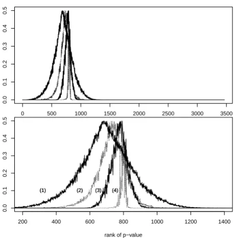
[image:5.595.183.412.65.298.2](1) (2) (3) (4) (1) (2) (3) (4)
Figure 1: Plot of the probability of a random decision min(pri,1−pri) for each hypothesis ordered by the rank of their p-value (naive method with 1000 permutations (1) and 10000 permutations (3) per hypothesis,QuickMMCTest with total effort K= 1000m (2) andK = 10000m (4)). Top shows all hypotheses, bottom shows a zoomed-in region around the last significant hypothesis.
time, ∆ =K/nmax has to be large enough to ensure that in line 13 of Algorithm 1, new samples
are drawn even for hypotheses with very low weights – this is needed to ensure that especially in the first iterations of Algorithm 1, no hypothesis is excluded preliminarily from receiving new samples in line 13. The influence of K andnmax (and thus of ∆ =K/nmax) on the accuracy of
QuickMMCTest is exemplarily demonstrated in Section ??of the Supplementary Material.
For an example run on generated p-values, Section?? of the Supplementary Material visu-alises how the sample allocation computed by QuickMMCTestcompares to the p-values and the testing threshold.
3
An application of multiple testing to gene expression data
We consider a dataset of gene modifications (so-called H3K4me2-modifications) of Pekowska et al. (2010): This dataset defines certain regions on a genome and specifies the midpoints of gene modifications within each region.
We are interested in testing whether the gene modifications appear more often in the lower half of the gene regions using the test of Sandve et al. (2011). For this, Sandve et al. (2011) first norm the beginning and the end of each region to 0 and 1, respectively. The midpoints of
k∈N gene modifications then correspond to krandom points X1, . . . , Xk in the interval [0,1]. We test the null hypothesis H0 :E(T)≥0.5 against the alternative H1 :E(T) <0.5 using the
test statistic T = 1k∑ki=1Xi in connection with a permutation test. For each gene region and its set of midpoints, a permutation is generated by permuting the locations of the midpoints in [0,1] while preserving all inter-point distances. Sandve et al. (2011) first filter the dataset for regions with at least 10 midpoints and define each such region to be one hypothesis. This leads tom= 3465 hypotheses under consideration.
and then tested all hypotheses by applying the Benjamini and Hochberg (1995) procedure with threshold 0.1. This was repeated r= 2000 times.
When applying the Benjamini and Hochberg (1995) procedure with a fixed threshold of 0.1, the allocation strategy based on Beta posteriors in QuickMMCTest is not yet used in the first iteration; instead, an equal weight is placed on each hypothesis (line 3 of Algorithm 1). Only after the inital batch of ∆ samples is drawn, the Benjamini and Hochberg (1995) procedure can be applied in all subsequent iterations to resampled p-values from the Beta posteriors and the constant threshold of 0.1 (line 8) in order to compute new weights (line 10) and to allocate further samples (lines 13 and 14 of Algorithm 1).
As done in Section 2.2 we quantify the uncertainty in these r test results by computing empirical probabilities pri (1−pri) that hypothesis i is rejected (non-rejected) among the r
repetitions. We define min(pri,1−pri)∈[0,0.5] as the probability of a random decision.
We repeat this experiment withQuickMMCTeston the same dataset an equal number of times and compute probabilities of a random decision. To ensure a fair comparison, we allow at most the same total number of samples the naive method had used, thus K = 1000m for low effort and K = 10000m for high effort, wherem is the number of hypotheses.
Figure 1 displays the probabilities min(pri,1−pri) of a random decision for the entire range of genes (top) in the Pekowska et al. (2010) dataset as well as for a zoomed-in region around the last significant hypothesis (bottom) occuring within the ranks 600−800. These curves correspond to the following methods: the naive method with 1000 permutations (1) and 10000 permutations (3) per gene as well as theQuickMMCTestalgorithm with a total effortK= 1000m
(2) andK = 10000m(4). Hypotheses are ordered according to the rank of their p-value estimate computed with 107 permutations. Due to the finite computational effort and the very low p-values the ordering of the hypotheses exhibits a certain noise.
Figure 1 (bottom) shows thatQuickMMCTestyields test results at a low effort (K = 1000m) with a level of uncertainty which is comparable to the one of the naive method at a high effort (10000 permutations per hypothesis). Using K = 10000m samples, QuickMMCTest yields test results which are considerably more stable and contain less random decisions than the ones of the naive method over the entire range of hypotheses.
Notably, comparing the location of the last rejected hypothesis (and thus the location of the peaks) in Figure 1 shows that, using the same computational effort, QuickMMCTestis able to re-ject more hypotheses than the naive method. This is a desired feature for practical applications. For datasets with few significant hypotheses, the number of rejections increases when spending more samples (or when allocating samples more efficiently as in the case of QuickMMCTest) due to the fact that higher numbers of samples (in connection with a pseudo-count in the numerator and denominator) give a higher resolution and capture more low p-values below the threshold.
4
Simulation study
We evaluate QuickMMCTest on a simulated dataset in three ways. First, the performance of
QuickMMCTest is compared to the one of the naive method using a variety of commonly used
Table 1: Average numbers of switched classifications (average numbers of switched rejections in brackets) for the naive method compared toQuickMMCTest(Alg. 1) for common multiple testing procedures. Constant testing threshold 0.1.
low effort (s= 1000) high effort (s= 10000)
naive Alg. 1 naive Alg. 1
Bonferroni (1936) 87 (0) 43.8 (2.6) 87 (0) 3 (1.7) Simes (1986) 32 (9.6) 2 (0.9) 9 (3.8) 0.1 (0.1) Hochberg (1988) 87 (0) 43.4 (2.5) 87 (0) 3.2 (2) Benjamini and Hochberg (1995) 31.9 (9.5) 2 (1) 9.1 (3.8) 0.1 (0.1) Benjamini and Yekutieli (2001) 162 (0) 14.5 (3.3) 22 (5.5) 0.6 (0.6) Sidak (1967) 90 (0) 36.3 (2.9) 90 (0) 3.5 (1.6) Holm (1979) 88 (0) 39.5 (3.2) 88 (0) 3.4 (2.1)
4.1 The simulation setting
In order to be able to compute numbers of switched classifications we need to simulate ex-ceedances of the sampled test statistic over the observed test statistic. For this it suffices to fix a set of p-values and simulate exceedances for the tests by sampling independent Bernoulli random variables with success probability being equal to the p-value of each test.
In Sections 4.2 and 4.3 we use one fixed set ofm= 5000 p-values. These p-values are indepen-dent realisations from a mixture distribution with a proportion 0.9 coming from a Uniform[0,1] distribution and the remaining proportion 0.1 coming from a Beta(0.25,25) distribution. A large proportion of p-values coming from the null would also be expected in practice. This model was used in Sandve et al. (2011).
Comparing the test result returned by any algorithm to the result obtained by applying the multiple testing procedure to the fixed set ofmp-values allows to compute numbers of switched classifications (see Section 2.1) with respect to the fixed p-values.
In Section 4.4, in each repetition of the experiment, we drawm Bernoulli random variables with probability 0.1. These random variables serve as indicators for the falseness of the null hypothesis. We then draw the p-value for each false null hypothesis from a Beta(0.25,25) distribution, and all remaining p-values from a uniform distribution in [0,1]. Comparing the decisions on all hypotheses computed by any algorithm to the falseness indicators thus allows to compute averages of type I error and power. In our multiple testing setting, we compute the per-pair power, defined as the average probability of rejecting a false null hypothesis.
All results are based on 1000 repetitions. The error of the simulations is less than the least significant digit we report in the tables presented in this section.
4.2 Comparison to a naive method for various multiple testing procedures
We compareQuickMMCTestto the naive method (Section 1) for a variety of commonly used mul-tiple testing procedures using the constant thresholdα∗= 0.1. These procedures are the step-up procedures of Bonferroni (1936), Simes (1986), Hochberg (1988), Benjamini and Hochberg (1995) and Benjamini and Yekutieli (2001) as well as the step-down procedures of Sidak (1967) and Holm (1979).
The naive method draws a fixed number ofs samples per hypothesis, estimates each p∗i as ˆ
pi= (ei+ 1)/(s+ 1) (Davison and Hinkley, 1997) and returnsh(ˆp, α(ˆp)), whereei is the number of exceedances observed for H0i,i∈ {1, . . . , m}, among ssamples and ˆp= (ˆp1, . . . ,pˆm).
cases apply QuickMMCTestwith a matched effort.
As stated in Section 2.2, computing final decisions on all hypotheses withQuickMMCTestby using empirical rejection probabilities as opposed to point estimates leads to both less switched classifications as well as a higher power (Sections ?? and ?? of the Supplementary Material). Results in this section (presented in Table??) are therefore given for empirical rejection proba-bilities only. Nevertheless, analogous results to the ones in Table 1 obtained withQuickMMCTest
in connection with point estimates can be found in Section ??of the Supplementary Material. Table 1 presents simulation results. When applying the naive method to the procedures of Bonferroni (1936) and Hochberg (1988) as well as Benjamini and Yekutieli (2001), Sidak (1967) and Holm (1979), the following phenomenon can be observed. Using a pseudo-count causes all p-value estimates ˆpi to be bounded below by 1/(ki+ 1), where i∈ {1, . . . , m}. Due to the low threshold used by the Bonferroni (1936) correction, this lower bound is larger than the testing threshold itself, leading to all hypotheses being consistently non-rejected and thus to meaningless results (see Section??in the Supplementary Material for more details). The number of recorded switched classifications is hence equal to the number of undetected rejections. For the Benjamini and Yekutieli (2001) procedure, results are meaningful only at a high effort.
The naive method is able to compute meaningful results at a low effort for the two procedures of Simes (1986) and Benjamini and Hochberg (1995) only, even though results still contain around 30 switched classifications on average. Most importantly, the naive method erroneously rejects considerably more hypotheses than QuickMMCTest (in the cases where rejections can be observed), thus reporting more false findings which is undesired in practice.
In contrast to the naive method,QuickMMCTestdoes not rely on computing p-value estimates and therefore computes meaningful results for all procedures at both a low and a high effort. At a low effort, these are very accurate for the procedures of Simes (1986) and Benjamini and Hochberg (1995). For all other methods, our approach yields around 35 to 45 switched classifications.
Applying the naive method at a high effort withs= 10000 samples per hypothesis is still not sufficient to observe any rejections for the procedures of Bonferroni (1936), Hochberg (1988), Sidak (1967) or Holm (1979). For all other procedures, the naive method yields around 10 to 20 switched classifications.
At a high effort, QuickMMCTest yields considerably less switched classifications than the naive method for all multiple testing procedures under consideration and essentially no switched classifications for the two procedures of Simes (1986) and Benjamini and Hochberg (1995). Similarly to the comparison at a low effort, our algorithm erroneously rejects considerably less hypotheses than the naive method, a feature desired for practical use.
The results of Table 1 are confirmed by a second study using a variable testing threshold which depends on the unknown p-values. To be precise, we correct the testing threshold using
α(p∗) = α∗/πˆ0(p∗), where α∗ = 0.1 and ˆπ0(p) = min (1,2/m
∑m
i=1pi) is a robust estimate of the proportion π0 of true null hypotheses of Pounds and Cheng (2006). Section ?? in the
Supplementary Material shows that the results for this variable testing threshold are qualitatively similar to the ones in Table 1.
4.3 Comparison to a variety of common methods
We now compareQuickMMCTestto previously suggested algorithms to test multiple hypotheses based on Monte Carlo sampling. These algorithms are the naive method and the algorithms of Besag and Clifford (1991), Guo and Peddada (2008), Sandve et al. (2011), Jiang and Salzman (2012) as well as Gandy and Hahn (2014). All methods are run with standard parameters sug-gested by their authors (the precise parameters are also listed in Section??of the Supplementary Material).
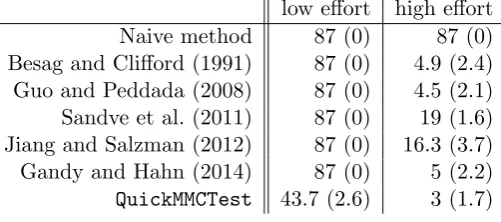
Table 2: Average numbers of switched classifications (average numbers of switched rejections in brackets) for common methods compared toQuickMMCTest using the Bonferroni (1936) correc-tion. Constant threshold 0.1.
low effort high effort
Naive method 87 (0) 87 (0)
Besag and Clifford (1991) 87 (0) 4.9 (2.4) Guo and Peddada (2008) 87 (0) 4.5 (2.1) Sandve et al. (2011) 87 (0) 19 (1.6) Jiang and Salzman (2012) 87 (0) 16.3 (3.7) Gandy and Hahn (2014) 87 (0) 5 (2.2)
[image:9.595.171.426.324.435.2]QuickMMCTest 43.7 (2.6) 3 (1.7)
Table 3: Average numbers of switched classifications (average numbers of switched rejections in brackets) for common methods compared to QuickMMCTestusing the Benjamini and Hochberg (1995) procedure. Constant threshold 0.1.
low effort high effort Naive method 31.9 (9.7) 9.1 (3.7) Besag and Clifford (1991) 18.3 (7.5) 18.3 (7.4) Guo and Peddada (2008) 4.5 (2.1) 0.3 (0.3) Sandve et al. (2011) 10 (4) 2.8 (1.3) Jiang and Salzman (2012) 13.2 (4.9) 3.5 (1.6) Gandy and Hahn (2014) 9.9 (4.1) 0.8 (0.6)
QuickMMCTest 2 (1) 0.1 (0.1)
where the naive method is used as a reference to set the total effort K. We define low effort as
K = 1000m, the effort equivalent to spending s= 1000 samples per hypothesis, and similarly high effort as K = 10000m. Results are displayed in Table 2.
For a low effort, Table 2 demonstrates that due to the very low threshold of the Bonferroni (1936) correction, all methods except forQuickMMCTestare unable to compute p-value estimates with a resolution sufficient to detect any rejections. They are thus unable to compute meaningful decisions, leading to switched classification numbers equal to the 87 rejections observed when applying the Bonferroni (1936) correction to the fixed p-values.
QuickMMCTest does not suffer from this problem and yields roughly 40 (out of m = 5000)
switched classifications with a very low number of false findings. If the computation of weights
in QuickMMCTestwas replaced by alternative approaches relying on discrete p-value estimates,
QuickMMCTest would be susceptible again to not being able to record any rejections like the
other methods considered in Table 2.
At a high effort, most methods compute acceptable test results with around 5 switched clas-sifications with the exception of the naive method which is still unable to detect any rejections.
QuickMMCTestyields a slightly lower average of switched classifications than the other methods.
50 100 200 500 1000 2000 5000 10000 20000
0.00
0.05
0.10
0.15
Number of samples
P
er−pair po
w
er
naive method QuickMMCTest
50 100 200 500 1000 2000 5000 10000 20000
0.0
0.1
0.2
0.3
0.4
0.5
0.6
0.7
Number of samples
P
er−pair po
w
er
[image:10.595.115.473.90.248.2]naive method QuickMMCTest
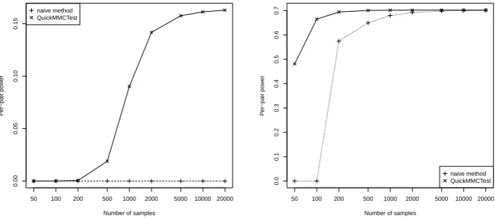
Figure 2: Average per-pair power against number of samples per hypothesis. Comparison of the naive method against QuickMMCTest for the Bonferroni (1936) correction (left) and the Simes (1986) procedure (right). Log-scale on the x-axis.
as Guo and Peddada (2008) and a multiple fold decrease compared to all other methods). At a high effort, Guo and Peddada (2008) perform comparably toQuickMMCTest.
These results are again consistent for a variable testing threshold as demonstrated in Section ??in the Supplementary Material (using the threshold of Pounds and Cheng (2006), see Section 4.2).
The similar performance of the algorithms of Guo and Peddada (2008), Gandy and Hahn (2014) as well as QuickMMCTest is not a coincidence. Both Guo and Peddada (2008) as well as Gandy and Hahn (2014) use a monotonicity property of step-up and step-down procedures of Tamhane and Liu (2008) to stop the sampling process for certain hypotheses in order to allocate the remaining samples equally to hypotheses whose decisions are computationally more demanding to compute. Neither of them uses any weights to fine-tune this equal allocation.
QuickMMCTest is able to both concentrate available samples on hypotheses whose decisions
are harder to compute as well as to fine-tune this allocation to individual hypotheses using weights, a feature which yields another improvement in accuracy compared to the other two methods.
4.4 QuickMMCTest yields a higher power
We compare the power of QuickMMCTestto the one of the naive method and selected algorithms used in Section 4.3 as a function of the number of samples per hypothesis. For this we use the simulation setting described in Section 4.1. As in Section 4.2, QuickMMCTest is applied with a matched total effort.
Figure 2 shows the average (per-pair) power of both the naive method andQuickMMCTestas a function of the number of samples. As seen previously in Table 2, due to the very low threshold of the Bonferroni (1936) correction, the naive method is not able to detect any rejections even for large numbers of samples (left plot in Figure 2). Its power is therefore zero. QuickMMCTest
initally suffers from the same problem, but is able to gain power when using an effort equivalent to 500 samples per hypothesis onwards. For the less conservative Simes (1986) procedure (right plot in Figure 2), the naive method gains power from 200 samples per hypothesis onwards.
QuickMMCTest achieves the same power as the naive method a lot faster with less samples: for
instance, the power of QuickMMCTestwith 100 samples per hypothesis is comparable to the one of the naive method with 1000 samples.
50 100 200 500 1000 2000 5000 10000 20000
0.00
0.05
0.10
0.15
Number of samples per hypothesis
P
er−pair po
w
er
Guo and Pedadda (2008) Besag and Clifford (1991) QuickMMCTest
50 100 200 500 1000 2000 5000 10000 20000
0.90
0.92
0.94
0.96
0.98
1.00
Number of samples per hypothesis
1−A
v
er
age f
alse non−disco
v
er
y propor
tion
[image:11.595.116.472.89.248.2]Naive method Guo and Pedadda (2008) QuickMMCTest
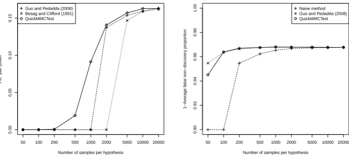
Figure 3: Left: Average per-pair power against number of samples per hypothesis. Com-parison of the algorithms of Guo and Peddada (2008) and Besag and Clifford (1991) against
QuickMMCTest. Multiple testing with the Bonferroni (1936) correction. Right: One minus the
average false non-discovery proportion against number of samples per hypothesis. Comparison of the naive method and the algorithm of Guo and Peddada (2008) against QuickMMCTest. Multiple testing with the Benjamini and Hochberg (1995) procedure. Log-scale on the x-axis.
QuickMMCTest to four selected existing methods already considered in Section 4.3.
Figure 3 (left) shows that for the Bonferroni (1936) correction,QuickMMCTestyields a much earlier incease in power for low samples sizes than the algorithms of Besag and Clifford (1991) and Guo and Peddada (2008), which in Table 2 both performed comparably well to QuickMMCTest. Figure 3 (right) repeats this comparison for the fdr analogue of the power, precisely 1−fnp, wherefnp is the false non-discovery rate, defined as the proportion of false negatives among the accepted null hypotheses. The plot shows that when controlling the false discoveries using the Benjamini and Hochberg (1995) procedure, both the algorithm of Guo and Peddada (2008) as well as QuickMMCTest achieve a higher power than the naive approach for low samples sizes, with a slight advantage for Guo and Peddada (2008).
In all comparisons presented in this section, the procedures kept the familywise error rate or the false discovery proportion at the α= 0.1 level, respectively.
The plots for power comparison of the naive method toQuickMMCTestusing the other multi-ple testing procedures considered in Section 4.2 are qualitatively similar to the ones in Figure 2. Similar to the left plot in Figure 3,QuickMMCTestalso outperforms all other methods considered in Section 4.3 in terms of the per-pair power when controlling the familywise error. With the exception of Guo and Peddada (2008), the same holds true when comparing QuickMMCTest to the methods considered in Section 4.3 in terms of 1−fnp similar to the right plot in Figure 3.
All comparisons in this article use QuickMMCTest with empirical rejection probabilities to determine decisions. Section ?? of the Supplementary Material repeats the power studies of Figures 2 and 3 when employing QuickMMCTest with both empirical rejection probabilities as well as point estimates to obtain decisions on all hypotheses after stopping. We show that empirical rejection probabilities lead to a higher power, especially for low computational effort.
5
Discussion
obtained if all p-values were known, as accurately as possible.
This article proposed to use an idea based on Thompson (1933) Sampling to efficiently allocate samples to multiple hypotheses. Our iterativeQuickMMCTestalgorithm is based on this principle and adaptively allocates more samples to hypotheses whose decisions are still unstable at the expense of allocating less samples to hypotheses whose decision can easily be computed. The algorithm works for a variety of common multiple testing procedures for both a constant as well as a variable testing threshold.
QuickMMCTesthas two main features: First, it never computes any p-value estimates during
its run, thus avoiding to incur consistently non-rejecting all hypotheses as observed in other methods published in the literature. Second, its final decisions are based on empirical rejection probabilities instead of p-value estimates.
QuickMMCTestwas evaluated in a simulation study. By comparing its performance to both a
widely used naive sampling method for a variety of commonly used multiple testing procedures as well as to a variety of algorithms published in the literature, we demonstrated thatQuickMMCTest
yields meaningful test results even at a low computational effort and up to a multiple fold decrease in the number of switched classifications at a high effort. For a low computational effort, QuickMMCTestyields a higher per-pair power across all methods considered in this study and, apart from the algorithm of Guo and Peddada (2008), a lower false non-discovery proportion when employed with various multiple testing procedures.
Supplementary Material
The Supplementary Material compares the performance of both QuickMMCTest variants using p-value estimates and empirical rejection probabilities. Moreover, it contains further simulation studies assessing the dependence of QuickMMCTeston its parameters: the total number of sam-ples K to be spent, the number of updatesnmax (and thus the number of samples ∆ =K/nmax
spent in each iteration) as well as the parameterR controlling the accuracy with which weights are computed. Moreover, the Supplementary Material repeats the simulation studies conducted in Section 4 for the variable testing threshold of Pounds and Cheng (2006).
Acknowledgements
We would like to thank the two referees for their constructive comments on the manuscript. The second author was supported by the EPSRC.
References
Agrawal, S. and Goyal, N. (2012). Analysis of Thompson Sampling for the Multi-armed Bandit Problem. JMLR: Workshop and Conference Proceedings of the 25th Annual Conference on Learning Theory, 23(39):1–26.
Asomaning, N. and Archer, K. (2012). High-throughput dna methylation datasets for evaluating false discovery rate methodologies. Comput Stat Data An, 56:1748–1756.
Benjamini, Y. and Hochberg, Y. (1995). Controlling the false discovery rate: A practical and powerful approach to multiple testing. J Roy Statist Soc Ser B, 57(1):289–300.
Benjamini, Y. and Yekutieli, D. (2001). The control of the false discovery rate in multiple testing under dependency. Ann Stat, 29(4):1165–1188.
Bonferroni, C. (1936). Teoria statistica delle classi e calcolo delle probabilit`a. Pubblicazioni del R Istituto Superiore di Scienze Economiche e Commerciali di Firenze, 8:3–62.
Davison, A. and Hinkley, D. (1997). Bootstrap Methods and Their Application. Cambridge University Press.
Dazard, J.-E. and Rao, S. (2012). Joint adaptive meanvariance regularization and variance stabilization of high dimensional data. Comput Stat Data An, 56:2317–2333.
Edgington, E. and Onghena, P. (1997). Randomization tests. Fourth Edition, Chapman & Hall/CRC, Boca Raton, FL.
Gandy, A. and Hahn, G. (2014). MMCTest – A Safe Algorithm for Implementing Multiple Monte Carlo Tests. Scand J Stat, 41(4):1083–1101.
Gleser, L. (1996). Comment on ’Bootstrap Confidence Intervals’ by T. J. DiCiccio and B. Efron. Statist. Sci., 11:219–221.
Guo, W. and Peddada, S. (2008). Adaptive choice of the number of bootstrap samples in large scale multiple testing. Stat Appl Genet Mol Biol., 7(1):1–16.
Gusenleitner, D., Howe, E., Bentink, S., Quackenbush, J., and Culhane, A. (2012). iBBiG: iterative binary bi-clustering of gene sets. Bioinformatics, 28(19):2484–2492.
Hochberg, Y. (1988). A sharper Bonferroni procedure for multiple tests of significance. Biometrika, 75(4):800–802.
Holm, S. (1979). A simple sequentially rejective multiple test procedure. Scand J Stat, 6(2):65– 70.
Jiang, H. and Salzman, J. (2012). Statistical properties of an early stopping rule for resampling-based multiple testing. Biometrika, 99(4):973–980.
Li, G., Best, N., Hansell, A., Ahmed, I., and Richardson, S. (2012). BaySTDetect: detect-ing unusual temporal patterns in small area data via bayesian model choice. Biostatistics, 13(4):695–710.
Liu, J. and Chen, R. (1998). Sequential monte carlo methods for dynamic systems. J Amer Statist Assoc, 93(443):1032–1044.
Liu, J., Huang, J., Ma, S., and Wang, K. (2013). Incorporating group correlations in genome-wide association studies using smoothed group Lasso. Biostatistics, 14(2):205–219.
Lourenco, V. and Pires, A. (2014). M-regression, false discovery rates and outlier detection with application to genetic association studies. Comput Stat Data An, 78:33–42.
Manly, B. (1997). Randomization, bootstrap and Monte Carlo methods in biology. Second Edition, Chapman & Hall, London.
Mart´ınez-Camblor, P. (2014). On correlated z-values distribution in hypothesis testing. Comput Stat Data An, 79:30–43.
Nusinow, D., Kiezun, A., O’Connell, D., Chick, J., Yue, Y., Maas, R., Gygi, S., and Sunyaev, S. (2012). Network-based inference from complex proteomic mixtures using SNIPE. Bioin-formatics, 28(23):3115–3122.
Pounds, S. and Cheng, C. (2006). Robust estimation of the false discovery rate. Bioinformatics, 22(16):1979–1987.
Rahmatallah, Y., Emmert-Streib, F., and Glazko, G. (2012). Gene set analysis for self-contained tests: complex null and specific alternative hypotheses. Bioinformatics, 28(23):3073–3080.
Rom, D. (1990). A sequentially rejective test procedure based on a modified Bonferroni inequal-ity. Biometrika, 77(3):663–665.
Sandve, G., Ferkingstad, E., and Nyg˚ard, S. (2011). Sequential Monte Carlo multiple testing. Bioinformatics, 27(23):3235–3241.
Shaffer, J. (1986). Modified sequentially rejective multiple test procedures. J Amer Statist Assoc, 81(395):826–831.
Sidak, Z. (1967). Rectangular confidence regions for the means of multivariate normal distribu-tions. J Amer Statist Assoc, 62(318):626–633.
Simes, R. (1986). An improved Bonferroni procedure for multiple tests of significance. Biometrika, 73(3):751–754.
Tamhane, A. and Liu, L. (2008). On weighted Hochberg procedures. Biometrika, 95(2):279–294.
Thompson, W. (1933). On the Likelihood that One Unknown Probability Exceeds Another in View of the Evidence of Two Samples. Biometrika, 25(3/4):285–294.
Wu, H., Wang, C., and Wu, Z. (2013). A new shrinkage estimator for dispersion improves differential expression detection in rna-seq data. Biostatistics, 14(2):232–243.