On the use of two time correlation functions for X ray photon correlation spectroscopy data analysis

warwick.ac.uk/lib-publications

Original citation:

Bikondoa, Oier. (2017) On the use of two-time correlation functions for X-ray photon

correlation spectroscopy data analysis. Journal of Applied Crystallography, 50 (2). pp.

357-368.

Permanent WRAP URL:

http://wrap.warwick.ac.uk/87391

Copyright and reuse:

The Warwick Research Archive Portal (WRAP) makes this work of researchers of the

University of Warwick available open access under the following conditions.

This article is made available under the Creative Commons Attribution 4.0 International

license (CC BY 4.0) and may be reused according to the conditions of the license. For more

details see:

http://creativecommons.org/licenses/by/4.0/

A note on versions:

The version presented in WRAP is the published version, or, version of record, and may be

cited as it appears here.

Received 30 September 2016 Accepted 11 January 2017

Edited by S. Boutet, SLAC National Accelerator Laboratory, Menlo Park, USA

Keywords: two-time correlation functions; X-ray photon correlation spectroscopy; data analysis.

On the use of two-time correlation functions for

X-ray photon correlation spectroscopy data analysis

Oier Bikondoa*

Department of Physics, University of Warwick, Gibbet Hill Road, Coventry CV4 7AL, UK, and XMaS, The UK–CRG Beamline, ESRF – The European Synchrotron, CS40220, F-38043 Grenoble Cedex 09, France. *Correspondence e-mail: [email protected]

Multi-time correlation functions are especially well suited to study non-equilibrium processes. In particular, two-time correlation functions are widely used in X-ray photon correlation experiments on systems out of equilibrium. One-time correlations are often extracted from two-time correlation functions at different sample ages. However, this way of analysing two-time correlation functions is not unique. Here, two methods to analyse two-time correlation functions are scrutinized, and three illustrative examples are used to discuss the implications for the evaluation of the correlation times and functional shape of the correlations.

1. Introduction

X-ray photon correlation spectroscopy (XPCS), the equiva-lent of dynamic light scattering using X-rays instead of visible light, is a powerful technique to study the dynamics of soft and hard condensed matter (Gru¨belet al., 2008; Sutton, 2008; Gutt & Sprung, 2015; Madsenet al., 2015; Bikondoa, 2016). XPCS allows one to probe the dynamics of fluctuations on short length scales (100 nm) and long time scales (104_{s) (Malik}

et al., 1998; Madsen et al., 2010). Information about the dynamics is obtained by studying the time correlation of the intensity scattered by a system in a dynamic regime when illuminated with coherent light. Under coherent illumination, the far-field pattern of light scattered by a sample shows a grainy intensity distribution called speckle (Sutton et al., 1991). The intermediate scattering function of the sample,

SðQ; Þ, is obtained from the normalized intensity auto-correlation of the speckles, gð2Þ_ð

Q; Þ, through the Siegert relation:1

gð2ÞðQ; Þ ¼

ItItþ

It

2

or

ItItþ

It

2

8 > > > > > > > > > < > > > > > > > > > :

9 > > > > > > > > > = > > > > > > > > > ;

¼1þðQÞ SðQ; Þ

Sð ÞQ

2

; ð1Þ

whereItandItþare the intensities at timestandtþand at

momentum transfer Q. is a delay time. The superscript (2) marks that the intensity autocorrelation is a second-order

ISSN 1600-5767

1

correlation on the electric field. The bar indicates an ensemble average over wavevectors with equivalent Q momentum transfer value and for which it is expected that the correlations are statistically equivalent. The bracketshidenote a time average.2SðQÞis the static structure factor. The optical contrastðQÞ ¼2_{=hIiis a factor that is used to account for}

the degree of spatial coherence of the incident radiation and is given by the variance of the intensity (2

) divided by its mean value (Madsen et al., 2010). The calculation of gð2Þ_ð

Q; Þ in equation (1) assumes that a time average can be performed over the entire measurement (Goodman, 1985). This assumption is valid for systems in equilibrium because for such systems the autocorrelation gð2Þ _{depends only on Qand the} time difference or delay timebetween measurements. That is, gð2Þ _{is time-shift invariant and does not depend on the} specific time when the measurement was made (observation time).gð2Þ_{ðQ; Þis a one-time correlation function (1-TCF).}

For non-equilibrium systems (i.e.for systems with average properties changing with time) the time average in equation (1) is not suitable because the dynamics are evolving and may strongly depend on the observation time. For those systems the evolution of the correlations can still be captured by using a more general expression than equation (1), namely a two-time correlation function (2-TCF) (Brownet al., 1997):

CorrðQ;t1;t2Þ ¼

It1It2 It1It2

I2

t1I

2

t1

1=2

I2

t2I

2

t2

1=2: ð2Þ

Corr is the autocovariance of the intensity normalized by its standard deviation. Different correlation functions are also used (Suttonet al., 2003):

GðQ;t1;t2Þ ¼

It1It2

It1It2

ð3Þ

or

CðQ;t1;t2Þ ¼DðQ;t1ÞDðQ;t2Þ; ð4Þ

where

DðQ;tÞ ¼ItIt

It

: ð5Þ

For random Gaussian fluctuations the standard deviation equals the average intensity (Brown et al., 1997; Loudon, 1983). Therefore, CðQ;t1;t2Þ ¼CorrðQ;t1;t2Þ 1 and the

different correlation functions [equations (2), (3) and (4)] are equivalent.

The use of 2-TCFs for XPCS was introduced, to our knowledge, by Brown et al. (1997), who studied the time correlations in the intensity scattered by a phase ordering system using numerical simulations. The 2-TCF is generally represented as a two-dimensional graph of the value of CorrðQ;t1;t2Þ, GðQ;t1;t2Þ or CðQ;t1;t2Þ for a fixed Q, with

axest1 andt2 (seex2.2). Brown et al. (1997) introduced an

alternative coordinate system, which has subsequently been widely used in the XPCS literature (Maliket al., 1998; Brown

et al., 1999; Livetet al., 2001; Suttonet al., 2003; Fluerasuet al., 2005; Ludwiget al., 2005; Fluerasuet al., 2007; Mu¨lleret al., 2011; Orsi et al., 2010, 2012; Chushkin et al., 2012; Livet & Sutton, 2012; Bikondoaet al., 2012; Rutaet al., 2012). Using this alternative coordinate system, approximated 1-TCFs are often extracted from the 2-TCF at different sample ages or observation times. We show below that in some cases employing such a coordinate system to extract approximate 1-TCFs may pose interpretation problems. For such cases, we put forward another coordinate system to extract the 1-TCFs and propose a clearer graphical representation of the 2-TCFs. This article is organized as follows: inx2 we describe the calculation of the autocorrelation (x2.1) and the two-time correlation function (x2.2) in discrete form. The extraction of 1-TCFs from the 2-TCF using different coordinate systems is examined inx3. Some properties of the 2-TCF for stationary and non-stationary systems, such as the time reversal symmetry, the functional shape and decay times, are analysed inx4. Model examples of 2-TCFs that reflect the differences between the analysis done using one coordinate system or another are presented inx5. A discussion about the coordinate system that should be used for different cases follows inx6. In

x7 we propose, in our view, a clearer graphical representation of the 2-TCFs. A summary (x8) and an appendix that intro-duces a geometric interpretation of the multi-time correlation functions in terms of metric spaces (Appendix A) close the article.

2. Calculation of the correlation functions

2.1. Autocorrelation function

We start by constructing the one-time correlation function (autocorrelation) for a generic set of data. The time auto-correlation function of a processuðtÞis defined by (Goodman, 1985)

ðQ; Þ:¼uðtþÞuðtÞ¼ lim T!1

1

T

ZT=2

T=2

uðtþÞuðtÞdt: ð6Þ

Let us consider that in a experiment we measure intensity fluctuations in time and at pointsQin reciprocal space.3 We 2

The order in which the time and ensemble averages are performed can be very important. For example, information about the ergodicity of the system may be lost if the time average is done before the ensemble average (Pusey & Van Megen, 1989), but when using area detectors the time average should be done first to preserve the speckle visibility and to be able to extract measurement errors directly from azimuthal variations ofgð2Þ_ð

Q; Þ(Lummaet al., 2000). However, multi-speckle dynamic light scattering (DLS)/PCS analysis is often done by performing the ensemble average first (Cipelletti & Weitz, 1999; Chushkinet al., 2012). Thus, the choice of the top or bottom formula between the braces in equation (1) depends on the case under study. This aspect is beyond the scope of this manuscript. For more details, see the aforementioned references.

3

can express a set of measured intensity fluctuations at different times as ann-tuple:

^

IIðQ;tÞ ¼ I0;I1;. . .;Ii1;Ii;Iiþ1;. . .;IN

; ð7Þ

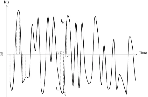
where the termsIjare the intensity fluctuations measured at timesj¼0;1;. . .;Nand are real numbers. A generic sample function is displayed in Fig. 1. The autocorrelation function is defined, in discrete form, by

gð2ÞðÞ ¼ 1 ðNþ1Þ

X

N

i¼0

Iiþi ; ð8Þ

where Iiþ

i ¼IiIiþ. The terms of equation (8) corresponding

to the different delay times () are shown in Table 1. There are

ðNþ1Þ terms for a given delay time. For ¼0, (N+ 1) terms are averaged, for¼1,Nterms and so on.

2.2. Two-time correlation function

If the process is not stationary, the statistical properties of the fluctuations will evolve over time. Thus, the summation and averaging that is done over the measurement time in equation (8) is not appropriate. A more general expression, namely a two-time correlation function (2-TCF), is obtained if the average in equation (8) is not performed. The 2-TCF is very useful to analyse the dynamics of non-equilibrium systems (Suttonet al., 2003). The temporal fluctuations and the variance of the 2-TCF are also used to investigate dynamical

heterogeneities in glassy systems through the analysis of higher-order correlations and multi-point dynamic suscept-ibilities [see Orsi et al. (2012) and Conrad et al. (2015) for recent XPCS work and references therein for details on the use of higher-order correlations to study dynamical hetero-geneities].

The 2-TCFCðQ;t1;t2Þis obtained by calculating the

Car-tesian product of II^ðtÞ [equation (7)] with itself (see also Appendix A for the calculation of the 2-TCF using the terminology of metric spaces) and ensemble averaging over equivalentQmomentum transfer vectors or pixels, when using a two-dimensional detector (Lummaet al., 2000):

CðQ;t1;t2Þ ¼II^II^¼

IN0 I N N

.. .

. .. ...

I0

i I

i

i I

N i

.. .

. .. ...

I0

0 I

N

0

0 B B B B B B @

1 C C C C C C A

: ð9Þ

The 2-TCF is a symmetric matrix by construction.4_{That is, the} 2-TCF is symmetric upon index swapping,i.e.8i;j:Iij¼I

i j, or, equivalently,Cðt1;t2Þ ¼Cðt2;t1Þ ¼Cðt1;t2Þ

T

, where T denotes the transpose operation. The time difference between two elements of the 2-TCF matrix is obtained using anL1_-metric

(also known as Manhattan, city-block or taxicab metric; Deza & Deza, 2014); the temporal distance (in units of scaled time) between two pointsIj1

i1 andI

j2

i2 is obtained from the sum of the

absolute value of the differences between their row and column indexes:

T¼ ji2i1j þ jj2j1j: ð10Þ

The elements with equal row and column indexes (terms of the formIi

i) are ‘equal-time’ terms. For a generic equal-time term

Ii

i, if the start of the experiment is taken ast¼0 fori¼0, the time elapsed from the start of the experiment istobs¼i. We

shall call this elapsed time the observation time tobs. The

temporal distancesT [equation (10)] can be converted into absolute time differences by multiplying them by the time step

t. The autocorrelation function equation (8) is obtained by averaging the terms along lines parallel to thet1¼t2diagonal.

3. Analysis of two-time correlation functions using different time coordinate systems

The evolution of the correlation functions is often quantified by selecting slices of the 2-TCFs at different observation times. These slices can be taken in different ways, using different coordinate systems. We discuss here the two most common procedures in the literature. Before proceeding, we should note, however, that other time variables such ast1,t2could also

be used to define an ‘observation time’.

Figure 1

Generic sample function of a random process II^ðtÞ fluctuating in time around its average valuehII^i. The time axis is divided into discrete time intervals.

Table 1

Terms at different delay timesthat are averaged when calculating the autocorrelation function [equation (8)].

Terms Number of terms

0 I0

0;I11. . .Iii. . .INN (N+ 1)

1 I1

0;I12. . .I

iþ1

i . . .INN1 ðNþ1Þ 1

2 I2

0;I13. . .I

iþ2

i . . .INN2 ðNþ1Þ 2

3 I2

0;I13. . .I

iþ3

i . . .INN3 ðNþ1Þ 3

I

0;I 1þ

1 . . .I

iþ

i . . .INN ðNþ1Þ

N IN

0 1

4

3.1. Conventional coordinate system

Starting from an equal-time term Ii

i in the 2-TCF matrix [equation (9)], 1-TCFs at different observation times can be extracted by taking the delay time along rows or columns in equation (9),i.e. lines witht1¼constant ort2¼constant. The

terms in these 1-TCFs have the formIiiþand the delay time is given by:¼ jt2t1j. This way of extracting 1-TCFs arises

directly from equation (8), removing the summation overiand the normalization factor that takes into account the number of terms summed for each delay time. We shall call this coordi-nate system the ‘conventional coordicoordi-nate system’ (CCS), although we note that this coordinate system is rarely used in the XPCS literature to analyse 2-TCFs. The terms at different delay times are shown in Table 2. The autocorrelation [equation (8)] is obtained from the 2-TCF by averaging the terms at equal delay timesof all the CCS-1-TCFs extracted at different observation times.

3.2. Alternative coordinate system

An ‘alternative coordinate system’ (ACS) was introduced by Brown et al.(1997) and has become the customary coor-dinate system in XPCS to analyse the 2-TCFs to extract 1-TCFs from them at different sample ages. In this ACS, the sample age is taken along thet1¼t2diagonal and defined as

tage:¼ ðt2þt1Þ=2. The delay time magnitude is the same as in

the CCS system (i.e. :¼ jt2t1j), but starting from an equal

termIi

i, the delay time direction is taken along lines perpen-dicular to thet1¼t2diagonal (see Fig. 2b). Cuts of the 2-TCF

along these perpendicular lines are 1-TCFs and are defined as ‘constant sample age’ cuts. These 1-TCFs are symmetric by construction around the ¼0 value. The terms at different delay times that are obtained for a given observation time

tobs¼i, following the definition of Brown et al. (1997), are

schematically shown in equation (11) (bold elements) and displayed in Table 2. Using the ACS, the autocorrelation function [equation (8)] is also obtained by averaging the terms at different delay times.

.. .

.. .

Ii2

iþ2 I

i1

iþ2 I

i

iþ2 I

iþ1

iþ2 I

iþ2

iþ2

Ii2

iþ1 I

i1

iþ1 I

i

iþ1 I

iþ1

iþ1 I

iþ2

iþ1

Ii2

i I

i1

i Iii ! Ii

þ1

i I

iþ2

i

# Iii12 I

i1

i1 I

i

i1 Ii

þ1 i1 ! I

iþ2 i1

# Ii2

i2 I

i1

i2 I

i

i2 I

iþ1

i2 Ii

þ2 i2 !

.. . .. . 0 B B B B B B B B B B B B B B B B B B B B B B @ 1 C C C C C C C C C C C C C C C C C C C C C C A

: ð11Þ

Table 2

Terms at different delay times extracted from the 2-TCF, following the conventions introduced inxx3.1 (CCS) and 3.2 (ACS).

For a delay timeto be accessible, the row and column numbers have to fulfil the inequalities specified above.

Terms

CCS ACS

0 Ii

i Iii

1 Iiþ1

i Ii

þ1

i

2 Iiþ2

i Ii

þ1

i1

3 Iiþ3

i Ii

þ2

i1

ðevenÞ Iiþ

i I

iþ=2N i=20

ðoddÞ Iiþ

i I

iþðþ1Þ=2N ið1Þ=20

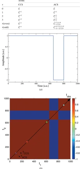
Figure 2

(a) Profile of the intensity. (b) Corresponding 2-TCF. The arrow running from the bottom left to the top right corner denotes the observation time. The delay time directions according to the CCS and ACS for an observation timetobs¼100 are indicated by the small arrows close to the

3.3. Differences between the CCS and ACS one-time correlation functions

There are essential differences between the 1-TCFs that are extracted using the conventional or the alternative coordinate systems. The CCS-1-TCF that passes through an equal-time term Ii

i has terms of the form I iþ

i , while the ACS-1-TCF comprises terms of the formIiiþ==220(even) orI

iþðþ1Þ=2

ið1Þ=20(

odd) (see Table 2). Thus, for a 1-TCF extracted for an obser-vation time5tobs¼Awe can note two differences:

(1) The terms of the CCS-1-TCF are of the formIAAþ and thus are directly related to the intensity measured at time

tobs¼A. On the other hand, in a ‘constant sample age’ cut of

the 2-TCF using the ACS, the terms have the formIAAþ: terms

obtained from the multiplication of intensities measured at times before and after tobs¼A are mixed (see terms in

Table 2). The ACS-1-TCF correlates terms that are equidistant (in time) from the observation timetobs¼A, but these terms

are not directly related to the intensity at the observation time

tobs¼A, except for the terms¼0.

(2) The number of terms of the 1-TCFs extracted for

tobs¼Ausing the CCS or the ACS are different. For the CCS,

the longest 1-TCF that can be extracted is attobs¼0

(begin-ning of the experiment). In contrast, using the ACS, the longest delay times accessible are for observation times

tobs’N=2, while the delay times accessible close to the start

or end of the experiment are much shorter (see Fig. 3). The first difference arises from the difficulty of defining precisely a ‘constant sample age’ in the case of time correla-tion funccorrela-tions. Time correlacorrela-tion funccorrela-tions are constructed by multiplying terms measured at different times. What happens at a certain time is related to another event at another time. ‘Constant sample age’ is then ambiguous and may be inter-preted or defined in different ways. On one hand, a ‘constant’ age may be considered what happens to the state of the sample at timetage¼Awhen it is related to its state at other times.

This interpretation would be in line with the analysis done using the CCS. Or it may be interpreted as what happens when events that occur before and after tage¼Aand at an

equidi-stant time delayare compared, which would correspond to the ACS analysis.

The second difference is just a consequence of the choice of the coordinate system. However, the direction in which the delay time is taken it is extremely important when performing quantitative analysis, because, for non-equilibrium systems, the relaxation times obtained from CCS- or ACS-1-TCFs will be different (seex5.3).

4. 2-TCFs for stationary and non-stationary systems

In stationary systems (strictly speaking, for wide-sense stationary systems; see Goodman, 1985), the 1-TCFs depend only on the time difference, not on the observation time. Therefore, the 2-TCF of a wide-sense stationary system is a

Toeplitz matrix, i.e. the following relationship between the terms of the 2-TCF holds:8i;j:Iji¼I

jþ1

iþ1. In addition, as the

2-TCF is symmetric around the t1¼t2 diagonal, then 8i;j:Iij¼Iji¼I

jþ1

iþ1¼I

iþ1

jþ1. The 2-TCF [equation (9)] of a

wide-sense stationary process thus has the form

CðÞ ¼

IN

0 I

i

0 I 0 0

.. .

. .. ...

Ii

0 I

0

0 I

i

0

.. .

. .. ...

I00 I

i

0 I

N

0

0 B B B B B B @

1 C C C C C C A

: ð12Þ

For wide-sense stationary systems, the CCS- and ACS-1-TCFs are therefore equivalent, except for the number of terms for each 1-TCF. The time symmetry is also maintained for stationary processes. The autocorrelation function of a real (i.e. not complex) stationary process has the following prop-erty (Goodman, 1985):

ðÞ ¼ðÞ: ð13Þ

This property is fulfilled for the CCS- and ACS-1-TCFs of stationary processes because 8i; :Iiiþ ¼I

i

i (CCS) and

Iiþ

i ¼I

i

iþ (ACS). However, in non-stationary processes

equation (13) does not necessarily hold (i.e.the time symmetry is broken). Besides, the 1-TCFs will generally depend on the observation timetobsand the delay time. The breakdown of

the time symmetry is well reflected in the CCS coordinate system: non-stationary processes yield asymmetric CCS-1-TCFs. However, even for non-stationary processes, equation (13) is fulfilled for the ACS-1-TCFs because they are symmetric by construction.

5. Examples

It is illustrative to compare the CCS-1-TCF and ACS-1-TCF for some model, extreme cases. Three examples are presented below: the first two examples are based on simple mathema-tical functions and the third is based on the integration of a partial differential equation that has been proposed to describe the evolution of a semiconductor surface upon ion beam sputtering (Castro et al., 2005). These examples have been chosen not for their physical relevance but because they reflect well some of the issues that arise when using different coordinate systems to extract 1-TCFs from 2-TCFs. The first example (x5.1: intensity following a step function) manifests that the ACS convention breaks the causality by mixing terms before and after an event has happened. In the second example (x5.2: sinusoidal intensity variation), the ACS-1-TCFs give skewed correlation functions and the skewness depends on the observation time. The third example (x5.3: 2-TCF of self-organized nanostructure formation dynamics on a surface due to sputtering) shows that, for an ageing system, the choice of the delay time direction has a direct effect on the correla-tion times and can also affect the funccorrela-tional shape of the correlation function.

In all the examples, we assume that the functions used in the calculations are representative of the dynamics of the system, 5

In the following, we consider that using the CCS the 1-TCF is extracted along the rows. If it were extracted along the columns, the result would be equivalent owing to the symmetry of the 2-TCF matrix along theIi

i.e. that proper corrections, normalization and ensemble averaging of the raw data have been performed, as would indeed be required in a real DLS or XPCS experiment (for details, seee.g.Chu, 2007; Wong & Wiltzius, 1993; Madsenet al., 2010; Madsenet al., 2015).

5.1. Correlation function of a step intensity function

We consider a dynamical system yielding intensity fluctua-tions in the scattered signal that can be described by a step function:

IðtÞ ¼

1 0tobsT1 1 T1<tobsT2

1 T2<tobsN

8 <

: ð14Þ

The signal profile is plotted in Fig. 2(a): the signal jumps from 1 to1 atT1¼650 and goes back to 1 atT2¼800. The

corresponding 2-TCF is shown in Fig. 2(b). CCS- and ACS-1-TCFs extracted at observation times t;;¼284;610;895

are displayed in Fig. 3.

We observe that the CCS-1-TCFs are correlated from the observation timetobs andt¼0 until the end of the period

(t¼T1;2tobs) and that in the following period they are

anticorrelated (i.e. C=1). However, the ACS-1-TCFs show correlation from the observation time until delay times that are twice those of the CCS-1-TCFs. This is due to the different delay time directions and the Manhattan geometry of the 2-TCF; the CCS-1-TCF follows a line while the ACS-1-TCFs follow a staircase trajectory [see equation (11)]. For this reason, the ACS-1-TCFs change sign at different delay times than the CCS-1-TCFs. The ACS-1-TCFs are correlated for delay times that are longer than the difference between the observation time and the switching of the intensity which, physically, is inconsistent.

5.2. Correlation function of a periodically oscillating intensity

Let us consider a system where, because of its dynamics, the scattered intensity fluctuates around a constant mean value in a sinusoidal way with angular frequency !. The intensity fluctuation can be represented asIðtÞ ¼cosð!tþ’₀Þ, where

’₀is the phase at timet¼0. For simplicity, we take’₀¼0 in the following. For such a signal, comparing the signal at timet

with itself for different delay times, it is expected that the correlation of the signal should vary periodically from positive to negative. The autocorrelation, as calculated using equation (6), is

CIðtÞIðtþÞðt; Þ ¼ IðtÞIðtþÞ

¼ ðcos!Þ=2: ð15Þ

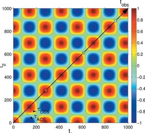
The 2-TCF is shown in Fig. 4. The terms of the 2-TCF have the formCi;j¼cos!icos!j. The 1-TCFs that are extracted from the 2-TCF following the CCS or the ACS convention have the following form:

CCS : CtobsðÞ ¼IðtobsÞIðtobsþÞ

¼cos!tobscos !ðtobsþÞ

;

ACS : CtobsðÞ ¼IðtobsþÞIðtobsÞ

¼cos!ðtobsþÞ

cos !ðtobsÞ

:

ð16Þ

The 1-TCFs extracted at tobs¼284, 610, 895 with !¼0:045

are shown in Fig. 5. Using the CCS, the (a priori) expected behaviour is reflected in the 1-TCFs, namely, the correlation oscillates periodically from positive values to negative ones andvice versa. The amplitude of the oscillations of a 1-TCF at

Figure 3

1-TCFs of the step function plotted in Fig. 2(a), extracted from its corresponding 2-TCF (Fig. 2b) at observation timestobs¼284, 610, 895,

using the CCS (solid blue line) or ACS (dashed red line).

Figure 4

2-TCF of a sinusoidally oscillating intensity (!¼0:045). The arrow running from the bottom left to the top right corner denotes the observation time. The delay time directions according to the CCS and ACS for an observation timetobs¼100 are indicated by the small arrows

timetobsis determined by the value ofItobsð¼0Þ ¼cos!tobs.

The amplitudes of the CCS-1-TCFs are symmetric around zero.

However, the 1-TCFs obtained with the ACS have a different behaviour: they may sometimes be always positive or negative. The behaviour of the 1-TCF extracted at tobs

following the ACS convention can be determined more easily by rewriting equation (16) as

ACS: CtobsðÞ ¼ðcos!tobscos!Þ

2

ðsin!tobssin!Þ 2

;

ð17Þ

where we have used trigonometric identities to rewrite the expression. The two terms in equation (17) are positive and

the amplitude of the ACS-1-TCFs will oscillate between

½sin2!t_obs;cos2_!t

obs. Thus, if sin!tobs¼0 (cos!tobs¼0),

CtobsðÞwill always be positive (negative). This can be observed

in the top panel of Fig. 5 (tobs¼284): the correlation is always

positive. For othertobs values, the amplitude variation of the

correlations is not symmetrical and will be skewed to positive or negative values unless sin!tobs¼cos!tobs.

5.3. Surface evolution under ion beam sputtering

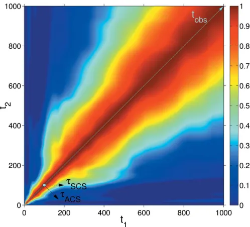
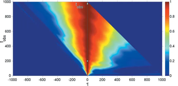
Ion beam sputtered surfaces are non-equilibrium systems that show ageing (Bikondoa et al., 2013). One theoretical approach to describe the temporal evolution and dynamics of such systems is the continuum theory, which uses partial differential equations to describe the evolution of the surface height (Mun˜oz-Garcı´aet al., 2009). Fig. 6 displays the 2-TCF obtained from numerical simulations integrating an equation that describes the evolution of semiconductor surfaces under ion bombardment [for more details on such systems and the calculation of the 2-TCF, see Bikondoa et al. (2012), and references therein]. In Fig. 7, we have extracted CCS and ACS 1-TCFs from Fig. 6, fortobs¼100. In the case of the

ACS-1-TCF (open circles), only delay values up to ¼200 are accessible. For the CCS-1-TCF (crosses), a delay time up to

¼900 can be extracted. The two 1-TCFs have been fitted using a stretched exponentialy¼exp½ðx=corrÞ

, wherecorr

is the correlation time and is the Kohlrausch–Williams– Watts exponent (Pecora, 2008). The value of the exponent

depends on the microscopic nature of the dynamics (Madsen

et al., 2010). Only the values in the ¼1!100 range have been used for the fit. This example shows (see values in Fig. 7) that, for a non-equilibrium system, there may be important differences in both the correlation times and theexponents that are obtained using one convention or the other. Such differences may be extremely important when interpreting

Figure 6

Contour plot of a 2-TCF for a model system that describes the evolution of a semiconductor surface under ion bombardment (Bikondoa et al., 2012). The directions of the delay time () for the CCS and ACS are indicated. The colour bar scale shows the degree of correlation. Figure 5

1-TCFs extracted from the 2-TCF of Fig. 4 at observation timestobs¼284,

610, 895, using the CCS (solid blue line) or ACS (dashed red line).

Figure 7

Example of one-time correlation functions attage¼100 extracted from

the 2-TCF of Fig. 6 using the convention of Brownet al.(1997) (open red circles) and the new convention proposed here (blue crosses). The dashed (black) and solid (green) lines have been obtained by fitting the one-time correlation data with the functiony¼exp½ðx=corrÞ

results from 2-TCFs and modelling the underlying dynamics (see theDiscussion).

6. Discussion

Which coordinate system should be used when analysing 2-TCFs and extracting 1-TCFs? A priori, either of the two coordinate systems can be used, provided, obviously, the comparison with theoretical models is done accordingly. This is the procedure followed in the pioneering work of Brownet al.(1997), in which computer simulations are used to study the statistical properties of speckles arising from the scattering of coherent radiation by a phase-ordering system. Theoretical models for such systems predict two-point, two-time correla-tion funccorrela-tions of the order parameter ðr;tÞ (i.e. the scalar field that describes the inhomogeneity of the system). The structure factor, which is obtained by averaging the scattered intensity over an ensemble of initial conditions, is related to the modulus square of the Fourier transform of the order parameter. Brownet al.(1997) analysed the intensity 2-TCFs using the ACS-1-TCF reference system, and the comparison with theoretical models and the scaling functions that they predict was done taking into account the ACS modified coordinates. The same procedure has been used in subsequent theoretical and experimental work on related or similar systems (Brownet al., 1997; Livetet al., 2001; Fluerasuet al., 2005). However, for most cases the interpretation of the CCS-1-TCFs is more straightforward because its calculation is in line with the usual way of calculating time correlation func-tions in statistical mechanics: a function of the state of the system at an initial time is multiplied by the value of the function at another, later timet; the autocorrelation function is defined as the ensemble average of that product (Zwanzig, 1965). CCS-1-TCFs are also in accordance with the use of dynamic correlations and response functions to analyse how a function of the system responds to a perturbation applied at a certain time tp [for an account of the relationships between

response and correlation functions, see Chaikin & Lubensky (1995) or Cugliandolo et al. (1994)]. The time symmetry is broken by applying an external field or force at timetp. The

response function will be nonzero only fort>tp. To account

for this, a step function dependence on the time is often included in the definition of the response function. As shown in the example ofx5.1, causality between terms of the corre-lation function is not retained for the ACS-1-TCFs and events that happen before and after the perturbation has occurred (i.e. tp) are then mixed. Thus, for the analysis of such systems,

the use of CCS-1-TCFs seems to be better suited. The same applies for quenched systems: ACS-1-TCFs would mix events prior and subsequent to the quenching. This could be avoided if the ACS analysis is restricted to areas in the TCF that are not crossed by any of the ‘events’. That would entail remaining inside a single square area (either red or blue, in Fig. 2) without crossing the boundary to another area.

Extracting CCS-1-TCFs from the 2-TCFs is an equivalent procedure to that employed to analyse the contact dynamics on granular piles subjected to weak vibrations using

multi-speckle diffusive wave spectroscopy (MDWS) (Kabla & Debre´geas, 2004). A waiting time is used to account for the number of vibrations the system has suffered before the measurement starts and a delay time for the number of vibrations after the waiting time. The waiting time is equiva-lent to the ‘observation time’ (tobs) that has been defined

above. The slow dynamics in glasses studied with dynamic light scattering have also been analysed in a similar manner, using a waiting time or sample age (Cipellettiet al., 2000). In these two studies, the 2-TCF is not explicitly employed. We note here that theories of non-equilibrium phenomena are generally expressed in terms of correlations that follow the CCS formulation (seee.g.Van Vliet, 2008; Berthieret al., 2011).

Ageing phenomena in glasses and other out-of-equilibrium systems have been extensively studied with XPCS using 2-TCFs and ACS-1-TCFs (Madsen et al., 2015; Bikondoa, 2016). Thus, to compare quantitative values extracted from ACS-1-TCFs with values obtained using other experimental techniques (e.g.MDWS or DLS) or theoretical predictions, it may be necessary to perform a coordinate change to analyse the results appropriately. Unfortunately, this point is not always clear in the literature. Instances can be found in which the width of the diagonal contour is taken as being propor-tional to the relaxation time (Rutaet al., 2013; Bikondoaet al., 2013) –i.e. the ACS-1-TCF convention is used – and where quantitative values of the relaxation time and the stretching parameter at different sample ages are reported. However, it would have been more natural to report quantitative values obtained following the CCS-1-TCF convention, as this is the one habitually used in glassy systems theory (Wolynes & Lubchenko, 2012). But because the ageing is so slow in the systems studied by Ruta et al. (2013) and Bikondoa et al.

(2013), the ACS- and CCS-1-TCFs are essentially equivalent. In other work (Mu¨lleret al., 2011), it is unclear if the 1-TCFs extracted from a 2-TCF that has sharp-cut division due to avalanche dynamics follow the CCS or the ACS convention. The example of the step function presented here in x5.1, suggests that the CCS-1-TCFs would be more suitable to analyse avalanche-type dynamics, and this may have been the procedure followed by Mu¨lleret al.(2011). But the reference provided by Mu¨lleret al.(2011) to explain how the 1-TCF has been calculated corresponds to work where the ACS-1-TCF was used (Maliket al., 1998). Which reference system has been used by Shinoharaet al.(2015) to extract 1-TCFs from 2-TCFs is not clear either. As there are different possible ways to extract 1-TCFs from 2-TCFs, it is important to explain precisely how the analysis has been carried out.

(1997) and in subsequent work on the non-equilibrium dynamics of ordering systems and first-order transitions (see the references in the Introduction). Notwithstanding, we remark that for equilibrium systems both coordinate systems lead to the same result and that for systems in quasi-equili-brium the quantitative differences may be minor. The 2-TCFs could certainly be analysed using other slicing methods if the dynamics under study and their physical interpretation require it. A generic procedure to extract one-time correlation func-tions from multi-time correlation funcfunc-tions is presented in AppendixA.

7. Alternative representation of the two-time correlation function

We propose an alternative way to display graphically the 2-TCF in a way that the CCS coordinate system is more apparent. The 2-TCF elements are plotted according to the following matrix:

I0

N INN

. . .

. .. ... .. .

I0

i I

i

i I

N i

. . .

.. .

. .. .. .

I0

0 I

N

0

0 B B B B B B @

1 C C C C C C A

: ð18Þ

For a generic matrix termIijin equation (18), the observation time is tobs¼i and the delay time ¼ij. Graphically

representing equation (18), the observation and delay times are along the vertical and horizontal axes, respectively (see Fig. 8). Negative/positive delay times correspond to going backward/forward in time. One advantage of this repre-sentation is that the 1-TCFs at different observation times are visualized more easily as horizontal lines. The autocorrelation function is obtained by averaging the rows instead of having to average diagonals. It also shows that with increasing sample age there are fewer terms for each of the 1-TCFs. In this graphical representation, the skewness and kurtosis of the peak at¼0 could be used to quantify the degree of

depar-ture from equilibrium and the correlation times. This assertion should still be cautioned: further theoretical developments are needed to verify if indeed the skewness and kurtoisis can meaningfully be related to the deviation from equilibrium, but the idea looks attractive.

8. Summary

We have compared two coordinate systems that are used to analyse two-time correlation functions and extract one-time correlation functions from them. We have shown that taking one-time correlation functions along rows or columns (CCS-1-TCFs) is more compatible with the way autocorrelation functions are generally calculated and theoretical results reported. In certain cases, these CCS-1-TCFs are more consistent physically and do not present causality problems. Importantly, the CCS-1-TCFs are not necessarily symmetric by construction and thus a lack of time symmetry indicates that the system is not stationary. For non-equilibrium systems, the correlation and delay times that are obtained with this coordinate system differ from the ones that are obtained using the convention introduced by Brown et al. (1997) (ACS-1-TCFs). A new graphical representation of the 2-TCFs has been introduced, where the observation time is represented along the vertical axis and the delay time along the horizontal.

APPENDIXA

Geometric description of multi-time correlation functions

We show here that multi-time (equivalently, multi-point) correlation functions can be conveniently expressed in terms of the formalism of metric spaces. Correlation functions of lower order are obtained using an adequate metric and defining a geometric trajectory in the multidimensional space. We describe how to construct generic -time correlation functions from operations between N-tuples and how one-time correlation functions can be extracted from them. We pay special attention to the¼2 case and the physical interpretation of the possible trajectories. We restrict ourselves to the correlation between only one variable. The generalization to correlations between different vari-ables (cross correlations) is straight-forward. A comprehensive discussion of arbitrary-order correlation functions using a tensor formalism, with special emphasis on coherence properties, is given by Mandel & Wolf (1995).

Let the tupleXðtÞ ¼ ðx0;x1;. . .;xNÞ be a set of measurements of the vari-able XðtÞ made at times t0;t1;. . .;tN. Thus, the tuple indexes 0;1;2;. . .;N

are related to the time the measure-ment was done. The time difference (or Figure 8

temporal distance) between measurements is t¼ jtjtij. Using the Cartesian product, we build an-dimensional array

Xð Þ ¼XX X¼Xi;j;...

¼ xi;xj;. . .

jxi;xj;. . .2X

; ð19Þ

where is the order of the correlation function we want to obtain. Each element of the array XðÞ is a tuple with

elements.

For each term in the array XðÞ¼Xi;j;..., we define the

function CðÞ ¼ fðXðÞÞ ¼ fðXi;j;...Þ ¼ xixj;. . ., where

i;j;. . .2 ½0;N. CðÞ is the product of the elements of each

-tuple and yields the correlation function of order. From

CðÞ, to extract anð1Þth-order correlation function we need to select aCð1Þ-dimensional subset ofCðÞ. Here, we sketch a method to obtain one-time correlation functions from an th-order correlation function.

First, we need to use a metric that defines the distance between the elements in theXðÞset. The set and the metric define a ‘metric space’ (Reed & Barry, 1980). To extract a one-time correlation function fromCðÞwe define a trajectoryT on

CðÞ,T CðÞ. Starting from a pointP2 CðÞ, the trajectory is chosen such that it joins points that are at consecutively larger distances in theCðÞgrid. The distance depends on the metric used.

The trajectories starting from a point P¼ ðp0;. . .;pÞ 2

XðÞ can be generically described as a set of points at succes-siverdistances fromP:

T ðP;rÞ ¼y2 X jdðy;PÞ ¼r ; ð20Þ

wheredðy;xÞis the metric. As explained above, for a generic elementXi;j;...¼ ðxi;xj;. . .Þ 2 X

ðÞ

, the indexes indicate which element of the tuple of measurements XðtÞ are being multi-plied when the function CðÞ¼fðXi;j;...Þ ¼xixj;. . . is calcu-lated, and are related to the time when the elements were measured. The Manhattan metric gives the distance between two elements in XðÞ as the sum of the absolute differences between their indexes:

dManðXi1;j1;...;Xi2;j2;...Þ:¼ kXi1;j1;...Xi2;j2;...k1

¼ i1i2

þ j1j2

þ ; ð21Þ

whereXi1;j1;... andXi2;j2;...are two generic points in X

ðÞ . The Manhattan distance corresponds to the casep¼1 of theLp norm (Deza & Deza, 2014):

x

k k:¼ P

i¼1

xi p 1=p

: ð22Þ

The Manhattan distance is the equivalent of the delay time. In an >1 grid, there are many different ways (‘trajectories’) to join points at monotonically increasing Manhattan distances. In general, the one-time correlation functions along different trajectories starting at a point P will not be equivalent. We analyse in the following the trajectories on¼2.

A1. Trajectories in a two-time correlation function

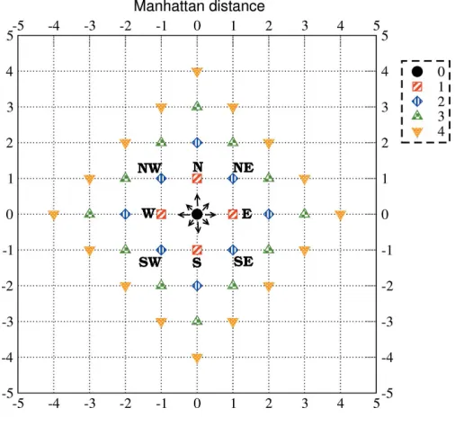
A 2-TCF can be represented by a two-dimensional grid or matrix (seex2.2). The Moore neighbourhood of a point in a two-dimensional grid is the set of points surrounding it (Deza & Deza, 2014). If we denote the surrounding points using four cardinal (N, E, S, W) and four intercardinal points (NE, SE, SW, NW), the equal-time diagonal (i.e.terms of the formXi;i) goes from the SW corner to the NE one (see Fig. 9). The allowed trajectories following one-unit step sizes of the Manhattan distance have individual steps going only along any of the four cardinal directions. With the Manhattan metric, trajectories along the intercardinal directions are obtained as staircase paths.Xð2Þ¼XXis symmetric by definition upon index swapping (i.e. Xi;j¼Xj;i), so we restrict ourselves to trajectories that remain in only one part of Xð2Þ_{, under the} equal-time diagonal. Under there requisites, the most relevant trajectories, or at least those with a clear physical interpreta-tion, are the trajectories starting at an equal-time point

P¼ ðp;pÞand which go only eastwards (E), southwards (S) or south-eastwards (SE):

E. The eastwards trajectory mixes the event (measurement) at point P with measurements done at later times. This trajectory is equivalent to the usual autocorrelation function [equation (8)] except that there is no average between the trajectories that start at every point of the equal-time diag-onal. The pair terms in the trajectory are of the form

ðp;pþÞ, whereis given by the Manhattan distance. Aver-aging all the E trajectories for every pointPon the equal-time diagonal, one obtains the usual autocorrelation function.

Figure 9

Manhattan distances on a two-dimensional grid. The Manhattan distances from point (0, 0) equal todMan¼0, 1, 2, 3, 4 are represented by a circle,

S. The southward trajectory relates the event (measure-ment) at point P with measurements done at earlier times. Thus, it can be interpreted as a correlation function where the delay time goes backwards in time. The terms in the trajectory are of the form ðp;pÞ. The S trajectory of any pointPis the same as the W trajectory. Averaging all the S trajectories for every pointPon the equal-time diagonal, one obtains the usual autocorrelation function.

SE. Using the Manhattan distance, the SE trajectory can only be obtained following a staircase-like trajectory. Depending on the choice of the term at a Manhattan distance equal to 1, the starting pointPwill be at the bottom or the top of the stair riser. In the SE trajectory, the event at timePonly appears in the term at Manhattan distances 0 and 1. Terms at

dMan2 relate events that happen before and after the event

atP. The terms are of the formðp;pþÞ.

E, S or purely SE trajectories can be obtained using a Chebyshev metric instead of the Manhattan one as the selecting rule for the terms along a trajectory. The Moore neighbourhood of a pointPis the set of points that are at a Chebyshev distance equal to 1. The Chebyshev metric corre-sponds to thep¼ 1case of theLpmetric [equation (22)] and is defined as follows:

dChðp;qÞ:¼ kpqk1¼max p1q1

; p2q2

: ð23Þ

Two points in a grid at distancedCh¼1 can be joined by a unit

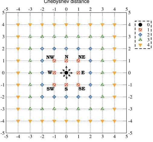
displacement along any of the cardinal or intercardinal directions,i.e.by the movement of the king on a chessboard (see Fig. 10). The Chebyshev distance is also called the ‘chessboard’ or ‘king-move’ metric (Deza & Deza, 2014). A

1-TCF extracted from an SE trajectory starting at a pointPof the equal-time diagonal and joining points at increasing Chebyshev distances is composed of terms arising from the multiplication of two events that happen at delay timesdCh

andþdCh, respectively (see Fig. 10).

There is an important difference between the 1-TCFs obtained using a Manhattan or a Chebyshev metric. The 1-TCFs obtained with a Manhattan metric always relate events that are at a unit delay time, whatever the direction of the steps is. However, using the Chebyshev metric, the delay time between the events that are related depends on the direction chosen. For 1-TCFs along only E or S (or staircase trajec-tories), the delay time is always 1. Along diagonals, the delay time between the related events is 2. That is, for a step with a Chebyshev distance equal to 1, the time step can in fact be 1 or 2.

It is clear that, depending on the metric used and the trajectories chosen, many different 1-TCFs can be constructed, which, in general, will not be equivalent. Other common metrics (for example, the Euclidean, which corre-sponds to the Lp with p¼2 case, and coincides with the Manhattan one if ¼1) can yield completely different 1-TCFs from the Manhattan or Chebyshev metrics. In this particular case of time-correlation functions, the Manhattan norm yields a clear physical picture for any dimensions, becausedMan ¼1 always relates events that are separated by

the same delay time, independently of the direction chosen in the-multidimensional space. For point (position) correlation functions obtained from measurements on a plane, Euclidean metrics would be better suited. The physics of the problem treated will determine which metric should be used.

Acknowledgements

OB gratefully acknowledges the financial support of the UK Engineering and Physical Sciences Research Council (EPSRC). The author would also like to thank Gerardina Carbone and Didier Wermeille for invaluable discussions.

References

Berthier, L., Biroli, G., Bouchaud, J.-P., Cipelletti, L. & Van Saarloos,

W. (2011). Dynamical Heterogeneities in Glasses, Colloids and

Granular Media.Oxford University Press.

Bikondoa, O. (2016).X-ray and Neutron Techniques for

Nanomater-ials Characterization, edited by C. S. S. R. Kumar. Berlin: Springer-Verlag.

Bikondoa, O., Carbone, D., Chamard, V. & Metzger, T. H. (2012).J.

Phys. Condens. Matter,24, 445006.

Bikondoa, O., Carbone, D., Chamard, V. & Metzger, T. H. (2013).Sci.

Rep.3, 1850.

Brown, G., Rikvold, P. A., Sutton, M. & Grant, M. (1997).Phys. Rev.

E,56, 6601–6612.

Brown, G., Rikvold, P. A., Sutton, M. & Grant, M. (1999).Phys. Rev.

E,60, 5151–5162.

Castro, M., Cuerno, R., Va´zquez, L. & Gago, R. (2005).Phys. Rev.

Lett.94, 016102.

Chaikin, P. M. & Lubensky, T. C. (1995).Principles of Condensed

Matter Physics.Cambridge University Press.

Figure 10

Chebyshev distances on a two-dimensional grid. The Chebybshev distances from point (0, 0) equal todCh¼0, 1, 2, 3, 4 are represented

Chu, B. (2007).Laser Light Scattering: Basic Principles and Practice.

Mineola: Dover Publications.

Chushkin, Y., Caronna, C. & Madsen, A. (2012).J. Appl. Cryst.45,

807–813.

Cipelletti, L., Manley, S., Ball, R. C. & Weitz, D. A. (2000).Phys. Rev.

Lett.84, 2275–2278.

Cipelletti, L. & Weitz, D. A. (1999). Rev. Sci. Instrum. 70, 3214–

3221.

Conrad, H., Lehmku¨hler, F., Fischer, B., Westermeier, F., Schroer, M. A., Chushkin, Y., Gutt, C., Sprung, M. & Gru¨bel, G. (2015).

Phys. Rev. E,91, 042309.

Cugliandolo, L. F., Kurchan, J. & Parisi, G. (1994).J. Phys. I,4, 1641–

1656.

Deza, M. & Deza, E. (2014). Encyclopedia of Distances, 3rd ed.

Heidelberg: Springer.

Fluerasu, A., Moussaı¨d, A., Madsen, A. & Schofield, A. (2007).Phys.

Rev. E,76, 010401.

Fluerasu, A., Sutton, M. & Dufresne, E. M. (2005).Phys. Rev. Lett.

94, 055501.

Forster, D. (1995). Hydrodynamic Fluctuations, Broken Symmetry

and Correlation Functions.Boulder: Westview Press.

Goodman, J. W. (1985).Statistical Optics.New York: John Willey and

Sons.

Gru¨bel, G., Madsen, A. & Robert, A. (2008). Soft Matter

Characterization, edited by R. Borsali & R. Pecora, pp. 953– 995. Berlin: Springer.

Gutt, C. & Sprung, M. (2015). X-ray Diffraction: Modern

Experi-mental Techniques, edited by O. H. Seeck & B. M. Murphy, pp. 385– 419. Singapore: Pan Stanford Publishing.

Kabla, A. & Debre´geas, G. (2004).Phys. Rev. Lett.92, 035501.

Livet, F., Bley, F., Caudron, R., Geissler, E., Abernathy, D., Detlefs,

C., Gru¨bel, G. & Sutton, M. (2001).Phys. Rev. E,63, 036108.

Livet, F. & Sutton, M. (2012).C. R. Phys.13, 227–236.

Loudon, R. (1983).The Quantum Theory of Light, 2nd ed. New York:

Oxford University Press.

Ludwig, K., Livet, F., Bley, F., Simon, J.-P., Caudron, R., Le Bolloc’h,

D. & Moussaid, A. (2005).Phys. Rev. B,72, 144201.

Lumma, D., Lurio, L. B., Mochrie, S. G. J. & Sutton, M. (2000).Rev.

Sci. Instrum.71, 3274–3289.

Madsen, A., Fluerasu, A. & Ruta, B. (2015).Synchrotron Radiation

and Free-Electron Lasers, edited by E. Jaeschke, S. Khan, J. R. Schneider & J. B. Hastings. Berlin: Springer.

Madsen, A., Leheny, R. L., Guo, H., Sprung, M. & Czakkel, O. (2010).

New J. Phys.12, 055001.

Malik, A., Sandy, A. R., Lurio, L. B., Stephenson, G. B., Mochrie, S. G. J.,

McNulty, I. & Sutton, M. (1998).Phys. Rev. Lett.81, 5832–5835.

Mandel, L. & Wolf, E. (1995). Optical Coherence and Quantum

Optics.Cambridge University Press.

Mo¨ller, J., Chushkin, Y., Prevost, S. & Narayanan, T. (2016). J.

Synchrotron Rad.23, 929–936.

Mu¨ller, L., Waldorf, M., Gutt, C., Gru¨bel, G., Madsen, A., Finlayson,

T. R. & Klemradt, U. (2011).Phys. Rev. Lett.107, 105701.

Mun˜oz-Garcı´a, J., Va´zquez, L., Cuerno, R., Sa´nchez-Garcı´a, J. A.,

Castro, M. & Gago, R. (2009).Toward Functional Nanomaterials,

edited by Z. M. Wang, pp. 323–398. New York: Springer.

Orsi, D., Cristofolini, L., Baldi, G. & Madsen, A. (2012).Phys. Rev.

Lett.108, 105701.

Orsi, D., Cristofolini, L., Fontana, M. P., Pontecorvo, E., Caronna, C.,

Fluerasu, A., Zontone, F. & Madsen, A. (2010).Phys. Rev. E,82,

031804.

Pecora, R. (2008).Soft Matter Characterization, edited by R. Borsali

& R. Pecora, pp. 953–995. Berlin: Springer.

Pusey, P. N. (2002).Neutrons X-rays and Light: Scattering Methods

Applied to Soft Condensed Matter, edited by P. Lindner & Th. Zemb, pp. 203–220. Amsterdam: Elsevier North Holland.

Pusey, P. N. & Van Megen, W. (1989).Phys. A Stat. Mech. Appl.157,

705–741.

Reed, M. & Barry, S. (1980). Methods of Modern Mathematical

Physics. I. Functional Analysis.New York: Academic Press.

Ruta, B., Baldi, G., Monaco, G. & Chushkin, Y. (2013).J. Chem. Phys.

138, 054508.

Ruta, B., Chushkin, Y., Monaco, G., Cipelletti, L., Pineda, E., Bruna,

P., Giordano, V. M. & Gonzalez-Silveira, M. (2012).Phys. Rev. Lett.

109, 165701.

Shinohara, Y., Yamamoto, N., Kishimoto, H. & Amemiya, Y. (2015).

J. Synchrotron Rad.22, 119–123.

Sutton, M. (2008).C. R. Phys.9, 657–667.

Sutton, M., Laaziri, K., Livet, F. & Bley, F. (2003).Opt. Express,11,

2268–2277.

Sutton, M., Mochrie, S. G. J., Greytak, T., Nagler, S. E., Berman, L. E.,

Held, G. A. & Stephenson, G. B. (1991).Nature,352, 608–610.

Van Vliet, C. M. (2008).Equilibrium and Non-equilibrium Statistical

Mechanics.Singapore: World Scientific.

Wolynes, P. G. & Lubchenko, V. (2012). Editors.Structural Glasses

and Supercooled Liquids: Theory, Experiment and Applications.

Hoboken: Wiley.

Wong, A. P. Y. & Wiltzius, P. (1993).Rev. Sci. Instrum.64, 2547–2549.