Rossiter McLaughlin models and their effect on estimates of stellar rotation, illustrated using six WASP systems

warwick.ac.uk/lib-publications

Original citation:

Brown, D. J. A., Triaud, A. H. M. J., Doyle, A. P., Gillon, M., Lendl, M., Anderson, D. R.,

Cameron, A. Collier, Hébrard, G., Hellier, C., Lovis, C., Maxted, P. F. L., Pepe, F., Pollacco,

Don, Queloz, Didier and Smalley, B.. (2016) Rossiter-McLaughlin models and their effect on

estimates of stellar rotation, illustrated using six WASP systems. Monthly Notices of the

Royal Astronomical Society.

http://dx.doi.org/10.1093/mnras/stw2316

Permanent WRAP URL:

http://wrap.warwick.ac.uk/82097

Copyright and reuse:

The Warwick Research Archive Portal (WRAP) makes this work by researchers of the

University of Warwick available open access under the following conditions. Copyright ©

and all moral rights to the version of the paper presented here belong to the individual

author(s) and/or other copyright owners. To the extent reasonable and practicable the

material made available in WRAP has been checked for eligibility before being made

available.

Copies of full items can be used for personal research or study, educational, or not-for profit

purposes without prior permission or charge. Provided that the authors, title and full

bibliographic details are credited, a hyperlink and/or URL is given for the original metadata

page and the content is not changed in any way.

Publisher’s statement:

This is a pre-copyedited, author-produced PDF of an article accepted for publication in.

Monthly Notices of the Royal Astronomical Society following peer review. The version of

Brown, D. J. A., Triaud, A. H. M. J., Doyle, A. P., Gillon, M., Lendl, M., Anderson, D. R.,

Cameron, A. Collier, Hébrard, G., Hellier, C., Lovis, C., Maxted, P. F. L., Pepe, F., Pollacco,

Don, Queloz, Didier and Smalley, B.. (2016) Rossiter-McLaughlin models and their effect on

estimates of stellar rotation, illustrated using six WASP systems. Monthly Notices of the

Royal Astronomical Society.

http://dx.doi.org/10.1093/mnras/stw2316

A note on versions:

The version presented here may differ from the published version or, version of record, if

you wish to cite this item you are advised to consult the publisher’s version. Please see the

‘permanent WRAP URL’ above for details on accessing the published version and note that

access may require a subscription.

Rossiter–McLaughlin models and their effect on estimates

of stellar rotation, illustrated using six WASP systems

?

D. J. A. Brown

†

, A. H. M. J. Triaud

, A. P. Doyle

, M. Gillon

, M. Lendl

,

D. R. Anderson

, A. Collier Cameron

, G. H´

ebrard

C. Hellier

, C. Lovis

,

P. F. L. Maxted

, F. Pepe

, D. Pollacco

, D. Queloz

, B. Smalley

1 _{Department of Physics, University of Warwick, Gibbet Hill Road, Coventry CV4 7AL, UK.}

2 _{Astrophysics Research Centre, School of Mathematics & Physics, Queen’s University, University Road, Belfast BT7 1NN, UK.} 3 _{Centre for Planetary Sciences, University of Toronto at Scarborough, 1265 Military Trail, Toronto, ON M1C 1A4, Canada} 4 _{Department of Astronomy & Astrophysics, University of Toronto, Toronto, ON M5S 3H4, Canada}

5 _{Institut d’Astrophysique et de G´eophysique, Universit´e de Li`ege, All´ee du 6 Aoˆut 17, 4000 Li´ege 1, Belgium} 6 _{Austrian Academy of Science, Space Research Institute, Schmiedlstraße 6, A-8042 Graz, Austria}

7 _{Observatoire Astronomique de l’Universit´e de Gen`eve, Chemin des Maillettes 51, CH-1290 Sauverny, Switzerland} 8 _{Astrophysics Group, Keele University, Staffordshire ST5 5BG, UK.}

9 _{SUPA, School of Physics and Astronomy, University of St Andrews, North Haugh, St Andrews, Fife KY16 9SS, UK.}

10_{Institut d’Astrophysique de Paris, UMR7095 CNRS, Universit´e Pierre & Marie Curie, 98bis boulevard Arago, F-75014 Paris, France} 11_{Observatoire de Haute Provence, CNRS/OAMP, F-04870 St Michel l’Observatoire, France.}

12_{Cavendish Laboratory, J J Thomson Avenue, Cambridge CB3 0HE, UK}

Accepted 0000 December 00. Received 0000 December 00; in original form 0000 October 00

ABSTRACT

We present new measurements of the projected spin–orbit angleλfor six WASP hot Jupiters, four of which are new to the literature (WASP-61, -62, -76, and -78), and two of which are new analyses of previously measured systems using new data (WASP-71, and -79). We use three different models based on two different techniques: radial ve-locity measurements of the Rossiter–McLaughlin effect, and Doppler tomography. Our comparison of the different models reveals that they produce projected stellar rota-tion velocities (vsinIs) measurements often in disagreement with each other and with estimates obtained from spectral line broadening. The Bou´e model for the Rossiter– McLaughlin effect consistently underestimates the value of vsinIs compared to the Hirano model. Although vsinIs differed, the effect on λ was small for our sample, with all three methods producing values in agreement with each other. Using Doppler tomography, we find that WASP-61 b (λ = 4◦.0+17₋₁₈._.1₄), WASP-71 b (λ =−1◦.9+7₋₇._.1₅), and WASP-78 b (λ=−6◦.4±5.9) are aligned. WASP-62 b (λ= 19◦.4+5₋₄._.1₉) is found to be slightly misaligned, while WASP-79 b (λ=−95◦.2+0₋₁._.9₀) is confirmed to be strongly misaligned and has a retrograde orbit. We explore a range of possibilities for the orbit of WASP-76 b, finding that the orbit is likely to be strongly misaligned in the positive

λdirection.

Key words: techniques: photometric – techniques: radial velocities – techniques: spectroscopic – planetary systems – stars: rotation

? _{based on observations (under proposal 090.C-0540) made using}

the HARPS high resolution ´echelle spectrograph mounted on the

ESO 3.6 m at the ESO La Silla observatory, and completed by

photometry obtained the Swiss 1.2mEulerTelescope, also at La

Silla.

† E-mail: [email protected]

1 INTRODUCTION

All eight planets of the Solar system orbit in approximately the same plane, the ecliptic, which is inclined to the solar equatorial plane by only 7.155±0◦.002 (Beck & Giles 2005). The orbital axes for the Solar system planets therefore ex-hibit near spin-orbit alignment with the Sun’s rotation axis (the origin of the slight divergence from true alignment is unknown). There is no guarantee, however, that this holds

true for extrasolar planets, as it is known that from binary stars that spin-orbit angles can take a wide variety of val-ues (e.g. Hube & Couch 1982; Hale 1994; Albrecht et al. 2007, 2009; Jensen & Akeson 2014; Albrecht et al. 2014). Compared to such systems, measurement of the alignment angle (‘obliquity’) for an extrasolar planet is more difficult owing to the greater radius and luminosity ratios. This is compounded by the face that the host star of a close-in exo-planet generally rotates more slowly than does the primary star in a stellar binary of the same orbital period. We are also generally limited to measuring the alignment angle as projected on to the plane of the sky, generally referred to as λ. Measurement of the true obliquity (ψ) requires knowledge of the inclination of the stellar rotation axis to the line of sight,Is, an angle that is currently very difficult to measure directly. It is possible to infer a value forIsusing knowledge of the projected stellar rotation speed, vsinIs, the stellar radius,Rs, and the stellar rotation period,Prot (e.g.Lund et al. 2014) , but the last of these can in turn be tricky to determine (e.g.Lendl et al. 2014).

HD 209458 b was the first extrasolar planet for which λwas measured (Queloz et al. 2000a). Since that work the number of systems for which the projected spin-orbit align-ment angle has been measured or inferred has been increas-ing at a steady rate, and is now closincreas-ing in on 100. By far the majority of these are transiting, hot Jupiter extrextrasolara-solar planets, and for most of these the value ofλhas been modelled using the Holt–Rossiter–McLaughlin (RM) effect (Holt 1983;Schlesinger 1910,1916;Rossiter 1924; McLaugh-lin 1924), the spectroscopic signature that is produced dur-ing a transit by the occultation of the red- and blue-shifted stellar hemispheres. Other, complementary methods such as Doppler tomography (DT, Collier Cameron et al. 2010a), consideration of the gravity darkening effect (e.g. Barnes, Linscott & Shporer 2011), modelling of photometric star-spot signatures (e.g. Nutzman, Fabrycky & Fortney 2011; Sanchis-Ojeda et al. 2011;Tregloan-Reed et al. 2015), mea-surement of the chromospheric RM effect in the Ca _II H & K lines (Czesla et al. 2012), and analysis of photomet-ric variability distributions (Mazeh et al. 2015) have also contributed to the tally.

While the vast majority of the measurements have been made via the RM effect, the models that have been used to model this effect have changed over time, becoming more complex and incorporating more detailed physics. The first models in widespread use were those of Ohta, Taruya & Suto(2005,2009) andGim´enez (2006), but these were su-perseded by the more detailed models ofHirano et al.(2011) and Bou´e et al. (2013), which take different approaches to the problem. A recent addition to the stable of RM mod-els is that of Baluev & Shaidulin (2015). This assortment of models means, combined with the variety of instruments with which RV measurements are made, might be introduc-ing biases into the parameters that we measure, particularly vsinIs andλ. These have yet to be fully explored.

In this work, we present analysis of the spin-orbit align-ment in six hot Jupiter systems, found by the WASP con-sortium (Pollacco et al. 2006), with the aim of shedding new light on the problems discussed above. We observed WASP-61 (Hellier et al. 2012); WASP-62 (Hellier et al. 2012); WASP-71 (Smith et al. 2013) WASP-76 (West et al. 2016);

WASP-78 (Smalley et al. 2012), and WASP-79 (Smalley et al. 2012).

These six systems were observed with HARPS under programme ID 090.C-0540 (PI Triaud). Our earlier RM ob-servation campaigns selected systems across a wide range of parameters and aimed to increase the number of spin-orbit measurements with as few preconceptions as possible. Here, we instead selected six particular objects. At the time, Schlaufman (2010), Winn et al. (2010) and Triaud (2011) had noticed intriguing relations between some stellar pa-rameters and the projected spin-orbit angle. Our selection of planets, orbiting stars withTeff around 6250 K, was meant to verify these.

2 METHODS

As in Brown et al. (2012a,b), we analyse the complete set of available data for each system: WASP photometry; follow-up photometric transit data from previous studies; follow-up spectroscopic data from previous studies; newly acquired photometric transit data, and newly acquired in-transit spectroscopic measurements of the RM effect using HARPS. New data are described in the appropriates sub-sections of Section3, and are available both in the appendix and online as supplementary information. Our modelling has been extensively described in previous papers from the Su-perWASP collaboration (Collier Cameron et al. 2007; Pol-lacco et al. 2008;Brown et al. 2012b, e.g.), but we summarize the process here for new readers.

Our analysis is carried out using a Markov Chain Monte Carlo (MCMC) algorithm using the Metropolis–Hastings de-cision maker (Metropolis et al. 1953; Hastings 1970). Our jump parameters are listed in Table1, and have been formu-lated to minimize correlations and maximize mutual orthog-onality between parameters. We use √esin(ω), √ecos(ω), √

vsinIsin(λ), and √vsinIcos(λ) to impose uniform pri-ors on e and vsinIs and avoid bias towards higher values (Ford 2006;Anderson et al. 2011). Several of our parameters (namely impact parameter,Teff, [Fe/H], and the Bou´e model parameters when appropriate) are controlled by Gaussian priors by default (see Table2). Others may be controlled by a prior if desired, see Section2.2.

At each MCMC step, we calculate models of the pho-tometric transit (followingMandel & Algol 2002), the Ke-plerian RV curve, and the RM effect (see following sec-tion). Photometric data is linearly decorrelated to remove systematic trends. Limb-darkening is accounted for by a four-component, non-linear model, with wavelength appro-priate coefficients derived at each MCMC step by interpo-lation through the tables of Claret (2000, 2004). The RV Keplerian curve, and thus the orbital elements, is primarily constrained by the existing spectroscopic data, as our new, in-transit spectroscopy covers only a small portion of the orbital phase. Quality of fit for these models is determined by calculatingχ2_.

s

We use a burn-in phase with a minimum of 500 steps, judging the chain to be converged (and thus burn-in com-plete) when χ2 _{for that step is greater than the median} χ2 of all previous values from the burn-in chain (Knutson et al. 2008). This is followed by a phase of 100 accepted steps, which are used to re-scale the error bars on the pri-mary jump parameters, and a production run of 104 ac-cepted steps. Five separate chains are run, and the results concatenated to produce the final chain of length 5×104 steps. The reported parameters are the median values from this final chain, with the 1σ uncertainties taken to be the values that enclose 68.3 percent of the distribution.

We test for convergence of our chains using the statistics of (Geweke 1992, to check inter-chain convergence) and ( Gel-man & Rubin 1992, to check intra-chain convergence). We also carry out additional visual checks using trace plots, au-tocorrelation plots, and probability distribution plots (both one- and two-dimensional). If an individual chain is found to be unconverged then we run a replacement chain, recal-culating the reported parameters and convergence statistics. This process is repeated as necessary until the convergence tests indicate a fully-converged final chain.

We have used the UTC time standard and Barycentric Julian Dates in our analysis. Our results are based on the equatorial solar and jovian radii, and masses, taken from Allen’s Astrophysical Quantities.

2.1 Modelling spin-orbit alignment

Our first model for the RM effect is that of Hirano et al. (2011). This has become the de facto standard thanks to its rigourous approach to the fitting procedure, which cross-correlates an in-transit spectrum with a template, and max-imizes the cross-correlation function (CCF). This method requires prior knowledge of several broadening coefficients, specifically the macroturbulence, vmac, and the Lorentzian (γH) and Gaussian (βH) spectral line dispersions. For this

work we assumed γH = 0.9 km s−1 in line with Hirano et

al., and also assumed that the coefficient of differential ro-tation,αrot= 01.βH is calculated individually for each RV

data set, and depends on the instrument used to collect the data as it is a function of the spectral resolution.

Bou´e et al. (2013) pointed out that the Hirano et al. model is poorly optimized for instruments which use a CCF based approach to their data reduction. For iodine cell spec-trographs (e.g. HIRES at the Keck telescope), theHirano et al.(2011) model works well, but for the HARPS data that we obtained for our sample theBou´e et al.(2013) model (as available via the AROME library2) should be more appropri-ate. The model defines line profiles for the CCFs produced by the integrated stellar surface out-of-transit, the uncov-ered stellar surface during transit, and the occulted stellar surface during transit, and assumes them to be even func-tions. The correction needed to account for the RM effect is calculated through partial differentiation, linearization, and maximization of the likelihood function defined by fitting a

1 _{Whilst several of the systems under consideration are rapidly}

rotating, without knowledge of the inclination of their stellar

ro-tation axes it is difficult to place a value onαrot.

2 _{http://www.astro.up.pt/resources/arome/}

Gaussian to the CCF of the uncovered stellar surface. This approach has been tested using simulated data, but has yet to be widely applied to real observations. In this paper, we will therefore compare its results to those from the two other models. To do so, we require values for the width of the Gaussian that is fit to theout-of-transit, integrated surface CCF (σ0), and for the width of the spectral lines expected if the star were not rotating (β0). The latter we set equal to the instrumental profile appropriate to each datum, whilst we use the former as an additional jump parameter for our MCMC algorithm, using the average results given by the HARPS quick reduction pipeline as our initial estimate and applying a prior using that value.

The DT approach was developed by Collier Cameron et al.(2010a) for analysis of hot, rapidly rotating host stars that the RM technique is unable to deal with. It has since been applied to exoplanet hosts with a range of parameters (Collier Cameron et al. 2010b; Brown et al. 2012b; Gan-dolfi et al. 2012;Bourrier et al. 2015). The alignment of the system is analysed through a comparison of the in-transit instrumental line profile with a model of the average out-of-transit stellar line profile. This latter model is created by the convolution of a limb-darkened stellar rotation pro-file, a Gaussian representing the local intrinsic line propro-file, and a term corresponding to the effect on the line profile of the ‘shadow’ created as the planet transits its host star. This ‘bump’ in the profile is time-variable, and moves through the stellar line profile as the planet moves from transit ingress to transit egress. Its width tells us the width,σ, of the lo-cal line profile, and is a free parameter. Since this width is measured independently, we can disentangle the turbulent velocity distribution of the local profile from the rotational broadening, measuring bothvsinIs andvmac directly. This gives DT an advantage over spectral analysis, as although it is possible to determine the turbulent velocity using the lat-ter method it requires spectra with very high signal-to-noise ratio (SNR). For work such as ours it is usually necessary, therefore, to assume a value forvmac.

The path of the bump is dictated bybandλ, and as the planet moves from transit ingress to transit egress its shadow covers regions of the stellar surface with different velocities. This leads to a relation betweenb,λ, andvsinIs, which must fit the observed stellar line profile when the local profile and rotational profile are convolved. We thus have two equations for two unknowns (vsinIsandσ, as bothbandλcan be de-termined from the bump’s trajectory), which are therefore well determined. Sinceλand vsinIs are independently de-termined using this method, it has the advantage of being able to break degeneracies that can arise between these two parameters in low impact parameter systems (Brown et al. 2012b, e.g.). We note, however, that this breaks down in systems with very slow rotation, i.e. where the uncertainty onvsinIsis comparable to the rotation velocity.

Another advantage that is often observed with DT is the improved precision on measurements of λthat it pro-vides, as seen byBourrier et al. (2015) for the case of the rapidly rotating KOI-12 system. This method also has po-tential as a confirmation method for planetary candidates, as seen with the case of recent case of HATS-14 b (Hartman et al. 2015), or conversely as a false positive identifier for difficult to confirm systems.

measure-Table 1.Details of the jump parameters that we use for our MCMC analysis. These parameters have been selected to maximize mutual

orthogonality, and minimize correlations. For detail of the priors, see Table2. Some composite jump parameters are indirectly controlled

by priors:esinwandecosware controlled by the prior on orbital eccentricity,e, whilevsinlandvcoslare controlled by the prior on

vsinIs.

Parameter Units Symbol Prior?

Epoch BJDTDB−2450000 t0 No

Orbital period days Porb No

Transit width days W No

Transit depth – d No

Impact parameter Stellar radii b Yes

Effective temperature K Teff Yes

‘Metallicity’ dex [Fe/H] Yes

RV semi-amplitude km s−1 _{K No}

√

esin(ω) – esinw indirectly; Yes/No

√

ecos(ω) – ecosw indirectly; Yes/No

Long-term RV trend – γ˙ Yes/No

√

vsinIsin(λ) (km s−1₎−1/2 _{vsinl indirectly; Yes/No}

√

vsinIcos(λ) (km s−1₎−1/2 _{vcosl indirectly; Yes/No}

Barycentric RV for CCFs km s−1 γRM Yes/No

FWHM for CCFs km s−1 FWHMRM No

Barycentric RV for RM data km s−1 γboue Yes

Bou´e model Gaussian width km s−1 _σ

boue Yes

Table 2.Details of the Bayesian priors that we apply during our MCMC analysis, and the values that were applied during thefinal

analysis of each system. Priors marked†are only applied during tomographic analyses, and are taken from the headers of the relevant

CCF FITS files. Priors marked‡are only applied during analyses using the Bou´e model for the RM effect, and are estimated from the

CCF FWHM in the FITS file headers.

System Parameter

Teff [Fe/H] b γRM† σboue‡

WASP-61 6250±150 −0.10±0.11 0.09±0.08 18.970±0.002 15.1±0.5

WASP-62 6230±80 0.04±0.06 0.29±0.11 14.970±0.005 12.8±0.5

WASP-71 6050±100 0.14±0.08 0.39±0.14 7.799±0.003 13.7±0.5

WASP-76 6250±100 0.19±0.10 0.14±0.10 −1.102±0.001 8.5±0.5

WASP-78 6100±150 −0.35±0.14 0.42±0.11 0.456±0.002 10.9±0.5

WASP-79 6600±100 0.03±0.10 0.71±0.03 4.9875±0.0004 25.0±0.5

ments by instrument, and further treat spectroscopic data taken on nights featuring planetary transits as separate data sets. Our Keplerian RV model considers these separated sets of data to be independent. To account for stellar RV noise, an additional 1 m s−1 is added in quadrature to the out-of-transit data; this is below the level of precision of the spectrographs used for this work.

2.2 Exploring system architectures

As in our previous work, we explore the possible solutions for each system using a combination of parameter constraints and initial conditions. We have four independent constraints that can be applied.

(i) Apply a Gaussian prior onvsinIs. This indirectly con-trols the jump parametersvsinlandvcosl.

(ii) Force the planet’s orbit to be circular, e = 0. This indirectly controls the jump parametersesinwandecosw. (iii) Force the barycentric system RV to be constant with

time, ˙γ= 0, neglecting long-term trends that are indicative of third bodies.

(iv) Force the stellar radius,Rs, to follow a main sequence relationship withMs,oruse the result from spectral analysis as a prior onRs.

We consider all 16 possible combinations of these four con-straints, analysing each case independently as described above. We discuss these analyses in the following sections. Once all combinations have been examined, we identify the most suitable combination by selecting that which provides the minimal value of the reduced chi-squared statistic,χ2

s

Figure 1. Upper panel: newly acquired EulerCam observations

of the transit of WASP-61 b, with the best-fitting model from MCMC analysis overlaid. No evidence of stellar activity is present. Lower panel: residuals of the data to the best-fitting model.

3 RESULTS

3.1 WASP-61

WASP-61 b orbits a solar metallicity, moderately rotating F7 star, and was initially identified using WASP-South. Follow-up observations using TRAPPIST (Jehin et al. 2011), Eu-lerCam (see Lendl et al. 2012for details of the instrument and data reduction procedure), and CORALIE (Queloz et al. 2000b) showed that the signal was planetary in origin (Hellier et al. 2012). The planet has a circular orbit with a period of 3.9 d, and has a relatively high density of 1.1ρJup. We observed the transit on the night of 2012 Decem-ber 22 using the HARPS high-precision ´echelle spectrograph (Mayor et al. 2003) mounted on the 3.6-m ESO telescope at La Silla. Fortuitously, we were able to simultaneously observe the same transit photometrically using EulerCam (white light; Fig.1). We use these new data in conjunction with all of the data presented in the discovery paper (in-cluding the original SuperWASP observations) to model the system using our chosen methods.

3.1.1 Hirano model

Trial runs with different combinations of input constraints revealed that the impact parameter of the system is low, ∼0.1. As expected, a degeneracy betweenvsinIsandλwas observed to be present, with the distinct crescent shaped posterior probability distribution covering a wide range of angles and extending out to unphysical values of vsinIs. OurvsinIs= 10.29±0.36 km s−1prior restricted the values of the two parameters as expected, but we felt that it was better to allow both to vary normally given our aim of

com-paring the various RM models. Tests with circular and ec-centric orbital solutions showed no evidence for an ecec-centric orbit, with the F-test ofLucy & Sweeney(1971) returning a less than 5 percent significance for eccentricity. This is also expected, as our new near- and in-transit RV measurements do not help to constrain the orbital eccentricity. Relaxing the stellar radius constraint led to insignificant variations in stellar density (which is computed directly from the photo-metric light curve, and therefore is distinct from the mass and radius calculations), but for some combinations of in-put constraints the value of the stellar mass varied by≈1σ. Tests for long-term trends in the barycentric velocity of the system returned results with strongly varying values of both positive and negative ˙γ, so we set this parameter to zero for our final runs.

The selected solution therefore does not apply a prior on vsinIs, assumes a circular orbit, neglects the possibility of a long-term trend in RV, and neglects the stellar radius con-straint. The fit to our data returnsχ2

red= 1.2. This particu-lar combination of applied constraints returns an projected spin-orbit alignment angle ofλ= 1◦.3+18−17..83, an impact pa-rameter ofb= 0.11+0−0..0907, and a projected rotation velocity ofvsinIs= 11.8+1−1..54km s

−1

, which is in agreement with the spectroscopic value ofvsinIs = 10.29±0.36 km s−1 deter-mined from the HARPS spectra usingvmac = 5.04 km s−1, itself derived using the calibration ofDoyle et al.(2014). The RM fit produced by the best-fitting parameters is shown in Fig.2.

3.1.2 Bou´e model

Similarly to the Hirano model tests, we found no evidence for an eccentric orbit (as expected), no reason to apply a constraint on the stellar radius, and no long-term trend in γ. The interaction with the prior onvsinIs was more inter-esting; with no prior the same degeneracy betweenvsinIs andλwas observed, but while applying the prior restricted the range of rotational velocities explored as expected, it led to a bimodal distribution inλ. Examination of the pos-terior probability distribution for the no-prior case revealed that this was caused by the Bou´e model under-predicting vsinIscompared to the spectroscopic value and the Hirano model, such that the prior from spectral analysis restricted the MCMC algorithm to values within the ‘tails’ of the cres-cent distribution. Checking posterior distributions for other parameters reveals that the MCMC chain is well converged, and our statistical convergence tests confirm this.

This highlights another degeneracy in the RM mod-elling problem, in addition to that between vsinIs and λ, where orbital configurations with (iorb,λ) and (iorb−π,−λ) produce the same ingress and egress velocities and the same chord length (Ohta, Taruya & Suto 2005;Fabrycky & Winn 2009). By extension therefore these configurations are indis-tinguishable when considering the two-dimensional problem, and the degeneracy can only be broken by considering the true alignment angle, ψ. This is particularly pernicious in the case of orbits withiorb ≈90◦. LikeFabrycky & Winn, we limit the inclination to the range 0◦6iorb690◦, which leads to the distribution shown in Fig.3, with solutions close to±40◦.

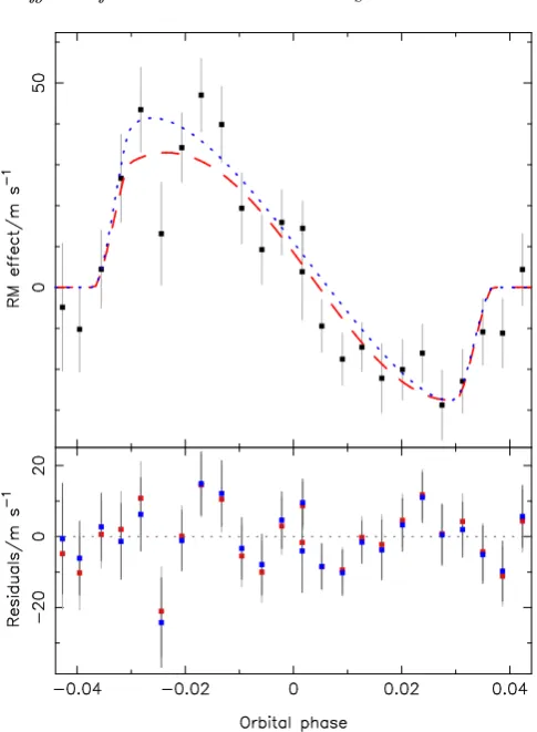
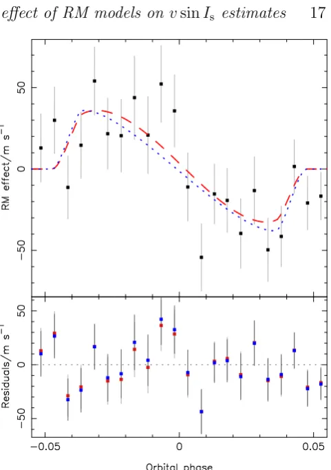
be-Figure 2.Upper panel: a close up of the RM anomaly in the RV curve of WASP-61, with the contribution from the Keplerian orbit subtracted to better display the form of the anomaly. The red, dashed line denotes the fit produced by the Hirano model, while

the blue, dotted line denotes the fit produced by the Bou´e model.

The two models clearly produce different fits to the spectroscopic data. Lower panel: the residuals for the two model fits. Red data with light grey error bars represent residuals for the Hirano model, while blue data with dark grey errors bars represent those for the

Bou´e model fit.

tween the two models, and acquire final results ofvsinIs= 8.9+3−1..27km s

−1

(consistent with, but lower than the Hirano value as expected from our tests), λ = 13◦.9+35.7

−39.6, and b = 0.09+0−0..1006. The resulting RM fit is shown in blue in Fig.2, which clearly indicates that the two models are fitting the same RM effect in different ways. The Bou´e fit exhibits steeper ingress and egress gradients, with sharper peaks at larger|velocity|than the Hirano model, which visually seems to provide a better fit to the RV data although neither model fits the second half of the anomaly particularly well. Com-paring their reducedχ2values though reveals that the Bou´e model gives a slightly poorer fit atχ2

red= 1.4, compared to the Hirano model’sχ2red= 1.2.

3.1.3 Doppler tomography

We applied the same set of constraints for our DT analysis as for the other two methods: no prior on vsinIs; ˙γ = 0; e = 0, and no constraint on the stellar radius. The stel-lar parameters returned were entirely consistent with those

0.00 0.05

−50 0 50 0

10 20 30

0.0 0.5

v sin i

*

/ km s

−1

λ / deg

. .

. .

Figure 3. The posterior probability distribution in iorb −

−λ parameter space for analysis of WASP-61 using the Bou´e

model while applying a prior on vsinIs using the value

de-rived from spectral analysis. The contours mark the 1σ, 2σ, and

3σconfidence regions. Also displayed are the marginalized,

one-dimensional distributions for the two parameters, with the

addi-tional, solid grey distribution invsinIsrepresenting the Bayesian

prior. This distribution highlights the degeneracy that arises

be-tween solutions with (iorb,λ) and (iorb−π,−λ)

from both the Hirano and Bou´e models. With results of vsinIs= 11.1±0.7 km s−1,λ= 4◦.0+17−18..14, andb= 0.10

+0.10

−0.06,

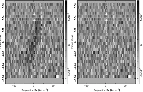
we find no discrepancy between DT analysis and the two other techniques for modelling the RM anomaly. The left-hand panel of Fig.4shows the time series of the CCFs, with the prograde signature of the planet barely visible. No sign of stellar activity is visible in the CCF residual map.

s

Figure 4. Time series map of the WASP-61 CCFs with the

model stellar spectrum subtracted. The signature of the planet is just about visible moving from the lower left corner to the up-per right corner, indicating a prograde orbit across both stellar hemispheres. The symmetry about the central line is indicative of

an aligned system. Time (phase) increases vertically along they

-axis, with the horizontal dotted line marking the mid-transit time (phase). The vertical dotted line denotes the barycentric

veloc-ityγ, whilst the vertical dashed lines indicate±vsinIfrom this,

effectively marking the position of the stellar limbs. The crosses mark the four contact points for the planetary transit. The back-ground has been set to grey to aid clarity.

3.2 WASP-62

Like WASP-61 b, WASP-62 b was discovered through a com-bination of WASP-South, EulerCam, and Trappist photom-etry, in conjunction with spectroscopy from CORALIE ( Hel-lier et al. 2012). The host star is again a solar metallicity, F7-type star, and the planet has a circular orbit of period 4.4 d. WASP-62 b is rather inflated (Rp= 1.39±0.06RJup) com-pared to its mass (Mp= 0.57±0.04MJup), leading to a much lower density of 0.21ρJup. Analysis of the HARPS spectra givesvsinIs = 8.38±0.35 km s−1, withvmac= 4.66 km s−1 from the calibration ofDoyle et al.(2014); it is these values that we use for our prior onvsinIs.

HARPS was used to observe the spectroscopic transit on the night of 2012 October 12. Additional RV measure-ments were made using the same instrumeasure-ments on 2012 Oc-tober 15–17 to help constrain the full RV curve. We use the full set of available data to characterize the system, includ-ing the weather-affected EulerCam light curve; asHellier et

0.00 0.02 0.04

−50 0 50 0

10 20 30

0.0 0.5

v sin i

*

/ km s

−1

λ / deg

. .

. .

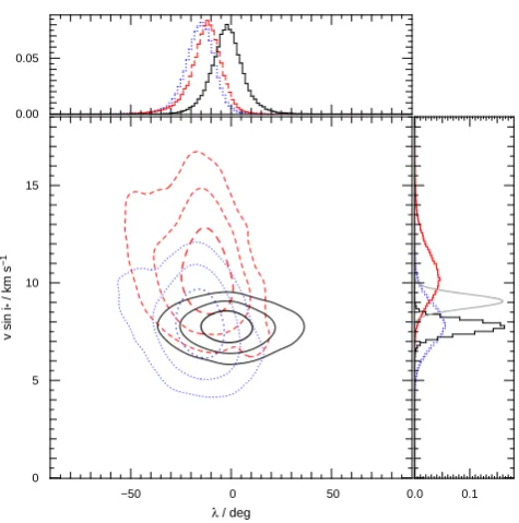
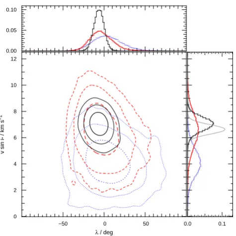
Figure 5. The posterior probability distribution in vsinI−λ

parameter space for the Hirano model (red, dashed contours),

Bou´e model (blue, dotted contours), and DT (black, solid

con-tours) analyses of WASP-61. The contours mark the 1σ, 2σ, and

3σconfidence regions. Also displayed are the marginalized,

one-dimensional distributions for the two parameters; the different models are distinguished as for the main panel, and the

addi-tional, solid grey distribution invsinIsrepresents the result from

spectral analysis. Theλ1D distribution shows that although

to-mography improves the precision in the alignment by a factor of 2, it provides no improvement over the Hirano model. The

im-provement for this system comes invsinIs, where the uncertainty

reduces by approximately 50 percent when tomography is used.

Note the crescent shape of the Bou´e distribution, even at the 1σ

level, whereas the distributions for the other models show less structure.

al.(2012) note, the MCMC implementation that underlies our analysis accounts for this poorer quality data.

3.2.1 RM modelling

Trial runs to test the effect of applying the four input con-straints found that there was no long-term trend in barycen-tric velocity, and no evidence for an eccenbarycen-tric orbit, with ei-ther of the two RM models. Relaxation of the stellar radius constraint led to only minor changes in the reported stel-lar parameters, with stelstel-lar mass and radius being entirely consistent whether the constraint was enforced or not.

Figure 6. Upper panel: a close up of the RM anomaly in the RV curve of WASP-62, with the contribution from the Keplerian orbit subtracted to better display the form of the anomaly. Lower panel: the residuals for the two model fits. Legends for the two

panels as for Fig.2.

produces larger 1σ uncertainties in the value ofλin order to compensate when trying to fit the RM effect. This effect can be seen in Fig.8, with the 1σcontours for these models being completely distinct. For both models, the alignment angle value remained pleasingly consistent across the differ-ent constraint combinations.

The full sets of results, which were produced from runs using no prior on vsinIs, no constraint on Rs,e = 0, and

˙

γ = 0, can be found in Table5, and show that the larger impact parameter has enabled more stringent limits to be placed on the spin-orbit alignment angle than was the case for WASP-61. Fig.6 shows that the two models again pro-duce dissimilarly shaped best-fitting RM models; as with WASP-61, the Bou´e model has steeper ingress and egress velocity gradients, and sharper peaks. However, the angles produced by the two models are entirely consistent, with the Hirano model finding λ = 19◦.1+6−5..48 and the Bou´e model λ= 18◦.9+11−6.6.5.

3.2.2 Doppler tomography

Using the same set of input constraints as for our RM mod-elling, we again carried out DT analysis of the system, find-ing an alignment angle ofλ= 19◦.4+5−4..19. The planetary sig-nature of 62 is much stronger than that of

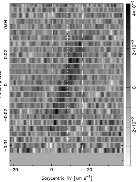
WASP-Figure 7. Time series map of the WASP-62 CCFs, following

subtraction of a model stellar spectrum. The planetary signa-ture, moving from lower left to upper right, is unambiguous. A prograde, symmetrical orbit is clearly implied, in agreement with

the form of the RM effect. Legend as Fig.4.

61, and can be seen far more clearly in the CCF time series map (Fig.7). For this system, the tomographic method has improved the uncertainties on λ by roughly a factor of 2 compared to the Bou´e model, but again provides little im-provement over the precision afforded by the Hirano model. All three results are consistent with alignment according to the criterion ofTriaud et al. (2010), a conclusion which is supported by the trajectory of the planetary signal in Fig.7. However, this is based on an ad hoc criterion that reflects the typical uncertainty onλmeasurements at the time that it was formulated. Work since 2010 has improved the typical uncertainty, such that this criterion is no longer really appli-cable. We therefore classify WASP-62 as slightly misaligned; the resolution of the planet trajectory in our Doppler map is insufficient to distinguish this from a truly aligned orbit.

s

0.00 0.05

0 20 40 60 0

5 10 15

0.0 0.2

v sin i

*

/ km s

−1

λ / deg

. .

. .

Figure 8.The posterior probability distributions invsinI−λ

pa-rameter space for our analyses of WASP-62. Legend as for Fig.5.

The three models give distinct 1σ solutions in vsinIs for this

system, but provide similar precision in λ. Note that the Bou´e

distribution shows an extended tail inλcompared to the other

models.

3.3 WASP-71

Smith et al. (2013) presented the discovery of WASP-71 b using photometry from WASP-N, WASP-South and TRAPPIST, along with spectroscopy from CORALIE that included observations during transit made simultaneously with the TRAPPIST observations. The host star was found to be an evolved F8-type, and significantly larger and more massive than the Sun, whilst the planet was found to be in-flated compared to the predictions ofBodenheimer, Laugh-lin & Lin (2003, e.g.), and to have a circular orbit with a period of 2.9 d. The spectroscopic transit observations made using CORALIE enabledSmith et al. to measure the pro-jected spin-orbit alignment angle of the system. They found that the system was aligned, with λ = 20◦.1±9.7, and rapidly rotating atvsinIs= 9.4±0.5 km s−1 (calculated as-sumingvmac= 3.3±0.3 km s−1followingDoyle et al. 2014). We obtained additional spectroscopic data on the night of 2012 October 26, observing a complete transit, with fur-ther observations made on 2012 October 23 and 25. We com-bine these with the discovery photometry and spectroscopy to model the system. We do not, however, include the spec-troscopic transit used bySmith et al.to measureλ, for two reasons. The first is that we wish to obtain an independent measurement of the spin-orbit alignment. The second is that, as noted byBou´e et al.(2013), different instruments can pro-duce different signals from the same measurement owing to their different analysis routines, and therefore RM data sets from different instruments should not be combined. Analysis of our new HARPS spectra givesvsinI= 9.06±0.36 km s−1 andvmac= 4.28 km s−1.

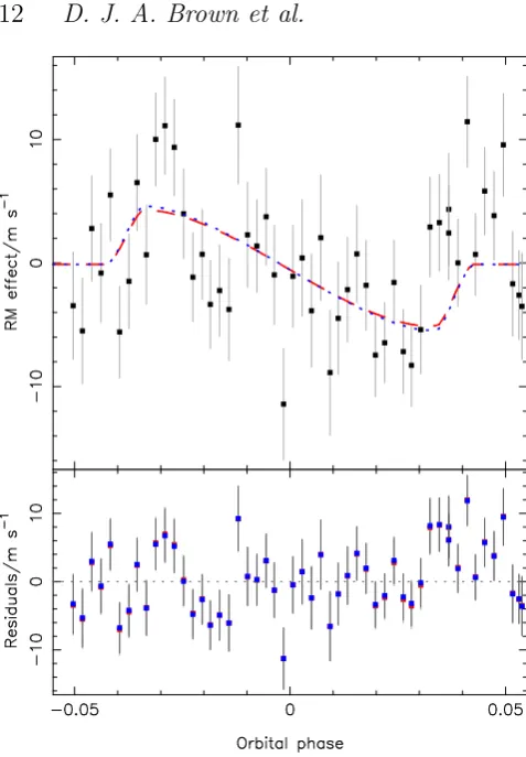
Figure 9.Upper panel: a close up of the RM anomaly in the

RV curve of WASP-71, with the contribution from the Keplerian orbit subtracted to better display the form of the anomaly. Lower panel: the residuals for the two model fits. Legends for the two

panels as for Fig.2.

3.3.1 RM modelling

Using the F-test ofLucy & Sweeney(1971) we found no indi-cation of significant eccentricity in the system, in agreement withSmith et al.(2013), and therefore sete= 0 in our final analysis. We also found no consistent evidence that there is a long-term trend in barycentric velocity, so set ˙γ= 0.

The interaction betweenvsinIs, b, and the stellar ra-dius constraint is an interesting one for this system. Relaxing the constraint onRscauses the stellar radius to decrease by

whilst neglecting the constraint gives a temperature more consistent with previous analyses.

Once again, we find that the two different methods re-turn similar results for the alignment angle and stellar pa-rameters, but that the Bou´e model gives a more slowly rotat-ing star than is suggested by the Hirano model (see Table5). Fig.9shows the best-fitting models produced by both meth-ods, with the Hirano model (the dashed, red line) having a shallower peak during the first half of the anomaly. There is substantial scatter in the RV measurements during this period however, and the Hirano model appears to better fit the second half of the anomaly, where there is less scatter in the radial velocities.

The final solutions that we report were taken from runs with no prior on vsinIs, e = 0, ˙γ = 0, and no constraint applied to the stellar radius.

3.3.2 Doppler tomography

Whereas for the two previous systems the tomographic anal-ysis supported the Hirano model with regards to the pro-jected rotation velocity of the host star, for WASP-71 it is the Bou´e model with which DT agrees (see Fig.10), al-though the value of 7.8±0.3 km s−1 _{that we find is} signif-icantly lower than the spectroscopic value. The other pa-rameter values that are found through DT are substantially different to either set of RM results. The impact parame-ter is lower, leading to a lower value ofλthat is consistent with 0◦(see Table5). Particularly interesting though is the difference in the physical stellar parameters found by this method, which imply a smaller star. As implied by our result ofλ=−1◦.9−+77..15, Fig.11shows that the system is well char-acterizedaligned, in agreement with the result fromSmith et al.(2013), although we are not able to significantly improve on the precision that they report.

3.4 WASP-76

WASP-76 A (West et al. 2016) is another F7-type planet-hosting star, but is rotating significantly more slowly than either WASP-61 or WASP-62. The planet is substantially bloated, with a density of only 0.151±0.010ρJup, and orbits its host every 1.8 days in a circular orbit. It was discovered and characterized using data from WASPSouth, TRAP-PIST, EulerCam, SOPHIE (Bouchy et al. 2009;Perruchot et al. 2011), and CORALIE.

HARPS was used to observe the transit taking place on 2012 November 11, and to make additional measurements on 2012 November 12–14. We combined these measurements with the discovery paper’s photometry for our analysis, ex-cluding two spectra that were obtained at twilight. Spectral analysis of the new spectra returned vmac = 4.84 km s−1 using the calibration of Doyle et al. (2014), leading to vsinIs = 2.33±0.36 km s−1. We use this for our prior on rotation velocity. The SNR of the spectra are relatively poor however, so we increased the lengths of our MCMC phases to 10000 (minimum 5000) for burn-in, and 20000 for the production phase, leading to a final chain length of 105 for the concatenated chain. We also approached the analysis of this system in a different manner to the other systems in our sample.

0.00 0.05

−50 0 50

0 5 10 15

0.0 0.1

v sin i

*

/ km s

−1

λ / deg

. .

. .

Figure 10.The posterior probability distributions invsinI−λ

parameter space for our analyses of WASP-71. Legend as for

Fig.5. For this system DT gives a similarvsinIs result to the

Bou´e model, but returns an alignment angle that is shifted more

towards 0 than either the Hirano or Bou´e models. Those

mod-els return distributions with very similar shapes, but shifted in

vsinIs.

3.4.1 Hirano model

We began by testing the effects of constraints 2, 3, and 4 (see Section2.2). We found no evidence for a long-term trend in barycentric RV, so adopted the ˙γ= 0 constraint for our final solution. We also sete= 0 after finding no evidence for a significantly eccentric orbit. Despite the large number of photometric light curves available for the system, we found that applying the stellar radius constraint led to increases in bothMsandRs. We attribute this to a combination of poor photometric coverage of the transit ingress, and significant scatter in some of the light curves (see fig. 1 ofWest et al. 2016). Despite the varying stellar parameters there was no compelling reason to apply the constraint, and we therefore chose not to do so for the next phase of our analysis.

3.4.1.1 Exploring vsinIs Initial exploratory runs with e = 0, ˙γ = 0, no radius constraint, and no prior on vsinIs consistently found a small impact parameter of b ∼ 0.1, in agreement with the discovery paper value of b= 0.14+0−0..1109 but poorly constrained. These runs produced the expected degeneracy betweenvsinIs andλ, and the as-sociated crescent-shaped posterior probability distributions (see Fig.14). The distribution shows a slight preference for positiveλ, but the uncertainty on the value was large. Fur-thermore, our Geweke and Gelman–Rubin tests implied that the MCMC chains were poorly converged.

s

Figure 11.CCF time series, with model stellar spectrum

sub-tracted, for WASP-71. The signature of the planet moves from lower left to top right across the plot, indicating a prograde

or-bit. The intersection of this signature with±vsinIs close to the

phases of ingress and egress indicates a well-aligned orbit. Legend

as Fig.4.

split roughly 50 : 50 between the positive and negative min-ima in χ2 _{space, dependent on the chain’s exploration of} parameter space during the burn-in phase; this naturally led to poor convergence when analysing the concatenated MCMC chain, but inspection of trace plots, autocorrelation data, running means, and statistics from the Geweke test showed that eachindividual chain was well converged. We thus ran additional chains to collect five that favoured the positive minimum and five that favoured the negative min-imum, and tested the convergence of the two minima.Both

were found to be well converged.We also carried out tests

whereby the chain was started at±90◦; the results matched our expectations, with each chain remaining in the associ-ated positive / negative minimum and being well converged. As with some of our modelling of the WASP-61 (see Section3.1.2), this is an example of the degeneracy inherent in the RM problem, whereby solutions with (iorb, λ) are indistinguishable in terms of fitting the data from solutions with (iorb−π,−λ).

Interestingly, chains that explored the positive mini-mum consistently returned a higher value of the impact pa-rameter than those chains that explored the negative min-imum. However, in the case of the positive minimum the median impact parameter of 0.09+0−0..0406 was consistent only

with the lower end of the impact parameter given in the dis-covery paper,b= 0.14+0−0..1109, and in the case of the negative minimum the value of 0.02+0.02

−0.01did not agree with discovery paper at all.

3.4.1.2 Impact parameter We therefore elected to ex-plore the option of applying an additional constraint on the system, this time on the impact parameter using the value from the discovery paper as a prior. We tested the applica-tion of this prior to cases both with and without a prior on vsinIs.

When we applied the prior onb butnot the prior on vsinIs, we found very similar results to those obtained in the corresponding case without the impact parameter prior, albeit with much improved convergence of our MCMC chains. The concatenated chain showed a preference for the positive−λ minimum, with sizeable uncertainty on the re-sult; the major difference with that earlier example was the more tightly constrained impact parameter distribution. Testing chains with initial alignment ofλ0 =±90◦showed completely consistent results with the freeλ0case, with both cases favouring the positive minimum, albeit with substan-tial uncertainty onλ.

When priors on both the impact parameter andvsinIs were both applied to the free λ0 case, the MCMC chains were forced into the positive minimum. The results from the concatenated chain give an impact parameter in agreement with the discovery paper’s value, and in addition provide a more precise determination ofλthan any of the other com-binations of constraints. The λ0 =±90◦ gave solutions in the corresponding minima, but it is notable that the impact parameter for the negative case is significantly lower than the value expected from the discovery paper. This suggests that the positiveλsolution should be favoured.

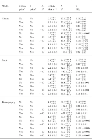
Results from these analyses are shown in Table3.

3.4.2 Bou´e model

We investigate the system using the Bou´e model, following the same methodology outline for the Hirano model. We again adopt a constraint of zero drift in the barycentric ve-locity owing to lack of evidence to the contrary. Applying the stellar radius constraint led to increases inMs, Rs,ρs, Mp,Rp, andTeff, but in several cases these parameters were unphysical. There was also no substantial improvement in fit when applying the radius constraint, and we therefore elected not to do so. We also adopted a circular solution as there was no evidence for a significantly eccentric orbit. In this we match our choice of constraints for the Hirano model, which is encouraging as it again shows that the two mod-els are broadly consistent in their exploration of parameter space.

Initial tests without a prior onvsinIsalso produced re-sults consistent with those found using the Hirano model, in-cluding the crescent-shaped degeneracy betweenvsinIsand λwith a preference for positiveλ, though the stellar rotation velocity was found to be even slower at 0.4+0−0..51km s

−1

Figure 12.Upper panel: a close up of the RM anomaly in the RV curve of WASP-76, after correcting for a correlation between FWHM and RV residuals, with the contribution from the Keple-rian orbit subtracted to better display the form of the anomaly. The two model fits are barely distinguishable. No prior on the impact parameter is applied. Lower panel: the residuals for the

two model fits. Legends for the two panels as for Fig.2.

λ0 =±90◦, the convergence statistics were again improved and the chains explored the expected minimum, but like the Hirano model tests the impact parameter remained lower than anticipated.

Applying a prior on the impact parameter, in the ab-sence of the vsinIs prior, showed that the chains favoured the positive minimum, but with sizeable uncertainty on λ and a slow rotation velocity. When we apply priors on both impact parameterand vsinIs, we found results consistent with the Hirano model equivalents.

3.4.3 Doppler tomography

We adopted constraints ofe= 0 and ˙γ= 0, but left the stel-lar mass and radius freely varying, in order to be consistent with our analyses using the Hirano and Bou´e models.

As anticipated, using the DT method substantially re-duced the degeneracy between vsinIs and λ, though it did not, for this system, remove it completely (see Fig.14). DT again favoured the positive minimum, though more strongly than the other two models, and again returned a more slowly rotating star than anticipated. Adding a prior on vsinIs, however, produced different behaviour than shown

previ-Figure 13.Map of WASP-76 time series CCFs with the model

stellar spectrum subtracted, for the case with no application of a

vsinIsprior from spectral analysis. The trajectory of the planet

signature is difficult to determine owing to the slow rotation of the host star. The planetary signal appears to bleed outside the area of the plot denoting the stellar boundaries, perhaps indicating

that this method is underestimatingvsinIs. Legend as Fig.4.

ously. With DT, adding a prior onvsinIsforced the chains into the negative minimum, with no bimodal distribution observed, though once again the impact parameter strongly disagreed with the value from the discovery paper and im-plied a central transit.

If we impose a prior on the impact parameter using the value from the discovery paper, then in the absence of a prior onvsinIs we again find that the chains favour the positive minimum inλ, irrespective of the value ofλ0. We also find a faster value of vsinIs than was returned by either the Hirano or Bou´e models for the same combination of priors, though the values are consistent to 1σ. If we add the prior on vsinIs then the results remain consistent, but the 1σ uncertainties are reduced in magnitude, particularly forλ which also moves closer towards a value that implies a polar orbit.

3.4.4 A possible polar orbit?

s

Table 3.A summary of the results obtained during our investigation of the WASP-76 system. We explored different combinations of

Gaussian priors onvsinIs andb, while allowing the stellar parameters to float freely and fixinge= 0 and ˙γ = 0. We also explored

the effect of varyingλ0 between different local minima. We found that the application of a prior onbleads to a positive solution forλ,

irrespective of the value ofλ0. Behaviour in the presence of a prior onvsinIsvaries with the choice of model, but does force the chains

to limit themselves to a single minimum inλparameter space.

Model vsinIs b λ0 vsinIs λ b

prior? prior? /◦ /km s−1 _/◦ _/R

s

Hirano No No 0.7+0₋₀._.27 37.6₋+31₅₂._.4₅ 0.11+0₋₀._.11₀₈

Yes No 2.2±0.4 73.4+6−151.2.2 0.03

+0.04

−0.02

Yes No 90 2.0±0.4 76.5+3₋₅._.8₁ 0.09+0₋₀._.04₀₆

Yes No −90 2.2±0.4 −76.8+4−3..55 0.02

+0.02

−0.01

No Yes 0.7+0−0..52 41.1

+25.0

−50.1 0.130±0.003

No Yes 90 0.7+0₋₀._.15 42.1₋+24₄₉._.0₉ 0.13+0₋₀._.01₀₁

No Yes −90 0.7−+00..52 41.8

+24.7

−50.4 0.130

+0.003

−0.004

Yes Yes 1.9±0.3 74.8+4₋₅._.0₂ 0.130+0₋₀._.001₀₀₃

Yes Yes 90 1.9±0.3 74.8+4−5..25 0.130

+0.001

−0.002

Yes Yes −90 2.1±0.4 −76.9+4−3..53 0.02

+0.02

−0.01

Bou´e No No 0.4−+00..51 34.7

+36.8

−64.9 0.10

+0.10

−0.08

Yes No 2.2±0.4 82.2+2−164.4.8 0.02

+0.02

−0.01

Yes No 90 2.2±0.4 82.9₋+1₂._.9₆ 0.03±0.02

Yes No −90 2.2±0.4 −82.9+2−1..27 0.01±0.01

No Yes 0.4₋+0₀._.2₁ 37.1+27_−52..7₉ 0.13+0₋₀._.01₀₁

No Yes 90 0.4+0−0..31 34.6

+29.3

−52.9 0.13

+0.01

−0.01

No Yes −90 0.4−+00..31 36.8

+27.8

−51.9 0.13±0.004

Yes Yes 2.0+0₋₀._.3₄ 70.0+7₋₁₁.0_.6 0.13±0.01

Yes Yes 90 2.0±0.3 70.2−+611.6.7 0.13±0.003

Yes Yes −90 2.1±0.3 69.6₋+6₁₀.8_.6 0.13±0.01

Tomography No No 1.2+0−0..96 69.3

+10.2

−26.7 0.11

+0.09

−0.06

Yes No 2.1±0.3 −77.4₋+3₂._.6₉ 0.01±0.01

Yes No 90 2.2±0.3 77.3−+32..79 0.01±0.01

Yes No −90 2.1±0.3 −77.2+4−3..00 0.01±0.01

No Yes 1.1₋+0₀._.5₄ 64.6+10_−23..0₆ 0.13+0₋₀._.01₀₁

No Yes 90 1.1+0−0..54 64.1

+10.0

−25.2 0.130±0.003

No Yes −90 1.1±0.5 66.4₋+9₂₁.1_.1 0.13±0.01

Yes Yes 1.9±0.3 76.5+3−4..44 0.130±0.002

Yes Yes 90 1.9±0.3 77.7−+33..19 0.130±0.003

Yes Yes −90 1.9±0.3 76.4₋+3₄._.4₄ 0.129±0.003

In the absence of a prior on rotation, our modelling of the RM effect using any of the three methods gives a value sig-nificantly slower than this, at ∼ 1 km s−1. Yet inspection of both the CORALIE and HARPS spectra reveals visible rotation (see Fig.15), and the full width at half-maximum (FWHM) of the spectra are greater than for stars with sim-ilar (B− −V) colour, such as WASP-20. This would suggest that the star is indeed oriented close to edge-on, rather than the pole-on orientation suggested by the slow rotation ve-locity returned by our MCMC chains.

We therefore consider the possibility that the orbit is

oriented at close to |λ| = 90◦, with a transit chord such that the path of the planet is almost parallel to the stellar rotation axis. This solution is consistent with the path of the planetary ‘bump’ through the stellar line profile in Fig.13, which shows little movement in velocity space. To explore this possible system configuration, we carried out additional analyses both with and without a prior onvsinIs, this time forcing the MCMC chain to adoptλ = ±90◦ throughout. Note that these analyses used the constraints ofe= 0 and

˙

0.00 0.02

−50 0 50 0

2 4 6 8 10

0.0 0.1 0.2

v sin i

*

/ km s

−1

λ / deg

. .

. .

0.0 0.1

−50 0 50 0

2 4 6 8 10

0.0 0.1 0.2

v sin i

*

/ km s

−1

λ / deg

. .

. .

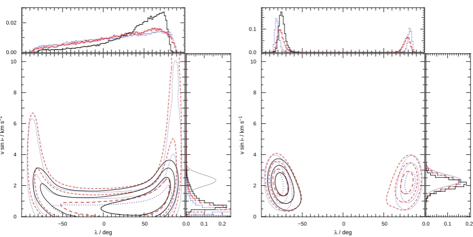
Figure 14.The posterior probability distributions invsinI−λparameter space for our analyses of WASP-76. Legend as for Fig.5. No

prior on impact parameter is applied. Left: results without a prior onvsinIs. DT fails to break the degeneracy that arises betweenvsinIs

and λas a result of the low impact parameter of the transit chord, although the length of the largevsinIs, large|λ|tails is strongly

reduced. Right: results with a spectral analysis applied tovsinIs. As with WASP-61, the degeneracy between solutions with (iorb,λ)

and (iorb−π,−λ) leads to a bimodal distribution when using the Hirano and Bou´e models. Unlike that system however, the bimodality

is on a chain-by-chain basis; each individual chain concatenated in our final MCMC chain is well converged on to either the positive or

negativeλsolution. DT succeeds in breaking this degeneracy, with all chains produced using that model converging at the negativeλ,

retrograde solution. However, there is little reduction in the size of the distribution compared to the Bou´e and Hirano models.

radius, as before. We present these results in Table4 and Fig.12.

We found that when applying the Bou´e model, the MCMC chains took approximately twice as long to converge as when applying the Hirano model. The source of this diffi-culty with convergence is uncertain, but seems to be related to the ratio betweenσBoueandvsinIs. Large steps in the lat-ter that explore rapidly rotating solutions lead to unphysical values of this ratio, such that the step fails. This restricts the set of possible solutions to a more limited area of parameter space, such that a larger percentage of possible steps lead to poor solutions, and thus convergence of the chain proceeds more slowly.

The three analysis techniques generally produced con-sistent results. In the majority of cases, we found that the value forbreturned by the chains was in agreement with the discovery paper; the exceptions to this were the cases with λ0=−90◦and thevsinIsprior only. With the rotation prior

inactive, the only case to be consistently in agreement with

predictions across all three techniques was the case with b prior also inactive, andlambda0 = 90◦; in the other cases, the stellar rotation was generally slower than the spectral analysis result (as noted in previous sections).

These results lend some small support to the hypothesis of a polar orbit, as we note that in the case of neither prior being applied the results were consistent with both spectral analysis and the discovery paper.

3.4.5 A poorly constrained system?

WASP-76 seems to represent a similar case to WASP-1 ( Al-brecht et al. 2011): a low impact parameter, combined with a poor SNR for the RM effect, leading to a weak detection. Here though, we find a three-way degeneracy between λ, vsinIs, andbthat can only be broken through the applica-tion of appropriate Gaussian priors.

Our results show tentative support for a strongly mis-aligned orbit. Applying a prior on stellar rotation or on the impact parameter produces results that suggest strong mis-alignment, particularly when using the DT method. Forcing the system to adopt a polar orbit, or using a polar orbit as the initial condition, reveals that this is a plausible option for the system’s configuration, though there is still substantial ambiguity in the precise orientation of the planet’s orbit.

s

Table 4.A summary of the results obtained while investigating a potential polar orbit for WASP-76. We fixedλ=±90◦, and explored

different combinations of Gaussian priors onvsinIsandbwhile allowing the stellar parameters to float freely, and fixinge= 0 and ˙γ= 0.

Model vsinIs b λ0 vsinIs λ b

prior? prior? /◦ _{/km s}−1 _/◦ _/R

s

Hirano Yes No 90 2.2±0.4 90 (fixed) 0.06+0−0..0403

−90 2.2±0.4 −90 (fixed) 0.01+0₋₀._.02₀₁

Yes 90 2.0±0.4 90 (fixed) 0.13±0.02

−90 1.6−+00..64 −90 (fixed) 0.13

+0.003

−0.10

No No 90 1.0+4_−0..₉6 90 (fixed) 0.11+0₋₀._.12₀₉

−90 0.2−+00..92 −90 (fixed) 0.05

+0.11

−0.04

Yes 90 0.8−+00..76 90 (fixed) 0.13±0.02

−90 0.1₋+0_0..3₁ −90 (fixed) 0.13±0.02

Bou´e Yes No 90 2.2±0.4 90 (fixed) 0.03±0.02

−90 2.2±0.4 −90 (fixed) 0.01±0.01

Yes 90 2.1₋+0_0..3₄ 90 (fixed) 0.130±0.001

−90 1.8±0.3 −90 (fixed) 0.130±0.001

No No 90 1.5+5−1..63 90 (fixed) 0.10

+0.15

−0.08

−90 0.3+1₋₀._.8₃ −90 (fixed) 0.07+0₋₀._.10₀₅

Yes 90 0.3−+00..43 90 (fixed) 0.130±0.001

−90 0.1−+00..21 −90 (fixed) 0.130±0.001

Tomography Yes No 90 2.2±0.3 90 (fixed) 0.09±0.03

−90 2.3±0.4 −90 (fixed) 0.01±0.01

Yes 90 2.2±0.3 90 (fixed) 0.130±0.002

−90 1.8±0.3 −90 (fixed) 0.13±0.01

No No 90 1.6±0.8 90 (fixed) 0.12+0−0..0905

−90 0.1+1₋₀._.0₁ −90 (fixed) 0.05+0₋₀._.11₀₄

Yes 90 1.3−+00..67 90 (fixed) 0.130±0.001

−90 0.01±0.01 −90 (fixed) 0.130±0.002

3.5 WASP-78

WASP-78 b (Smalley et al. 2012) is large-radius, low-density hot Jupiter that orbits its host star every 2.2 d in a circular orbit. From the CORALIE RV data in the discovery pa-per, the orbit appears to be circular, and such a solution is adopted therein, but the authors state that additional RV data is required to pin-down the eccentricity. Spectral analysis shows that the host star is of spectral type F8, with Teff = 6100±150 K, vmac = 3.5±0.3 km s−1, and vsinIs= 7.2±0.8 km s−1.

We obtained new photometry using EulerCam, in both theIandRbands, of transits on 2012 November 2 and 26, respectively, which we combine with the discovery photom-etry from WASPSouth and TRAPPIST. TheR-band light curve shows clear modulation, almost certainly as a result of the presence of star-spots or related stellar activity fea-tures, as this modulation is not replicated in theI-band light curve (Fig.17). Our HARPS spectroscopic transit observa-tions were made simultaneously with theI-band EulerCam observations, and used in conjunction with spectroscopy

from CORALIE. Analysis of the HARPS spectra provides vmac= 4.85 km s−1, andvsinIs= 6.63±0.16 km s−1.

3.5.1 RM modelling

As with the other systems in our sample, we find no evidence of a long-term barycentric velocity trend, and set ˙γ= 0. We also find little difference in behaviour or results between the two models; the following discussion is applicable to both.

0.6 0.65 0.7 0.75 0.8 0.85 0.9 0.95 1 1.05

5538 5538.2 5538.4 5538.6 5538.8 5539

Normalised flux

λ (Å)

Figure 15.The line profile of the FeIline at 5538.517 ˚Aof

WASP-76 A, as observed with HARPS (black, solid line). Overlaid are

models for two different values ofvsinIs: 2.33 km s−1, the

spec-troscopic value (red, dashed line), and 1.0 km s−1, on the order of

the results returned by the RM models (blue, dotted line). While the red model fits the observed line profile well, the blue model is both deeper and more narrow.This indicates that the host star is rotating more quickly than the RM models are able to account for if the planet is on a non-polar orbit.

Figure 16.As for Fig.12for the RM effect of WASP-76 in the

case where an orbit parallel to the stellar rotation axis,λ= 90◦,

was forced.

Figure 17.Upper panel: newly acquired EulerCam observations

of two separate transits of WASP-78 b, with best-fitting MCMC

transit models. The two light curves have been offset by 0.015 mag

for clarity. The lower, red data are theR-band light curve of the

transit on 2012 November 26. The upper, blue data are theI-band

light curve of the transit on 2012 November 2. The signature of

stellar activity is detected in theR-band, with structured

varia-tion in the light curve. There is also some evidence for activity in

theR-band light curve, but this is less conclusive. Lower panel:

residuals of the fits of the data to the best-fitting transit models.

The stellar activity signature from theR-band light curve is more

clear in the residuals.

the method of Lucy & Sweeney (1971) reveals that they are not significant. Comparing eccentric and circular solu-tionswith no other constraints applied, we find that varia-tions in physical parameters are within the 1σuncertainties. We thus choose to force a circular orbit as it provides the most plausible solution; the phase coverage of the HARPS data is insufficient to truly constrain any small eccentric-ity that might be present, and the pre-existing CORALIE RV data cannot provide a firm conclusion regarding circu-larity (or otherwise). We also note that hot Jupiters with Mp≈1 MJupare generally observed to have zero (or small) eccentricity (Anderson et al. 2012).

Application of the stellar radius constraint to a circular orbit increases the reported stellar mass, and also leads to an increased value of Teff and a lower impact parameter. Our results in this scenario agree very well with those from Smalley et al.(2012), as expected; the host star is both too massive and too large, and inconsistent with both spectral analysis of both the existing CORALIE spectra and our new HARPS data. Conversely, if the planet’s orbit is allowed to be eccentric (against the evidence), then adding the stellar radius constraint decreases the mass of both bodies, and significantly decreases their radii.

s

Figure 18.Upper panel: the RV curve of WASP-78, phase folded

using the best-fitting ephemeris. HARPS data are denoted by solid circles, CORALIE data by open triangles. The best-fitting barycentric velocity for each set of data has been subtracted. Overplotted are models for a circular solution (solid, black line), a

model withe= 0.05 (dashed, red line), and a model withe= 0.6

(dotted, blue line). We adopt the circular solution in our final results, as the high eccentricity solution is clearly incorrect, and there is insufficient evidence for a small eccentricity. Lower panel: the residuals for the two model fits. Data are colour-coded ac-cording to the model being fit.

do not apply a prior using the spectroscopic vsinIs. Our chosen solution is therefore a circular orbit with no long-term velocity trend, and no application of the constraints on vsinIsorRs. The full set of results is shown in Table5, but the alignment angles found by the Hirano and Bou´e models are consistent with each other, and withλ= 0, implying a well-aligned orbit. We do however find that the Bou´e model produces a slower rotation velocity, as we found for all of the previous systems, in this case inconsistent with the spectro-scopic value. This cannot, however, be as a result of a poorly constrained impact parameters; the results in Table5show that the impact parameter returned by the Bou´e model is in agreement with the results from other models, and has similar 1σuncertainties.

The form of the best-fittingting models are very similar in Fig.19, as they were for WASP-76 (the other system with a low signal-to-noise anomaly), although in this case there are far fewer data during the transit.

Our selected solutions are taken from runs for which no

Figure 19.Upper panel: a close up of the RM anomaly in the

RV curve of WASP-78, with the contribution from the Keplerian orbit subtracted to better display the form of the anomaly. Lower panel: the residuals for the two model fits. Legends for the two

panels as for Fig.2.

prior was applied tovsinIs,e= 0, ˙γ= 0, and no constraint was applied to the stellar radius.

3.5.2 Doppler tomography

We apply the same set of constraints to our tomographic MCMC analysis (Fig.20) as for the RM modelling runs. We find that all parameters are in agreement with the results from the Hirano model and the case in which no RM mod-elling is carried out, and that all parameters exceptvsinIs are in agreement with the Bou´e model results, though we note that the disagreement there originates with the Bou´e model rather than DT. Unlike for some of the other systems studied herein, we find a roughly factor of 2 improvement in the precision of our alignment angle measurement over the RM modelling methods when using tomographic analysis (see Fig.21and Table5).