Bayesian structural identification of a long suspension bridge considering temperature and traffic load effects

Structural Health Monitoring 1–14

ÓThe Author(s) 2018 DOI: 10.1177/1475921718794299 journals.sagepub.com/home/shm

Bayesian structural identification of a

long suspension bridge considering

temperature and traffic load effects

Andre Jesus

, Peter Brommer

, Robert Westgate

, Ki Koo

,

James Brownjohn

and Irwanda Laory

Abstract

This article presents a probabilistic structural identification of the Tamar bridge using a detailed finite element model. Parameters of the bridge cables initial strain and bearings friction were identified. Effects of temperature and traffic were jointly considered as a driving excitation of the bridge’s displacement and natural frequency response. Structural identifi-cation is performed with a modular Bayesian framework, which uses multiple response Gaussian processes to emulate the model response surface and its inadequacy, that is, model discrepancy. In addition, the Metropolis–Hastings algorithm was used as an expansion for multiple parameter identification. The novelty of the approach stems from its ability to obtain unbiased parameter identifications and model discrepancy trends and correlations. Results demonstrate the applicability of the proposed method for complex civil infrastructure. A close agreement between identified parameters and test data was observed. Estimated discrepancy functions indicate that the model predicted the bridge mid-span dis-placements more accurately than its natural frequencies and that the adopted traffic model was less able to simulate the bridge behaviour during traffic congestion periods.

Keywords

Bayesian inference, multiple response Gaussian process, Metropolis–Hastings, long suspension bridge, model discrepancy

Introduction

Critical civil infrastructure, such as long suspension bridges, represents a capital investment from commu-nities and local governments. Therefore, its serviceabil-ity fully justifies dedicated long-term monitoring systems. structural health monitoring (SHM)1concerns the design, deployment, maintenance of structural monitoring systems and subsequent data interpretation. Relative to data interpretation, the actual structural behaviour is often grossly misinterpreted when com-pared against the input–output relation of a physics-based computer model.2 In other words, structural identification (st-id) is very susceptible to uncertainties. These uncertainties stem from experimental and con-ceptual factors, such as the high heterogeneity of moni-tored data or model discrepancy, that is, modelling assumptions and simplifications.

Several probabilistic st-id methodologies,3,4 such as Kalman filters5 or fuzzy logic,6 have been used to address these uncertainties. Another example is Bayesian methods, which have been introduced to the SHM community by Sohn and Law,7 Beck and

Katafygiotis,8 and Beck and Au.9 Unfortunately, the frameworks proposed by these authors are not well sui-ted to address the confounding influences due to envi-ronmental (temperature, wind) and operational (traffic, pedestrians) actions.10–13 Recently, Behmanesh et al. presented a hierarchical Bayesian framework,14,15

1_{Civil Research Group, School of Engineering, The University of}

Warwick, Coventry, UK

2_{Warwick Centre for Predictive Modelling, School of Engineering, The}

University of Warwick, Coventry, UK

3

Centre for Scientific Computing, The University of Warwick, Coventry, UK

4

Atkins Global, Cambridge, UK

5

College of Engineering, Mathematics and Physical Sciences, The University of Exeter, Exeter, UK

Corresponding authors:

Andre Jesus, Civil Research Group, School of Engineering, The University of Warwick, Coventry CV4 7AL, UK.

Email: [email protected]

Irwanda Laory, Civil Research Group, School of Engineering, The University of Warwick, Coventry CV4 7AL, UK.

which, in the absence of noise or model discrepancy, accurately identifies parameters subjected to external actions.16

Thus, in addition to environmental/operational effects, model discrepancy is the main challenge hinder-ing these methodologies. Accordhinder-ing to the principle of maximum entropy,17 this source of uncertainty has recurrently been assumed as a zero-mean uncorrelated Gaussian.18–22Such assumption is reasonable as a con-servative upper limit, but it brings considerable short-comings. Namely, it introduces parameter inference bias and negates the possibility of finding patterns and correlations, which are vital for model updating and performance assessment. Authors, such as Goulet and Smith3 or Papadimitriou and Lombaert,23 have high-lighted the benefits of weakening such assumptions for st-id and measurement system design, respectively.

The main alternative to physics-based models is an interpretation with data-based models,24,25which is not bound by physical laws and thus can approximate data patterns more efficiently without model discrepancy. Examples include clustering26 or Gaussian mixture27 models, which are used for damage identification using Bayesian inference. However, data-based models have a limited ability for extrapolation and thorough expla-nation of data trends. Finally, hybrid models gather both, a descriptive coherency of a structural system, and adaptability for identification of unusual data patterns.

Consequently, the current contribution applies a dif-ferent approach to the problem of st-id. The framework

under focus is a hybrid modular Bayesian approach (MBA) developed based on the method proposed by Kennedy and O’Hagan.28 Previous work by Jesus et al.29 highlighted an application of the MBA to a reduced-scale aluminium bridge (under temperature variation only). The work however was restricted to the identification of a single parameter. If model discre-pancy is approximated with a multiple response Gaussian process (mrGp), then probabilistic st-id in SHM is expected to improve. Therefore in this article, encouraged by the previous work, an expansion of the MBA using the Metropolis-Hasting algorithm for mul-tiple parameters identification is presented. This article also details the first application of the method to a full-scale structure, the Tamar long suspension bridge, under temperature and traffic loading.

Enhanced MBA

In this section, a short summary of the MBA and rele-vant details of its enhancement for multi-parameter identification are presented. For the remainder of this work Table 1 is to be used as a nomenclature table.

The original MBA formulation was developed for a single response case,28,30 that is, only considering pre-dictions of one model output function. Arendt et al.31 proved that, unless under some specific conditions, the single response case fails to identify the true structural parameters. Instead, a multiple response formulation which allows for a more informative data model has been proposed.32

Table 1. Table of notation.

Nomenclature applicable to the MBA

e Observation error Xe Experimental dataset ofX

d Discrepancy function Xm Model dataset ofX

X Design variables Xe Dataset of measured response

u Structural parameters Ym Dataset of simulated response

f mrGp hyperparameters Θm Model dataset ofu

Nomenclature applicable to the Tamar bridge

tc Cables temperature eiMC Main cables initial strain

tS Shaded elements temperature eiSC Stay cables initial strain

tL Lighted element temperature Kd Bearings stiffness

mt Traffic mass

Tamar bridge natural frequencies labels

‘L’ Lateral ‘S’ Symmetric

‘V’ Vertical ‘A’ Asymmetric

‘T’ Torsional ‘SS’ Side span

MBA Modular Bayesian approach MCMC Markov chain Monte Carlo

TPS Total positioning system FE Finite element

mrGP: multiple response Gaussian process.

General workflow of the MBA

The MBA aims to solve an equation of model calibra-tion, which can be written as follows

Ye(Xe) =Ym(Xe,u) +d(Xe) +e ð1Þ

whereYe are observations, dependent on design vari-ablesXe;Ymare simulations of a model, dependent on the design variables and a vector of unknown structural parameters u; d(Xe) is a discrepancy function that translates the inadequacies between the model and the true process; and e is an observation error, which is assumed to follow a Gaussian distribution N(O,L). Equation (1) is analogous to the formulations of the classical and hierarchical Bayesian frameworks, although it features the design variablesXe to allow to consider temperature, wind, loads and other external effects which influence the structural response.

There are an infinite number of solutions of equa-tion (1). For different values of the parameters , there will always be a discrepancy function that matches that particular model instance with Ye_(Xe_{). However, the} goal is to calibrate the model with parameters set at their true valuesu and obtain a discrepancy function

which reflects the actual deficiencies of the model. By definition, a parameter is said to be trueu if set at a value which corresponds to its physical interpretation.

Finally, Bayes’ theorem can be used to update the belief on the structural parameters as follows

p(YjD) = R p(Dju)p(u)

p(Dju)p(u)du ð2Þ

wherep(ujD)is the posterior distribution of u,p(u) its prior,p(Dju) is the likelihood function based on equa-tion (1), and the denominator is called the marginal likelihood. Finally, D represents available simulated

fXm,Θm,Ymgand monitoredfXe,Yegdata. Note that Θm_{represents an input dataset used to build the} likeli-hood function, oppositely to the identified structural parametersu.

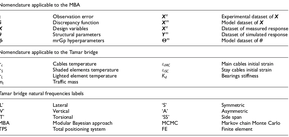
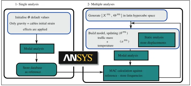
The MBA breaks the complete process described above into four modules, hence the name MBA. For a flowchart of the algorithm, see Figure 1. Inmodules 1 and 2, the model response surface and the discrepancy function are fitted by statistical models, known as mrGp, whose parameters (hyperparametersf) have to be estimated. See a definition in the Supplemental Material. The main assumption associated with fitting

a mrGp to a process is for its behaviour to be smooth and continuous.

In module 3, the estimated hyperparameters of the mrGps become fixed and are used to set up a global data model, the likelihood function, that explains both simulations and observations for a set of given struc-tural parameters u. The posterior distribution is esti-mated through equation (2). The finalmodule 4predicts the observed process, by updating the mrGps previ-ously determined with the posterior probability density function (PDF) ofu.

Note that such a modular separation will greatly reduce the computational effort required to solve equa-tion (1), comparatively to other Bayesian frameworks. It implies that the uncertainty effects are not considered fully. As a drawback, identification of true parameters is more challenging. However and as established by Arendt et al., considering multiple responses consider-ably improves the identifiability of the MBA.

The next section presents an enhancement over the above described formulation.

Markov chain Monte Carlo sampling of posterior

distribution

Previous implementations of the MBA are limited to identification of a single structural parameter. This sec-tion discusses a Markov chain Monte Carlo (MCMC) routine which allows to identify multiple parameters with the MBA. The Gauss–Legendre has been used for the single-parameter case, whereas our implementation includes a routine based on the Metropolis–Hastings (MH) algorithm.33,34 MCMC methods are commonly used to address multi-dimensional integrals which occur in fields such as Bayesian inference.9

Since the likelihood of the MBA is multivariate nor-mal and analytically untractable, numerical methods are required to perform its integration. The MH

algorithm is known to converge to a target distribution for an increasing number of samples. Specifically, the target distribution has been assumed as symmetric and sampled with a 3000 burn-in period for a total of 100,000 samples. A standard multivariate normal dis-tributionN(O,I) was assumed as a proposal distribu-tion. This choice is reasonable, because the input data are standardised for numerical convenience. Finally, obtained samples were post-processed in order to ana-lyse the likelihood PDF and estimate the marginalised posterior.

Although it is acknowledged that the MH algorithm has its limitations, and an alternative such as the adap-tive Metropolis algorithm would be more suitable,35the aim is to showcase the potential of the MBA to identify multiple parameters and motivate further develop-ments. In the following sections, its performance shall be illustrated with an application to the Tamar long suspension bridge.

Tamar bridge experimental and simulated

dataset

This section presents the Tamar bridge’s SHM system, the monitored data under consideration and the finite element (FE) model developed to study its behaviour.

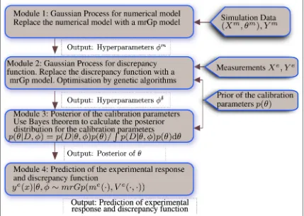
Tamar bridge is a 335-m-long suspension bridge, built in 1959 and reconstructed between 1999 and 2001, where a larger side deck and stay cables have been added, see Figure 2 for a reference. Two long-term monitoring systems have been installed and several localised expeditions have been carried out through time for reliability assessment.

In addition, an FE model was developed by Westgate37 to study environmental and operational effects on its structural performance. It is worth men-tioning the following excerpt ‘In fact, Tamar Bridge has so far presented a challenging case study for model

calibration, lending support to the view that no single model provides a perfect representation of a structure when matched to provided experimental data’.38

On the basis of the present methodology and data/ model, three key properties relevant for stake holders will be estimated. One is the friction in the thermal expansion bearings of Saltash tower, which can lead to deck cracks and further structural anomalies. The remaining two properties are the initial strain in the main and stay cables of the bridge. The initial strain is defined as the strain relative to when the bridge cables have been installed initially, that is, containing all the load-history that the cables have supported since instal-lation. Its increase could indicate internal damage, such as broken wires, corrosion, cracks and wear.

Monitored data and post-processing

It is important to establish which design variables are relevant to study Tamar bridge’s dynamic behaviour. A study from Cross et al.39indicates that traffic, tempera-ture and wind have the most influence on Tamar bridge natural frequencies, by decreasing order of relevance. However, this study will be limited to the effects of traf-fic and temperature.

In the absence of the above information, a normal procedure would include the following:

Monitor the structural behaviour for a certain period of time, preferably at least for a year period;

Analyse existent correlations between environmen-tal/operational effects and the structural output, displacements, vibration data, and so on;

Select the effects which have the highest influence on the structural output and consider them during the modelling process.

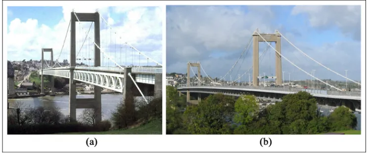
Several sensors have been installed through time on Tamar bridge, but for the purpose of this study, we considered data which were monitored from a set of accelerometers, a total positioning system (TPS) reflec-tor and thermocouples, which are shown in Figure 3. The available data also include vehicle counts from toll gates of the Plymouth side.

The monitoring period ranged from May 2009 to March 2010, where synchronised temperature, traffic and modal data were found to be richer. Furthermore, a year time-frame was assumed as a good reference for calibration/validation of the FE model, since it covers seasonal variations. Relevant post-processing opera-tions will now be detailed.

First, the natural frequencies of the structure were determined with a stochastic subspace identification (SSI) technique,40based on available acceleration data. Specifically, at each half-hour, 10-min acceleration recordings were post-processed to determine the natu-ral frequencies and mode shapes of the infrastructure. Second, displacements at the middle span of the bridge in three directions, vertical, East and North, were obtained from the TPS.

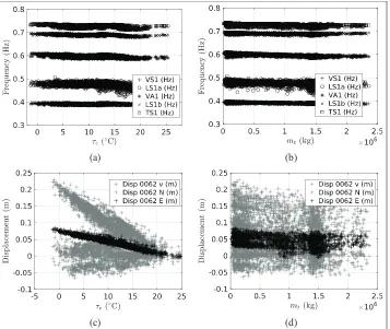
After the above-mentioned operations, a 2419 points dataset was obtained, which is visualised in Figure 4. Visible trends indicate linear correlations, except for the traffic/displacement relation in Figure 4(d). Therefore, a linear correlation function (or kernel) was assumed for the mrGps that fit the discrepancy function and the FE model.41 Furthermore, the zero displacements at highest temperatures in Figure 4(c) and (d) occur because the data have been offset relative to the highest peak of temperature3traffic load. Frequency labels follow the convention: ‘L’ is a lateral mode shape, ‘V’ is vertical mode shape, ‘T’ is a torsional mode shape, ‘TRANS’ is a longitudinal translation mode, ‘S’ is

symmetric, ‘A’ is asymmetric, ‘SS’ is side span and the numbers are their relevant order.

For future reference, it is worth mentioning some rel-evant information related to the bridge main and stay cables. Namely, the main suspension cables are made from 31 locked coil wire ropes, each 60 mm in diameter, and the overall diameter of the main cable is 380 mm, resulting in a cable cross-sectional area of 882.36 cm2. The stay cables indicated in Fig. 3 have areas of 87.01 cm2 for S2 and P2 (110 mm diameter strands) and 70.74 cm2 for the remaning cables (102 mm dia-meter strands).

Modelling of thermal and traffic effects

In this section, Tamar bridge FE model will be briefly described, along with to-be-identified structural para-meters, and modelling aspects of its dynamic behaviour in the presence of traffic and thermal variations.

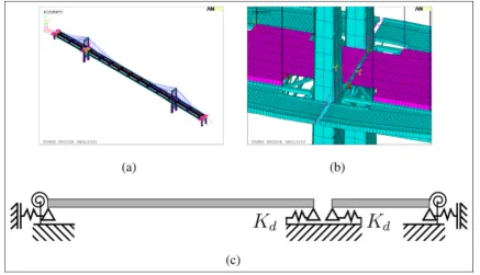
The FE bridge model has been developed using ANSYS Parametric Design Language (APDL) source code42 and consists of approximately 45,000 elements, from which expansion joints have been modelled with linear spring elements, truss members with fixed-rotation beams, deck/towers with shells and the cables and hangers with uniaxial tension only beam elements.

First, it is important to discriminate the three para-meters which will be identified. One is the stiffness of linear springsKd, as seen in Figure 5(b) and (c), which represents friction in the thermal expansion bearings of Saltash tower. The remaining two parameters are the initial straineiin the two main and 16 stay cables of the bridge.

For each cable type (main or stay), the initial strain is assumed constant along the cable length and across all cables. The Young’s modulus of the cables was assumed as 155 GPa, and the initial straineiaffects the axial tensile force N of the cables according to trivial constitutive laws, that is,N=EcAcei, whereEc,Ac repre-sent the cables Young’s modulus and cross-sectional area, respectively. It is known that the simulated natu-ral frequencies are sensitive to the cables initial strain parameters, as noted in Westgate and Brownjohn37 analysis. In turn, the mid-span displacements are sensi-tive to the stiffness of the thermal expansion gap, as shown in Westgate et al.38

Second, after having detailed the model parameters, it is now necessary to highlight how temperature effects have been considered. For the present work, a regres-sion was used to establish a simplified relation between temperature trends of the truss, deck, and cable

(a) (b)

(c) (d)

temperatures of the bridge (sensor location can be seen in Figure 3). Subsequently, temperature effects are con-sidered as a static steady-state thermal analysis, with three different temperature sets: shaded elements, which represent the truss structure under the deck; the elements that represent suspension cables; and other lighted elements excluding cables. Monitored data of these parts have been used to develop the regressive model, as can be seen in Figure 6.

Thus, the relation between the temperatures of the shaded, lighted and cable groups is

tS= 0

:433tc+7:877 tc.15 tc tc<15

ð3Þ

tL= 1

:544tc8:798 tc.15 tc tc<15

ð4Þ

where tc, tS and tL represent the temperature in the cable, shaded, and lighted elements, respectively.

It must be stressed that the linear relations of equa-tions (3) and (4) will only be applied when tc.158C, otherwise to be applied as a uniform temperature tc across all elements. This is interpreted as a notable change of cable temperature, where the temperature trends of the bridge fork.

Third, the effects of traffic load are also detailed. The traffic is assumed as a set of distributed mass points, evenly spread longitudinally across the bridge deck, and asymmetrically in the lateral direction. The

average number of vehicles on the bridge in the tolled direction can be assumed as approximately 1/43rd of the available half-hourly count. Hence, traffic effects were monitored as a function of a half-hourly total mass mt, which was retrieved from the available toll-gate count. In the FE model, the total mass is being fractioned into an half-hourly on bridge mass ms, as ms=mt=43.

Figure 5. Tamar bridge FE model and detail of imposed constraints simulated as linear spring elements. (a) Perspective view, (b) expansion gap at Saltash tower and (c) bridge boundary conditions diagram.

Figure 6. Assumed temperature relations between cable, shaded and lighted groups for Tamar bridge FE model and associated monitored data.

Finally, and gathering all the above-mentioned information, the simulations of the FE model have been performed in a Latin hypercube space, where values of temperature, traffic mass, and structural parameters were uniformly generated and the corresponding natu-ral frequencies/displacements stored. A flowchart of the whole process is shown in Figure 7. First, a single modal analysis was run with default values of structural parameters and without traffic or temperature loading. In the second phase, multiple analyses were run for each combination of the input dataset Xm and Θm_. Finally, the natural frequencies/displacements of each run were classified and stored using the modal assur-ance criterion (MAC) with a fit of at least 80 %.

Parameter identification and discrepancy

function prediction

MBA input dataset

Table 2 presents a summary of all the MBA input data, and the to-be-identified structural parameters

u=feiMC,eiSC,Kdg. The mean and correlation functions of the mrGps are set as a polynomial regression

H() =1 and a linear correlation, respectively. Prior information of the structural parameters is considered as a uniform PDF, bounded by the intervals where the dataset ½Xm_{,Θhas been generated. The lower bounds}

of the intervals were chosen to truncate non-physical values, whereas the upper limits are based on heuristics and reference values from previous literature.

In order to sample the likelihood PDF with the MH algorithm, four Markov chains have been generated, with a standard multivariate normal distribution set as the proposal distribution. Trace plots of accepted sam-ples are shown in Figure 8, and their acceptance ratio was 39%.

Prediction of model discrepancy

Beforehand, it is important to predict a discrepancy function, whose information can be used to update the model, or added to the model output to compensate for inevitable modelling inadequacies. In the current section, some of the obtained discrepancy function pre-dictions will be presented and commented. Since the outputs depend of temperature/traffic and mrGps are used for visualisation, the results assume the form of three-dimensional (3D) statistical response surfaces, that is, a mean 3D surface and a prediction interval cloud. However, for the sake of clarity, the prediction intervals surrounding the mean surface have been omitted. Finally, it is important to mention that when the predictions of the model agree more closely to the monitored data, for example, because the model has

Figure 7. Simulation flowchart.

Table 2. MBA input dataset for Tamar bridge.

Description

u Initial strain of maineiMCand stay cableseiSCand stiffness of linear springs at thermal expansion gapKd Xe Bridge cable temperature and total mass due to traffic load from Plymouth-to-Saltash direction

Ye Natural frequencies determined by SSI and mid-span displacement from TPS ½Xm,Θ combination set of½tc,mt,eiMCeiSCKdgenerated in a Latin hypercube space with

been fine-tuned and updated continuously, the closer the discrepancy function will be to a zero-mean uncor-related Gaussian.

A first example of the mean discrepancy function of the natural frequencies of the Tamar bridge is shown in

Figure 9. The first thing to observe is that none of the mean surfaces is close to zero, and all display a corre-lated behaviour. As noted before, wind also affects the natural frequencies of the Tamar bridge, so it is plausi-ble to assume that the visiplausi-ble correlation is due to wind. Second, some patterns are visible in the lateral sway modes in Figure 9(a) and (d), where the discrepancy increases smoothly with traffic mass up to a localised peak at 1400 tonnes. Note that the same peak occurs, irrespective of temperature, which indicates that it depends only of the modelled traffic effects and predo-minantly during rushing hours. Thus, it is reasonable to assume that it occurs because our model does not consider traffic from the Plymouth to Saltash direction. Summarily, the results highlight the limitations of not considering a two-way traffic model and assuming an asymmetric distribution of traffic mass. Equipped with this information, an analyst could integrate it in its model predictions or carry out further updates.

Other example is shown in Figure 10, where the model discrepancy of the mid-span displacements is being predicted by the MBA. The results indicate a bet-ter performance, since the shown surface resembles a

Figure 8. Trace plot of identified structural parameters.

zero mean uncorrelated Gaussian, particularly visible for the displacement in the lateral North direction.

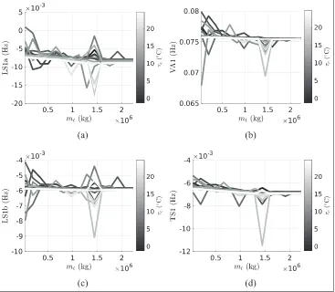
A final example is shown in Figure 11. The shown plots are equivalent to Figure 9(c) and (d) but with temperature in the abscissa. The model discrepancy for the two modes, LS1b and TS1, exhibits a temperature/ traffic interaction, since recurrent peaks occur at differ-ent temperatures and traffic values. It is important to always identify such patterns, and in which responses they become more proeminent, in order to ensure that the model predictions can be properly interpreted.

Validation of identified structural parameters

In this section, identified structural parameters are pre-sented and validated. Whereas the results of the previ-ous section are useful for model updating, identifying the true value of structural parameters is essential for

damage detection or reliability analyses. It should be noted that compared to the hierarchical Bayes from Behmanesh et al., the MBA is unable to capture the inherent variability of structural parameters. Therefore, note that the variance shown in the following results is associated with the estimation uncertainty of the parameters.

Sample histograms of the prior likelihood are played in Figure 12, and moments of the posterior dis-tribution are shown in equations (5) and (6). Since an uninformative prior has been assumed, the posterior distribution and the maximum a posteriori (MAP) are proportional/equivalent to the values obtained from the likelihood

E½ujD=

0:0012 0:0024 8:3290

2 4

3

5 ð5Þ

Figure 10. Prediction of the Tamar bridge mid-span (a) vertical and (b) Northern displacement discrepancy function for varying temperature (abscissa) and traffic (grayscale lines) conditions.

V½ujD=

0:25 0:081 168:47

0:081 1:17 519:28

168:47 519:28 5394863:84

2 4

3 53106

ð6Þ

Subsequently, validation of the identification of the stay cables and the thermal expansion gap will be pre-sented. Opportunely, expeditions and other estimates are available from past literature. The only exception are the main cables, which have never been monitored, and since its strains vary along its length, their results will be ommited.

The above estimates shall now be compared against an st-id confidence interval reported by Laory et al.44 and Goulet.45An estimate of the cables internal forces was obtained based on the initial strain MAP and the FE model predictions for each cable. Results are

displayed in Table 3. For the stay cable forces, there is a reasonable agreement between the two methodologies, since the MBA MAP falls near the upper limits of the model falsification (MF) confidence interval. However, for the stiffness of the thermal expansion gap, the MBA estimate is considerably less than the MF interval. A high value of this parameter would indicate that the bridge deck is prone to develop cracks. In order to investigate which estimate is closer to the true friction value, and to further analyse the stay cables behaviour, a comparison against monitored data will be detailed next.

The predicted stay cable forces are plotted along with monitored forces from existent strain gauge load cells, as shown in Figure 13. It is also important to stress that these monitored forces have not been used to estimate the posterior PDF. Both histograms have

(a) (b)

(c)

Figure 12. Inference of structural parameters: (a) main and (b) sway cables initial strain and (c) stiffness of thermal expansion gap.

Table 3. Identification of cable forces, stiffness of thermal expansion gap and comparison against model falsification.

kN kN kN/mm

Year SC (2) SC (1,3,4) Kd

(MF) [674, 4045] [548, 3289] [104_{, 10}11_]

(MBA) 3236 2631 8.32

been normalised in the coordinate axis by an estimate of probability density.

First, it can be seen that the P3S cable has three to four times larger forces, and as reported in Koo et al.,46 has a stronger dependency on temperature, than other stay cables. It is not certain why such behaviour occurs. Second, it can be observed that the posterior obtained by the MBA falls between the P3S and the other cables histograms. Two reasons might aid to clarify this result:

1. Since the parameter is assumed constant across all cables, its posterior distribution falls between the two other histograms, acting as an average value. 2. The offset might occur because the parameter

rep-resents an initial strain, that is, the strain relative to when the bridge cables have been installed on the bridge, and not relative to the strain existent when the strain gauge load cells have been installed.

Note that point number 1 assumes that the P3S cables force is genuine, in which case the posterior dis-tribution would have to be shifted towards lower values (since there are much more cables in the lower cable forces region). Thus, it is more plausible to believe that point 2 is the underlying reason for the posterior posi-tion, and that the values it indicates are closer to the true structural behaviour of the cables.

Finally, Battista et al.47 recorded temperature and extension data in the thermal expansion gap, starting 2 months after the timeframe of data used for the MBA identification, that is, in July 2010. Results from Battista’s work revealed that the gap extension against temperature is perfectly adjusted to a linear relation (see Figure 15 of the above work for clarification) and does not indicate any relevant frictional force. Hence, a lower value of stiffness, such as the one identified by the MBA, suggests a better agreement with in situ tests.

Conclusion

In this work, the MBA has been applied for st-id of the Tamar long suspension bridge. The methodology has been expanded to identify multiple structural para-meters, including the bridge’s cables initial strain and the stiffness of its thermal expansion gap. A detailed FE model of the bridge, on which environmental and operational effects were considered, has been calibrated and its performance has been assessed by a predicted model discrepancy.

Results suggest that

The developed methodology is able to identify mul-tiple parameters using the MH and a multi-dimensional Monte Carlo integration.

Compared against work from previous authors, the MBA provides an identification which agrees more reasonably with monitored data, particularly for the friction of the thermal expansion gap. This has been validated with in situ tests.

The current analysis is conditioned by the ability of its user to model environmental/operational effects. However, in contrast with other Bayesian meth-odologies, it is capable of performing st-id on large-scale infrastructure, highlighting trends and pat-terns of model discrepancy.

In general, the Tamar bridge FE model performs better at predicting the mid-span displacements than natural frequencies. In addition, the limita-tions of the developed traffic model and its interac-tions with temperature have been presented and discussed.

The calibrated FE model can be used as a reference baseline, for further investigations/health assess-ments, for example, damage detection.

In conclusion, the application of the MBA for st-id for large-scale civil structures has been comprehensively detailed in this work, and although this study presented some limitations, the authors believe that it is a reliable tool for the SHM community.

Acknowledgements

The main author gratefully acknowledges the computing resources provided by the Cluster of Workstations operated by the Centre for Scientific Computing of the University of Warwick. The authors would like to thank the journal reviewers for their valuable comments, which have greatly improved the manuscript.

Declaration of conflicting interests

The author(s) declared no potential conflicts of interest with respect to the research, authorship and/or publication of this article.

Funding

This work was supported by the Engineering and Physical Sciences Research Council (EPSRC) reference number EP/ N509796 and partially funded by the British Council (Grant ID: 217544274).

ORCID iDs

Andre Jesus https://orcid.org/0000-0002-5194-3469 Peter Brommer https://orcid.org/0000-0001-7312-9954

References

1. Ko J and Ni Y. Technology developments in structural health monitoring of large-scale bridges.Eng Struct2005; 27(12): 1715–1725. DOI: 10.1016/j.engstruct. 2005.02.021.

2. Zonta D, Glisic B and Adriaenssens S. Value of informa-tion: impact of monitoring on decision-making. Struct Control Health Monit 2014; 21(7): 1043–1056. DOI: 10.1002/stc.1631.

3. Goulet JA and Smith IF. Structural identification with systematic errors and unknown uncertainty dependen-cies. Comput Struct 2013; 128: 251–258. DOI: 10.1016/ j.compstruc.2013.07.009.

4. Simoen E, Roeck GD and Lombaert G. Dealing with uncertainty in model updating for damage assessment: a review.Mech Syst Signal Pr2015; 56–57: 123–149. DOI: 10.1016/j.ymssp.2014.11.001.

5. Lei Y, Chen F and Zhou H. An algorithm based on two-step Kalman filter for intelligent structural damage detec-tion. Struct Control Health Monit2015; 22(4): 694–706. DOI: 10.1002/stc.1712.

6. Erdogan YS, Gul M, Catbas FN, et al. Investigation of uncertainty changes in model outputs for finite-element model updating using structural health monitoring data.

J Struct Eng 2014; 140(11): 04014078. DOI: 10.1061/ (ASCE)ST.1943-541X.0001002.

7. Sohn H and Law KH. A Bayesian probabilistic approach for structure damage detection.Dyn1997; 26: 1259–1281. 8. Beck J and Katafygiotis L. Updating models and their uncertainties. I: Bayesian statistical framework. J Eng Mech1998; 124(4): 455–461. DOI: 10.1061/(ASCE)0733-9399(1998)124:4(455).

9. Beck J and Au SK. Bayesian updating of structural mod-els and reliability using Markov chain Monte Carlo simu-lation. J Eng Mech 2002; 128(4): 380–391. DOI: 10.1061/(ASCE)0733-9399(2002)128:4(380).

10. Sohn H. Effects of environmental and operational varia-bility on structural health monitoring.Philos T R Soc A

2007; 365(1851): 539–560. DOI: 10.1098/rsta.2006.1935. 11. Cunha Caetano A´E, Magalha˜es F, et al. Dynamic

identi-fication and continuous dynamic monitoring of bridges: different applications along bridges life cycle. Struct

Infrastruct Eng 2018; 14(4): 445–467. DOI:

10.1080/15732479.2017.1406959.

12. Yarnold MT and Moon FL. Temperature-based struc-tural health monitoring baseline for long-span bridges.

Eng Struct 2015; 86: 157–167. DOI: 10.1016/ j.engstruct.2014.12.042.

13. Arangio S and Bontempi F. Structural health monitoring of a cable-stayed bridge with Bayesian neural networks.

Struct Infrastruct Eng 2015; 11(4): 575–587. DOI: 10.1080/15732479.2014.951867.

14. Behmanesh I and Moaveni B. Accounting for environ-mental variability, modeling errors, and parameter esti-mation uncertainties in structural identification.J Sound Vib2016; 374: 92–110. DOI: 10.1016/j.jsv.2016.03.022. 15. Behmanesh I, Moaveni B and Papadimitriou C.

Prob-abilistic damage identification of a designed 9-story building using modal data in the presence of modeling errors. Eng Struct 2017; 131: 542–552. DOI: 10.1016/j.engstruct.2016.10.033.

16. Behmanesh I, Moaveni B, Lombaert G, et al. Hierarchi-cal Bayesian model updating for structural identification.

Mech Syst Signal Pr 2015; 64–65: 360–376. DOI: 10.1016/j.ymssp.2015.03.026.

17. Erickson GJ, Rychert JT and Smith CR (eds). Maximum entropy and Bayesian methods. In: Proceedings of the 17th international workshop on maximum entropy and Bayesian methods of statistical analysis(No. 98 in Funda-mental theories of physics), Boise, ID, August 1997, Dor-drecht; Boston, MA: Kluwer Academic, pp. 291–294. 18. Stull CJ, Earls CJ and Koutsourelakis PS. Model-based

structural health monitoring of naval ship hulls.Comput Method Appl Mech Eng 2011; 200(9–12): 1137–1149. DOI: 10.1016/j.cma.2010.11.018.

19. Zheng W and Yu W. Probabilistic approach to assessing scoured bridge performance and associated uncertainties based on vibration measurements. J Bridge Eng 2015; 20(6): 04014089. DOI: 10.1061/(ASCE)BE.1943-5592. 0000683.

20. Ching J and Beck JL. Bayesian analysis of the phase II IASC–ASCE structural health monitoring experimental benchmark data.J Eng Mech2004; 130(10): 1233–1244. DOI: 10.1061/(ASCE)0733–9399(2004)130:10(1233). 21. Muto M and Beck JL. Bayesian updating and model

class selection for hysteretic structural models using sto-chastic simulation. J Vib Control 2008; 14(1–2): 7–34. DOI: 10.1177/1077546307079400.

22. Christodoulou K and Papadimitriou C. Structural identi-fication based on optimally weighted modal residuals.

Mech Syst Signal Pr 2007; 21(1): 4–23. DOI:10.1016/ j.ymssp.2006.05.011.

23. Papadimitriou C and Lombaert G. The effect of predic-tion error correlapredic-tion on optimal sensor placement in structural dynamics. Mech Syst Signal Pr 2012; 28: 105–127. DOI: 10.1016/j.ymssp.2011.05.019.

24. Chakraborty D, Kovvali N, Papandreou-Suppappola A, et al. An adaptive learning damage estimation method for structural health monitoring. J Intel Mat Syst Str2015; 26(2): 125–143. DOI: 10.1177/1045389X14522531. 25. Laory I, Trinh TN, Smith IF, et al. Methodologies for

26. Santos A, Silva M, Santos R, et al. A global expectation-maximization based on memetic swarm optimization for structural damage detection. Struct Health Monit 2016; 15(5): 610–625. DOI: 10.1177/1475921716654433. 27. Qiu L, Yuan S, Chang FK, et al. On-line updating

Gaus-sian mixture model for aircraft wing spar damage evalua-tion under time-varying boundary condievalua-tion. Smart Mater Struct 2014; 23(12): 125001. DOI: 10.1088/ 0964-1726/23/12/125001.

28. Kennedy MC and O’Hagan A. Bayesian calibration of computer models.J Roy Stat Soc B2001; 63(3): 425–464. DOI: 10.1111/1467-9868.00294.

29. Jesus A, Brommer P, Zhu Y, et al. Comprehensive Baye-sian structural identification using temperature variation.

Eng Struct 2017; 141: 75–82. DOI: 10.1016/j.engstruct. 2017.01.060.

30. Kennedy MC and O’Hagan A. Supplementary details on Bayesian Calibration of Computer Models. Technical Report, University of Sheffield, 2001, http://www2.stat. duke.edu/;fei/samsi/Oct_09/bayesian_calibration_of_ computer_models_supplement.pdf

31. Arendt PD, Apley DW and Chen W. Quantification of model uncertainty: calibration, model discrepancy, and identifiability. J Mech Design 2012; 134(10): 100908. DOI: 101115/1.4007390.

32. Arendt PD, Apley DW, Chen W, et al. Improving iden-tifiability in model calibration using multiple responses.

J Mech Design 2012; 134(10): 100909. DOI:

10.1115/1.4007573.

33. Hastings WK. Monte Carlo sampling methods using Markov chains and their applications.Biometrika 1970; 57(1): 97–109. DOI: 10.1093/biomet/57.1.97.

34. Yildirim I. Bayesian inference: metropolis-Hastings sam-pling. Department of Brain and Cognitive Sciences, Univ of Rochester, Rochester, NY, 2012, http://www.mit.edu/ ;ilkery/papers/MetropolisHastingsSampling.pdf 35. Haario H, Saksman E and Tamminen J. An adaptive

metropolis algorithm.Bernoulli2001; 7(2): 223–242. 36. Tamar Bridge Wikipedia, 2017, https://en.wikipedia.org/

wiki/Tamar_Bridge

37. Westgate RJ and Brownjohn JMW. Development of a Tamar Bridge finite element model. In: Tom Proulx (ed)

Dynamics of bridges, vol. 5. New York, NY: Springer, pp. 13–20.

38. Westgate R, Koo KY and Brownjohn J. Effect of solar radiation on suspension bridge performance. J Bridge Eng 2015; 20(5): 04014077. DOI: 10.1061/(ASCE)BE. 1943-5592.0000668.

39. Cross E, Koo K, Brownjohn J, et al. Long-term monitor-ing and data analysis of the Tamar Bridge. Mech Syst Signal Pr 2013; 35(1–2): 16–34. DOI: 10.1016/j.ymssp. 2012.08.026.

40. Peeters B and De Roeck G. Reference-based stochastic subspace identification for output-only modal analysis.

Mech Syst Signal Pr 1999; 13(6): 855–878. DOI: 10.1006/mssp.1999.1249.

41. Lophaven SN, Nielsen HB and Søndergaard J. DACE – a MATLAB Kriging toolbox. Technical Report, 2002, http://www2.imm.dtu.dk/projects/dace/dace.pdf

42. Swanson Analysis Systems IPI. ANSYS, Inc. Documen-tation for Release 15.0, 2013, https://www.sharcnet.ca/ Software/Ansys/15.0.7/en-us/help/ai_rn_0410.pdf 43. Westgate R. Environmental effects on a suspension

bridge’s performance. PhD Thesis, The University of Sheffield, Sheffield, 2012.

44. Laory I, Westgate RJ, Brownjohn JMW, et al. Tempera-ture variations as loads cases for structural identification. In:Proceeding of the 6th international conference on struc-tural health monitoring of intelligent infrastructure (SHMII), Hong-Kong, 9–11 December 2013.

45. Goulet J. Probabilistic model falsification for infrastruc-ture diagnosis. PhD Thesis, E´cole Polytechnique Fe´de´rale de Lausanne, Lausanne, 2012.

46. Koo KY, Brownjohn JMW, List DI, et al. Structural health monitoring of the Tamar suspension bridge.Struct Control Health Monit 2013; 20(4): 609–625. DOI: 10.1002/stc.1481.

47. de Battista N, Brownjohn JM, Tan HP, et al. Measuring and modelling the thermal performance of the Tamar Suspension Bridge using a wireless sensor network.Struct

Infrastruct Eng 2015; 11(2): 176–193. DOI: