Testing Non Linear Dynamics, Long Memory and Chaotic Behaviour of Energy Commodities

Munich Personal RePEc Archive

Testing Non-Linear Dynamics, Long

Memory and Chaotic Behaviour of

Energy Commodities

Gencer, Murat and Unal, Gazanfer

Yeditepe University

2016

Online at

https://mpra.ub.uni-muenchen.de/74115/

1

Testing Non-Linear Dynamics, Long Memory and Chaotic Behaviour of Energy

Commodities

Murat GENCER and Gazanfer ÜNAL

Financial Economics Programme, Yeditepe University, Istanbul, Turkey

[email protected] , [email protected]

Abstract: This paper contains a set of tests for nonlinearities in energy commodity prices. The tests comprise both standart diagnostic tests for revealing nonlinearities. The latter test procedures make use of models in chaos theory, so-called long-memory models and some asymmetric adjustment models. Empirical tests are carried our with daily data for crude oil, heating oil, gasoline and natural gas time series covering the period 2010-2015. Test result showed that there are strong nonlinearities in the data. The test for chaos, however, is weak or nonexisting. The evidence on long memory (in terms of rescaled range and fractional differencing) is somewhat stronger altough not very compelling.

2

Contents

1. Introduction ... 3

2. Statistical Overview of the Data ... 3

a. Unit Root ... 5

b. Variance Ratio ... 5

3. Long Memory ... 6

a. ACF ... 6

b. GPH Test ... 7

c. Hurst Exponent ... 8

4. Non-Linearity ... 9

a. BDS Test ... 9

b. Barnett and Wolff Test ... 9

5. Detecting Chaos ... 9

a. Maximal Lyapunov Exponent ... 10

i) Rosenstein: ... 10

ii) Taylor expansion (Discrete Volterra expansion): ... 11

iii) Minimum RMSE neural network ... 11

b. Chaos Testing by Lyapunov Exponent ... 11

c. Correlation Dimension ... 12

d. Short-Term Prediction ... 13

6. Conclusion ... 15

3 1. Introduction

There have been many efforts to exploit models that could explain the changes in the energy commodities price and forecast it accurately in spot and exchange trade markets. These models can be grouped into three categories: structural, linear and nonlinear time series models [Bacon (1991), Desbarats (1989)]. The structural models have been able to provide fairly reasonable explanations on the factors underlying the demand and supply movements, but they have not been usually successful in forecasting oil prices (Pindyck, 1999). The linear and nonlinear time series models, such as ARMA and ARCH type models, have been able to do a better job in forecasting oil prices [Abosedra & Laopodis (1997),Morana (2001), Sadorsky (2002)]. However, if the underlying data generating process of the oil prices is nonlinear and chaotic, using the linear or nonlinear parametric ARCH-type models with changing means and variances will not be appealing.

Various daily financial time series present empirical evidence of the existence of chaotic structures, which are also found in many different financial markets in different economic sectors or economies (Alvarez-Ramirez et al. 2008; Alvarez-Ramirez et al. 2002; He and Chen 2010; He et al. 2007, 2009; He and Zheng 2008). The study of petroleum prices is largely based on the main stream literature of financial markets, whose benchmark assumptions are that returns of stock prices follow a Gaussian

normal distribution and that price behavior obeys ‘random-walk’ hypothesis (RWH), which was first introduced by Bachelier (Bachelier 1900), since then RWH has been adopted as the essence of many asset pricing models. Another important context on this domain is the efficient market hypothesis (EMH) proposed by Fama which states that stock prices already reflect all market information available in evaluating their values (Fama 1970). However, RWH and EMH have been widely criticized in current financial literature (Alvarez-Ramirez et al. 2008; Alvarez-Ramirez et al. 2002; He and Chen 2010; He et al. 2007, 2009; He and Zheng 2008). Many important results in current literature suggest that returns in financial markets have fundamentally different properties that contradict or reject RWH and EMH. These ubiquitous properties identified are: fat tails (Gopikrishnan et al. 2001), long-term correlation (Alvarez-Ramirez et al. 2008), volatility clustering (oh et al. 2008), fractals/multifractals (He and Chen 2010; He et al. 2007, 2009; He and Zheng 2008), chaos (Adrangi et al. 2001), etc. The long memory feature was also confirmed to exist in oil markets in Mostafaei and Sakhabakhsh, 2011; Prado, 2011; Wang et al., 2011; Choi and Hammoudeh, 2009 study.

The goals of this paper are to (a) investigate the long memory property; (b) explore the non-linearity; and (c) detect the chaotic behaviour of energy commodities.

The paper is organized as follows: in Section 2, we describe the statistical properties of the data and present the unit root and random walk test outputs. In section 3, we analyse the long memory property by ACF, GPH and Hurst Exponent tests. In Section 4, we examine the methods of testing nonlinearity and fractality, including the BDS and the Barnett and Wolff. In Section 5, we provide a series of tests to examine the chaos in energy commodities, including the largest Lyapunov exponent, correlation dimension and short-term prediction tests. Finally, in Section 6, we present a discussion of the results and some concluding remarks.

2. Statistical Overview of the Data

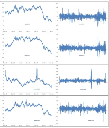
4 Figure 1 provides graphs of the evolution of energy spot price and returns series, respectively, over the sample period.

Energy price fluctuations are not the same in terms of their sizes and duration. This indicates that a dynamic nonlinear structure may exist in the data suggesting the use of nonlinear models, which are able to capture these irregularities.

Price do not exhibit a global trend in the period. Despite many changes, the price has always shown a tendency towards its mean.

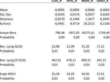
5 Table. 1: Descriptive Statistics

COIL_R HOIL_R NGAS_R GASO_R

Mean -0,0005 -0,0005 -0,0006 -0,0003 Std. Dev. 0,0195 0,0176 0,0357 0,0204 Skewness -0,0579 -0,1494 1,1877 -0,2945 Kurtosis 6,4941 8,4719 29,2512 8,1328

Jarque-Bera 796,48 1957,05 45275,61 1739,49 Probability 0,00 0,00 0,00 0,00

Box- Ljung Q(10) 22,08 21,09 31,20 17,21 Probability 0,01 0,01 0,02 0,02

Box- Ljung Q^2(10) 467,01 478,11 899,31 291,31 Probability 0,01 0,02 0,03 0,03

Engle ARCH 25,18 24,29 34,30 27,41 Probability 0,01 0,01 0,02 0,02

As seen in the table 1, the return series of energy commodity prices have standard deviation of 0.02 on average in the sample period suggesting that it has been highly volatile.

The normality test indicated strong deviation from the skewness and kurtosis from a normal distribution (skewness=0 and kurtosis=3) for all the spot prices. The Jacque-Bera statistics also rejected the hypothesis of normal distribution but has wide tails at the 1% significance level.

Based on the Ljung-Box statistics (10 lags), the null hypothesis of “No serial correlation” is rejected. Similarly, McLeod-Lee statistics reject the null hypothesis of “No serial correlation in squared series” and confirm Heteroskedasticity in return series suggesting that there exists some sort of nonlinear relationship in the squared series. This conclusion is also approved by Engle’s ARCH test as well.

a. Unit Root

According to unit root tests of ADF and PP, the return series is stationary but KPSS and ERS tests unit root test show the series are nonstationary. Thus, such conditions might have been caused by the long memory feature in this series. For this reason, tests for checking the existence of this feature will be focused upon in the next part.

Table. 2: Unit Root Tests

Tests Coil - t stat. Hoil - t stat. Ngas - t stat. Gaso - t stat. t - Critical Result

ADF -41,8669 -42,2717 -35,9824 -41,8235 -1,9416 Stationary PP -41,8660 -42,2632 -35,9795 -41,8156 -1,9416 Stationary KPSS 0,0378 0,0482 0,0444 0,0232 0,1000 Non-Stationary ERS 2,1159 2,3148 1,8892 2,1112 0,4630 Non-Stationary

b. Variance Ratio

6 The random walk hypothesis requires that the variance ratio for all the chosen aggregation intervals, q, be equal to one. If variance ratio is less than one than the series is said to be mean reverting and if variance ratio is greater than one than the series is said to be persistent.

As shown in Table 3, the martingale hypothesis –in the return series- is strongly rejected. So, it can be concluded that the generating process of the data is not random walk.

Table. 3: Variance Ratio Tests

Prob. Stat. Variance Ratio Coil 1.5E-31 -11.69 0.46

Ngas 4.9E-04 -3.49 0.67 Hoil 7.8E-19 -8.86 0.47 Gaso 1.4E-14 -7.69 0.49 3. Long Memory

Long memory property is a sign of strong correlation between far-distance observations in a given time series. Hurst (1951), first, noticed that some time series have this property. However, in mid 1980s, after suggestion of critical concepts like unit root and cointegration, econometricians realized some other types of nonstationarity and partial stationarities which are frequently found in economic and financial time series (Granger and Joyeux, 1980).

Long memory (or long-term dependence) is a special form of non-linear dynamics where a time series has non-linear dependence in its first and second moments and between distant observations, and a predictable component that increases its forecast ability (Thupayagale, 2010). It also means that a time series displays slow decay in its autocorrelation functions (Belkhouja and

Boutahary, 2011). Consequently, “the presence of long memory implies that energy prices (actually returns) tend to be highly volatile, with price changes that often partially cancel out, although the original shock takes a long time to work through the system” (Arouri et al, 2011). The existence of long memory also invalidates the weak-form efficiency of the energy markets because the energy price returns can be predictable (Elder and Serletis, 2008).

Generally, econometricians, used first-order differencing in their empirical analyses due to its ease of use (in order to avoid the problems of spurious regression in non-stationary data and the difficulty of fractional differencing). Undoubtedly, this replacement (of first-order differencing with fractional differencing) leads to over -or under- differencing and consequently loss of some of the information in the time series (Huang, 2010). On the other hand, considering the fact that majority of the financial and economic time series are non-stationary and of the Differencing Stationary Process (DSP1) kind, in order to eliminate the problems related to over differencing and to obtain stationary data and get rid of the problems related to spurious regression, we can use Fractional Integration.

Diagnosing the long memory process is the most important step. Auto Correlation Functions (ACF) as a graphical test and spectral density test or Geweke and Porter-Hudak (GPH) test as the frequently used numeric tests are two main groups of tests that diagnose the long memory feature. In addition to these test, we also performed Hurst exponent and unit root tests.

a. ACF

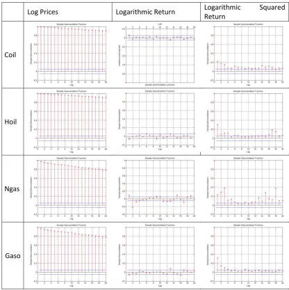
7 represented in the squared returns of the daily energy prices show a typical feature of a long memory volatility property, which is very slow decays at the hyperbolic rate. This finding is in line with the findings of Martens and Zein (2004) and Brunetti and Gilbert (2000) who studied the volatility process of the crude oil futures data.

Log Prices Logarithmic Return Logarithmic Squared Return

Coil

Hoil

Ngas

Gaso

Fig. 2: Auto Correlation Functions

b. GPH Test

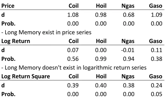
8 Table. 4: GPH Test

Price Coil Hoil Ngas Gaso d 1.08 0.98 0.68 1.09

Prob. 0.00 0.00 0.00 0.00 - Long Memory exist in price series

Log Return Coil Hoil Ngas Gaso d 0.07 0.00 -0.01 0.11

Prob. 0.56 0.99 0.94 0.38 - Long Memory doesn't exist in logarithmic return series

Log Return Square Coil Hoil Ngas Gaso d 0.39 0.40 0.38 0.24

Prob. 0.00 0.00 0.00 0.05 - Long Memory exist in logarithmic squared return series

The results are in line with the ACF outputs.

c. Hurst Exponent

As is well known, systems with different Hurst exponents exhibit different dynamical behaviors:

when 0 ≤ H(τ) < 0.5 the system has antipersistence features; when H(τ) =0.5 the time series is

uncorrelated and indicates a Gaussian or gamma white-noise process. Stochastic processes with

H(τ)=0.5 are also referred to as fractional Brownian motions. The price behaviors exhibit so-called

random walks, while the system’s memory is a Markov chain. When 0.5 < H(τ) ≤ 1 the systems under

study are persistent and characterized by long-term memory that affects all time scales. The time series is initially value-dependent and has chaotic characteristics, thus it is hard to predict future trends. The system has long-term memory of historical information.

Table. 5: Hurst Exponent

Series Coil Hoil Ngas Gaso

Daily Price 0.85 0.86 0.82 0.85

Daily Log. Return 0.53 0.52 0.53 0.52

Daily Squared Log. Return 0.64 0.63 0.62 0.61

Monthly Log. Return 0.76 0.76 0.76 0.77

We observed that there exists 0.5 < H(Τ) ≤ 1 for all price series. That is, the energy price systems

are persistent and autocorrelated and exhibit long-term memory features.

The behaviors of daily returns exhibit distinct persistence and inherent long-term memory. Although the dynamic behaviors of daily returns of energy commodities are close to a Brownian motion, a long term memory mechanism emerges in the two systems as time scales are increased i.e. monthly. The Hurst exponents of daily returns of energy commodities are approximately 0.5, which implies the existence of noise in the systems. However, when time scales increased Hurst exponents of greater than 0.7, which implies that much less noise affects the system dynamics in long-term transaction behaviors. The Hurst exponents of daily squared returns of energy commodities are greater than 0.5, which implies the existence of long-memory in the volatility as well.

9 4. Non-Linearity

a. BDS Test

This test was developed by Brock, Dechert and Scheinkman (1987). The main concept behind the BDS test is the correlation integral, which is a measure of the frequency with which temporal patterns are repeated in the data.

The BDS test is designed to evaluate hidden patterns of systematic forecastable nonstationary in time series. The test constructed to have high power against deterministic chaos, but it was discovered that it could be used to test other forms of nonlinearities as well.

BDS test makes it possible to distinguish between a nonlinear and a chaotic process. The results of BDS test are presented in Table 6.

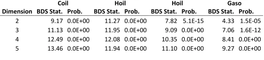
It is evident from the results of the BDS test that the data strongly reject the null hypothesis of iid for all energy prices as the BDS statistic “w” was significant for all embedding dimensions tested. Also, it appears that the evidence of non-linearity was stronger for larger embedding dimensions, as the BDS statistic “w” increased with larger embedding dimensions.

The rejection of the BDS test in energy commodities suggests that the market contains nonlinear dynamics. This is consistent with the observations that energy commodity markets are subject to frequent shocks constantly and major extreme events are prevalent in these markets.

Table. 6: BDS Test

Coil Hoil Hoil Gaso

Dimension BDS Stat. Prob. BDS Stat. Prob. BDS Stat. Prob. BDS Stat. Prob.

2 9.17 0.0E+00 11.27 0.0E+00 7.82 5.1E-15 4.33 1.5E-05 3 11.13 0.0E+00 11.95 0.0E+00 9.09 0.0E+00 7.06 1.6E-12 4 12.49 0.0E+00 12.08 0.0E+00 10.35 0.0E+00 8.41 0.0E+00 5 13.46 0.0E+00 11.94 0.0E+00 11.10 0.0E+00 9.27 0.0E+00 b. Barnett and Wolff Test

BDS test were based on the correlation integral. To acquire more confidence in our results at this point, another test proposed by Barnett and Wolff (2005) is applied, based on high order spectral analysis, namely the third order moment. We set the test parameters in this analysis as recommended by Barnett and Wolff (2005): the embedding dimension we use is 5, the number of bootstrap replications is 1000, and the test significance level is 5%.

The results in Table 7 rejects the null hypothesis of linearity, confirm that the generating forces of the energy spot prices and returns are non-linear.

Table. 7: Barnett and Wolff Test

Price Return

Coil 0.026 0.000 Ngas 0.130 0.000 Hoil 0.036 0.000 Gaso 0.038 0.000 5. Detecting Chaos

10 group of tests available within a nonlinear framework. The tests applied are Lyapunov exponent, correlation dimension and short-term forecast tests.

The BDS tests for iid versus a general nonlinearity in the series. The BDS test by alone does not provide clear evidence for the presence of chaos, even when the null of iid or linearity has been rejected. The correlation dimension is a non-statistical test, which uses integral correlation to test for chaos. The Lyapunov exponent test, however, can be considered as a more direct test for chaos, since it is based on one of the main characteristics of the chaotic series, namely, the extreme sensitivity to the initial condition.

a. Maximal Lyapunov Exponent

Lyapunov exponents (LE) is a quantitative measure of the sensitivity of a time series to the changes in the initial condition. It measures the rate of convergence (divergence) of two initially close points along their trajectory over time. In Lyapunov method, this rate is measured by an exponential function. The value of these exponents can be used to investigate the Local Stability of linear or nonlinear systems. In this test, positive values of exponents indicate exponential divergence of the series, high sensitivity to initial conditions and therefore, chaotic process. On the other hand, negative values of exponents indicate exponential convergence. Finally, when Lyapunov exponents are zero, one may argue that there is no converging or diverging trajectory in the data; i.e. the series follows a fixed process.

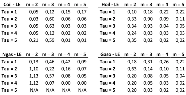
In this study we applied 3 different algorithms to calculate LE’s. i) Rosenstein:

In the method by Rosenstein et al. for each m-dimensional vector ξ in the reconstructed phase space its nearest neighbour ξ* is determined. Rosenstein et al. calculate C(k) ≤ log |f k (ξ)−f k (ξ* )| >

where the angles denote averaging over all ξ = ξ1, ξ2, . . . The function C(k) shows roughly three different regimes. An initial regime of flat increase, a subsequent interval with exponential behaviour, and finally a plateau (because the separation cannot go beyond the extension of the attractor). The maximal Lyapunov exponent is determined by the slope of C(k) in the usually quite short range of exponential behaviour. Positive values of Rosenstein LE’s are referring to the chaotic behaviour of energy prices.

Table. 8: Rosenstein Lyapunov Exponents

Coil - LE m = 2 m = 3 m = 4 m = 5 Hoil - LE m = 2 m = 3 m = 4 m = 5 Tau = 1 0,05 0,12 0,15 0,17 Tau = 1 0,10 0,18 0,22 0,22

Tau = 2 0,03 0,60 0,06 0,06 Tau = 2 0,33 0,90 0,09 0,11

Tau = 3 0,05 0,63 0,03 0,03 Tau = 3 0,34 0,93 0,04 0,05

Tau = 4 0,05 0,12 0,02 0,02 Tau = 4 0,24 0,03 0,03 0,03

Tau = 5 0,21 0,59 0,01 0,01 Tau = 5 0,35 0,02 0,02 0,02

Ngas - LE m = 2 m = 3 m = 4 m = 5 Gaso - LE m = 2 m = 3 m = 4 m = 5 Tau = 1 0,13 0,46 0,42 0,09 Tau = 1 0,18 0,31 0,26 0,22

Tau = 2 1,10 0,22 0,16 0,07 Tau = 2 0,63 0,14 0,10 0,11

Tau = 3 1,13 0,57 0,08 0,05 Tau = 3 0,20 0,08 0,05 0,04

Tau = 4 1,12 0,07 0,00 0,00 Tau = 4 0,20 0,05 0,03 0,02

11 ii) Taylor expansion (Discrete Volterra expansion):

We use a Volterra expansion model to approximate the Jacobian matrix to estimate the LE. Table 9 shows the estimation of the largest Lyapunov exponents for each of the embedding dimensions included in this analysis. As it’s seen, the largest λ was positive for all embedding dimension we tested. The direct interpretation of the Lyapunov Exponent resultsis that the energy commodity spot return series is non-linear deterministic of low dimensions dynamics, i.e., chaos is governing energy commodity returns.

However, to avoid misleading conclusions, the effect of the noise in the data on the LE results can

not be ignored, and can explain the positive values of λ, as Abhyanker, Copeland and Wong (1997)

pointed out.

That’s why we applied chaos testing study in order to conclude that the series are chaotic or not?

Table. 9: Taylor Expansion Lyapunov Exponent

LE m = 2 m = 3 m = 4 m = 5

Coil 0,09 0,19 0,20 0,20 Hoil 0,10 0,23 0,24 0,25 Ngas 0,07 0,16 0,17 0,18 Gaso 0,08 0,17 0,17 0,17

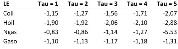
iii) Minimum RMSE neural network

After estimation of network weights and finding network with minimum BIC, derivatives are calculated. Sum of logarithm of QR decomposition on Jacobian matrix for observations gives spectrum of Lyapunov Exponents.

Table. 10:

LE Tau = 1 Tau = 2 Tau = 3 Tau = 4 Tau = 5

Coil -1,15 -1,27 -1,56 -1,71 -2,07 Hoil -1,90 -1,92 -2,06 -2,10 -2,88 Ngas -0,83 -0,86 -1,14 -1,27 -5,53 Gaso -1,10 -1,13 -1,17 -1,18 -1,31

Altough the LE’s found in Rosenstein and Volterra expansion models are positive, LE’s calculated

by minimum RMS neural network model are negative.

Based on these results, we could have concluded that chaotic behavior prevails. This might have been the artifact of the embedding method as it has been expounded in Dechert and Gencay (2000). This is to say that the largest Lyapunov exponent may not be preserved under Takens' embedding theorem.

b. Chaos Testing by Lyapunov Exponent

Chaotic dynamics are closely related in appearance to stochastic dynamics, and the BDS test cannot separate them. Hence, we need a practical test to detect chaos even when the data are noisy.

12 It tests the positivity of the dominant (or largest) Lyapunov exponent λ at a specified confidence level. The test hypothesis H are: null hypothesis H0 : λ > 0, which indicates the presence of chaos; and alternative hypothesis H1 : λ < 0, which indicates the absence of chaos.

Table. 11: Chaos Testing

LE Prob. Chaotic Coil -0,39 0,00 No

Hoil -0,36 0,00 No

Ngas -0,38 0,00 No

Gaso -0,42 0,00 No

Results show that energy commodities doesn’t prevail the chaotic behaviour.

c. Correlation Dimension

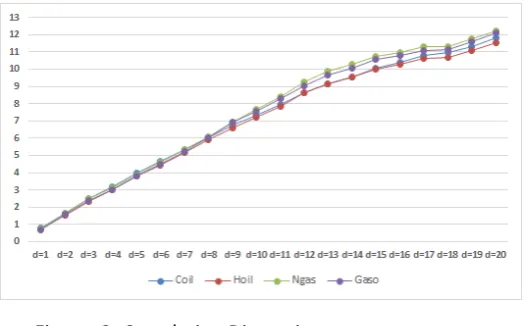
To quantify the degree of complexity of the system that has generated the energy price series, we calculate estimates of the correlation dimension (cd) over the range of embedding dimensions m= 1,

2, …, 20.

If the data are purely stochastic, the correlation dimension will equal m for all m. If the data are

deterministic, the slope estimates will “saturate” or stabilize at some m, not rising any more as m is

further increased. This saturation value of the slope is the correlation dimension estimate for the unobserved underlying process that generated the data.

In this study we applied the Grassberger and Procaccia’s (GP) algorithm to calculate the correlation dimension. However, in interpreting the evidence it should be kept in mind that the GP algorithm may produce estimates with substantial upward bias for attractors and with downward bias for random noise (see (Ramsey and Yuan, 1990; Ramsey et al., 1990)).

Correlation dimension estimates are reported in Figure 2 .The results suggest that the correlation dimension estimates generally increase with embedding dimension but they are below the theoretical values for a completely random process. However, the levels of dimension estimates do not reach a plateau suggesting absence of saturation even though their rate of change with respect to embedding dimension is less than one. Based on this evidence, there is lack of support for a strange attractor in the energy price series. Even if a strange attractor exists, it is not of low dimensionality. Moreover, a correlation dimension greater than about five implies essentially random data.

Figure. 2: Correlation Dimension

13 for chaos in a noisy data may be misleading. Second, as Scheinkman and Lebaron (1989) point out, while an increase in m would not affect the estimate of cd after a certain point for infinite series, it would for finite data. This is particularly important in economic and financial series where the number of observations is very limited compared with empirical sciences.

While the correlation dimension measure is therefore potentially very useful in testing chaos, the sampling properties of the correlation dimension are unknown. As Barnett et al. (1997, p. 306) put it

“if the only source of stochasticity is observational noise in the data, and if that noise is slight, then it

is possible to filter the noise out of the data and use the correlation dimension test deterministically. If the correlation dimension is very large as in the case of high-dimensional chaos, it will be very difficult to estimate it without an enormous amount of data. In this regard, Ruelle (1990) argues that a chaotic series can only be distinguished if it has a correlation dimension well below 2log10 N, where N is the

size of the data set, suggesting that with economic time series the correlation dimension can only distinguish low-dimensional chaos from high-dimensional stochastic processes -see also Grassberger and Procaccia (1983) for more details.

Therefore, the test results based on cd in finite data cannot be conclusive.

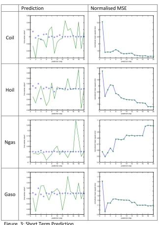
d. Short-Term Prediction

If we have a chaotic time series, we should expect to see predictor error starting out small for a small prediction interval and increasing as the prediction interval increases. No such relationship between predictor error and prediction interval will exist for a randomly-generated time series because the predictor error will always be large.

For a chaotic system and for a given short prediction interval, we should also see predictor errors decrease to a value near zero as d is increased to the correct minimal embedding dimension dE, then increase as d is increased beyond dE . This will not occur for a randomly-generated time series, because the predictor error will be large no matter what embedding dimension is used (Casdagli, 1989).

Prediction is called the "inverse problem" in dynamical systems. That is, given a sequence of iterates from a time series, we want to construct a nonlinear map that gives rise to them. Such a map would be a candidate for a predictive model. The consideration of a nonlinear map is essential, since linear maps do not produce chaotic time series.

Several methods exist for predicting time series. The primary references for our study are Casdagli (1989) and Casdagli et. al. (1992). The methods fall into the categories of global function representation and local function approximation. These functions can be one of the followings: Polynomials, Rational Functions, Wavelets, Neural nets, and Radial basis functions.

In this paper, we demonstrate the method of local fitting, using the ideas contained in Farmer/Sidorowich (1987) and Casdagli et. al. (1992) as our guide.

We use the normalized mean-square-error (E) as a measure of how accurate our predictions are. In order to test our predictions we will need to treat part of the data we have as the training data set (the part we assume we know) and the other part as the test data set, against which we plan to test our predictions.

14 Different choices of k (number of nearest neighbors), N (number of data points in the training data

set), τ (delay), and the multi-step prediction code allows for different choices of T (prediction interval) is used for the prediction study and the following one ise presented as an example.

Number of nearest neighbors; 5, number of data points in the training data set 1.464, delay; 1, prediction interval; 100, embedding dimension; three.

Of the delay parameters τ used, the value of one seemed to result in the most accurate predictions.

Prediction and normalised errors results for energy commodities are as follows: Prediction Normalised MSE

Coil

Hoil

Ngas

Gaso

Figure. 3: Short Term Prediction

E > 1 indicates worse performance of prediction means that the series can not be low-dimensional chaotic but stochastic.

Please note that, since the series is not chaotic, results don’t change for the higher embedding

dimensions., that’s why 3 is set for all predictions.

0 2 4 6 8 10 12 14 16 18 20

-0.06 -0.04 -0.02 0 0.02 0.04 0.06 prediction step ti m e s e ri e s v a lu e 1

0 2 4 6 8 10 12 14 16 18 20

1 1.5 2 2.5 3 3.5 4 prediction step n o rm a liz e d m e a n s q u a re e rr o r

0 2 4 6 8 10 12 14 16 18 20

-0.08 -0.06 -0.04 -0.02 0 0.02 0.04 0.06 0.08 prediction step ti m e s e ri e s v a lu e 1

0 2 4 6 8 10 12 14 16 18 20

1 1.5 2 2.5 3 3.5 4 4.5 prediction step n o rm a liz e d m e a n s q u a re e rr o r

0 2 4 6 8 10 12 14 16 18 20

-0.1 -0.05 0 0.05 0.1 0.15 0.2 0.25 0.3 prediction step ti m e s e ri e s v a lu e 1

0 2 4 6 8 10 12 14 16 18 20

0.4 0.5 0.6 0.7 0.8 0.9 1 1.1 prediction step n o rm a liz e d m e a n s q u a re e rr o r

0 2 4 6 8 10 12 14 16 18 20

-0.08 -0.06 -0.04 -0.02 0 0.02 0.04 0.06 0.08 prediction step ti m e s e ri e s v a lu e 1

0 2 4 6 8 10 12 14 16 18 20

15 6. Conclusion

The limitations and inadequacies of the traditional linear stochastic framework with respect to explaining the dynamics of the behaviour of energy commodity markets has led the recent research to new nonlinear approaches. Among them, chaotic models have attracted increasing attention since they have been shown to exhibit interesting theoretical and empirical features that could help to gain a better insight of the underlying of energy commodity markets mechanisms. However, in order to answer the question of whether low-dimensional chaos may offer a useful way to model the market phenomena, the more fundamental issue of determining whether chaotic behaviour can indeed be observed in energy commodity time series has to be addressed first.

This research starts with a statistical analysis where both series are found to exhibit serial autocorrelation and deviations from normality with fat tails in their distributions.

The empirical analyses presented in this paper have given strong and unambigious support to the existence of nonlinearities in the examined time series.

This result was compatible with a chaotic explanation so we proceeded further with the long-memory tests. Tests reveal long-term long-memory and fractal structure of the series analysed, even in the presence of noise.

To shed more lights on the underlying data generating process of the energy commodity prices, we carried out various tests for deterministic chaos. The tests included correlation dimension, and Lyapunov Exponent.

The energy price series exhibited non-saturating correlation dimension, which in addition was not significantly different than the dimension of random series having the same distributional characteristics.

The largest Lyapunov exponent estimation was found to verify the possibility of a chaotic component in the energy commodity series. However, we show that this method, at least with the algorithm that we have employed (the most commonly used in the literature), is not by its own a reliable method to detect chaoticity since it is unable to distinguish between alternative specifications such as chaotic, Gaussian random, and fractal random sequences.

In a final step, the existence of a chaotic component in the energy commodity series was further investigated through nonlinear forecasting techniques based on phase space reconstruction. The results from these applications were compatible with our previous findings; the fitting precision is very low and the model has the very poor forecast effect which results in not showing chaotic behaviour.

16 7. Literature

Abarbanel H.D.I., Brown R. and M. B. Kennel, 1991, Variations of Lyapunov exponents on a strange attractor, Journal of Nonlinear Science 1, 175-199.

Abarbanel H.D.I., Brown R. and M. B. Kennel, 1992, Local Lyapunov exponents computed from observed data, Journal of Nonlinear Science 2, 343-365.

Abarbanel, H. D. I., 1996, Analysis of Observed Chaotic Data. Springer. New York.

Adrangi, B., Chatrath, C., 2001, Chaos in oil prices? Evidence from futures market Energy Economics 23 405-425

Bask, M. and Gençay, R., 1998, Testing chaotic dynamics via Lyapunov exponents, Physica D 114, 1-2.

Bask, M., 1998, Deterministic chaos in exchange rates?, Umeå Economic Studies No 465c, Department

of Economics, Umea University , Sweden

BenSaida, A., 2014, Noisy chaos in intraday financial data: Evidence from the American index. Appl Math Compu., 226, 258–65

BenSaida, A., 2015, A practical test for noisy chaotic dynamics, ScienceDirect, SoftwareX 3–4, 1–5

Brock, W., Dechert, W., Scheinkman, J. and B. LeBaron, 1996, A test for independence based on the correlation dimension, Econometric Reviews 15, 197-235.

Chatrath, A., Adrangi, B., Dhanda, K., 2002, Are commodity prices chaotic? Agricultural economics 27 123-137

Dechert W. and Gençay, R.,1992, Lyapunov exponents as a nonparametric diagnostic for stability analysis, Journal of Applied Econometrics 7, S41-S60.

Dechert W. and R. Gençay, 2000, Is the largest Lyapunov exponent preverved in embedded dynamics?,

Physics Letters A 276, 59-64.

Eckmann J. P., Kamphorst S. O., D. Ruelle, and S. Ciliberto, 1986, Lyapunov exponents from time series, Phys. Rev. A, 34, no. 6, pp. 4971-4979

Eckmann, J. P. and D. Ruelle, 1985, Ergodic theory of chaos and strange attractors. Reviews of Modern Physics, 57, 617-650.

Gençay, R. and W. Dechert, 1992 , An algorithm for the n Lyapunov exponents of an n-dimensional unknown dynamical system, Physica D 59, 142-157.

Gençay, R. and W. Dechert, 1996, The identification of spurious Lyapunov exponents in Jacobian

algorithms, Studies in Nonlinear Dynamics and Econometrics 1, 145-154.

17 Grassberger, P. and I. Procaccia, 1983, Characterization of Strange Attractors, Physical Review Letters 50, 346-394.

Gunay S., 2015, Chaotic Structure of the BRIC Countries and Turkey’s Stock Market. International Journal of Economics and Financial Issues, 5(2), 515-522.

Kantz H. and Schreiber T., 2004, Nonlinear time series analysis. Cambridge University Press, 2nd edition.

Panas, E., Ninni, V, 2000, Are oil markets chaotic? A nonlinear dynamic analysis Energy Economics 22 549-568

Rosenstein, M., Collins, J.J. and De Luca, C.,1993, A practical method for calculating largest Lyapunov exponents from small data sets, Physica D 65, 117-134.

Schuster H. G., 1995, Deterministic Chaos: an introduction’, VCH Verlasgesellschaft, Germany.

The MathWorks, Inc., 2015, MATLABR—The Language of TechnicalComputing, Natick, Massachusetts, URL http://www.mathworks.com/products/matlab.