Munich Personal RePEc Archive
The asymmetric housing wealth effect on
childbirth
Iwata, Shinichiro and Naoi, Michio
1 July 2015
Online at
https://mpra.ub.uni-muenchen.de/65360/
The asymmetric housing wealth e¤ect on childbirth
Shinichiro Iwata
Faculty of Economics, University of Toyama
Michio Naoi
Faculty of Economics, Keio University
July 1, 2015
Abstract
The literature has shown that an increase in housing wealth, driven by unexpected shocks to house prices, exerts a positive e¤ect on the birthrates of homeowners. According to canonical models, a decrease in housing wealth has a symmetric negative impact on the fertility behavior of households. That is, housing gains and losses of the same size should have identical quantitative e¤ects on fertility. In comparison, prospect theory suggests that people care more about housing losses than equivalent gains, leading to an asymmetric e¤ect of housing wealth on the fertility decision. In our model, we weight the utility from childbirth by the utility from the price of housing, where the reference level is the house price in previous years. The theoretical model suggests that the probability of childbirth is kinked at a reference level of housing wealth and the wealth e¤ects are discontinuously larger below this kink than above it. We test this theoretical prediction using longitudinal data on Japanese households. Consistent with this theoretical prediction, our empirical results show that the fertility responses of homeowners, as measured by the birth hazard rate, are substantially larger when housing wealth is below its reference level than when it is above its reference level.
1
Introduction
Owner-occupied housing is the most signi…cant form of wealth holding for both young and
middle-aged households in Japan.1 Using microdata from the Nikkei Radar (1987–99), which
covers households in the Tokyo metropolitan area, Iwaisako (2009) demonstrated that housing
wealth accounts for approximately 90 percent of the total wealth of homeowners in their 20s, and
approximately 80 percent of those in their 30s and 40s. Nonetheless, housing wealth ‡uctuates
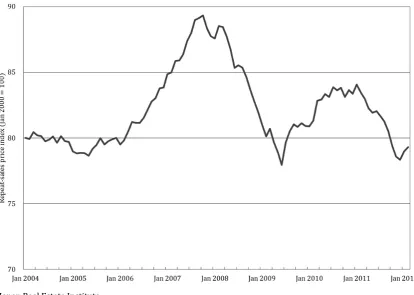
markedly because of variations in house prices. Figure 1 depicts the Japan Real Estate Institute
(JREI) Home Price Index, which is based on the price changes for repeat sales of second-hand
condominium properties in the Tokyo metropolitan area.2 As shown, after a signi…cant decline
in the early 2000s, house values reversed the downward trend in 2005 and reached a peak
in October 2007. Housing prices then fell sharply in 2008 and 2009, possibly because of the
subprime mortgage crisis. While house values recovered somewhat in 2010, they fell again in
2011.
A voluminous literature has investigated how house price ‡uctuations a¤ect household
con-sumption decisions. In a pioneering study, Case et al. (2005) argued that the housing wealth
e¤ect on consumption has become increasingly important, as institutional innovations have made
it simpler to extract cash from housing equity. They hypothesized, and were duly supported
by empirical results, that exogenous changes in house prices are associated with changes in
the available housing equity, thereby changing consumption. More recently, Lovenheim and
Mumford (2013) and Dettling and Kearney (2014) have applied the housing wealth e¤ect to
the childbearing choices of households.Using the same logic, they hypothesized that changes in
home value imply changes in wealth for current homeowners, and that these changes could
con-sequently a¤ect child bearing decisions.Their empirical results indeed suggested that children
are normal goods and that an increase in house prices tended to encourage child bearing among
homeowners.
In general, household fertility decisions are an important issue in Japan because the total
1According to the 2008 Housing and Land Survey, the homeownership rate of Japanese aged 25–29 years was
11.5 percent, while that of those in their 30s and 40s was 38.8 percent and 62.2 percent, respectively.
fertility rate was at its lowest level of just 1.26 in 2005. Since then, the total fertility rate has
risen slightly, down 0.01 percentage points from the previous year to 1.42 in 2014. A recent
article has sounded the alarm that the total fertility rate is headed for a long-term decline
as second-generation baby boomers, born between 1971 and 1974, pass their peak childbearing
years.3 Examining the purported link between changes in housing wealth and household fertility
decisions could then inform this issue. However, unlike Lovenheim and Mumford (2013) and
Dettling and Kearney (2014), we shed light on an asymmetry in the response to unanticipated
housing wealth gains and losses. If we consider the housing wealth e¤ect on childbirth only
through the budget constraint, as in Lovenheim and Mumford (2013) and Dettling and Kearney
(2014), we cannot derive this asymmetric e¤ect. We thus examine the impact through a di¤erent
channel by applying prospect theory as developed by Kahneman and Tversky (1979). This
theory suggests that households care more about wealth losses than equivalent gains through
the value function. In fact, the empirical results in Genesove and Mayer (2001) demonstrated
that homeowners with a potential loss behave di¤erently when compared with those with an
equivalent-sized prospective gain. In our model, the utility from childbirth is weighted by the
utility from the change in house prices, where the reference level is based on the house price in
previous years. The theoretical model then suggests that the probability of childbirth is kinked
at a reference level of housing wealth and that the wealth e¤ects are then discontinuously larger
below the kink than above it.
We test this theoretical prediction using longitudinal data on Japanese households collected
by Keio University. The Keio Household Panel Survey (KHPS) is a nationally representative,
large-scale survey that commenced in 2004 with an initial sample of approximately 4,000
house-holds. We use eight waves of the KHPS from 2004 to 2011. As shown in Figure 1, this period
appears to be ideal for examining the supposed asymmetric housing wealth e¤ect because the
housing market has experienced both price increases and price decreases. These variations in
housing wealth are captured by the relative change in reported home values, where
self-reported home values in previous years serves as the reference level. We measure childbearing
3Bracing for demographic change: Japan’s fertility rate headed for long-term decline. Nikkei Asian
choices using the birth hazard rate and estimate proportional hazard models to understand the
relationship between changes in housing wealth and family formation behavior. Our empirical
results suggest that, consistent with our theoretical prediction, the fertility responses of
home-owners are substantially larger when housing wealth is below its reference level than above.
Using our empirical results, we then simulate the e¤ect of a one million yen change in house
values on the hazard rate. Our estimates indicate that a one million yen decrease in house values
decreases the hazard rate of childbirth by approximately 10.9 percent, whereas a one million
yen increase in house values leads to an increase in the childbirth hazard rate by a mere 1.0
percent. This suggests that encouraging childbirth through boosting housing markets will entail
a di¤erent magnitude of impact, depending on housing price gains and losses.
2
Literature review
2.1 The e¤ect of housing wealth on consumption
Case et al. (2005) used two panels of cross-sectional time series data: one for developed countries
measuring aggregate consumption and aggregate housing wealth; and the other for US states
measuring aggregate retail sales as a proxy variable for aggregate consumption and the aggregate
value of owner-occupied housing. Although the impact was rather small, the empirical results
demonstrated that changes in housing prices have a signi…cantly positive impact on household
consumption in the US and other developed countries. Subsequently, Case et al. (2013) extended
the panel of US states used in their earlier study, by incorporating substantial periods of declines
in housing prices. As a result, they identi…ed the statistically signi…cant and rather large e¤ect
of housing wealth on consumption spending. Campbell and Cocco (2007) used household-level
data from the UK family expenditure survey to estimate the response of consumption to house
prices. Their benchmark model suggested that the elasticity of consumption to house prices is
indeed elastic. Paiella (2009) provides a detailed review of this literature.
Elsewhere, Genesove and Mayer (2001) applied the prospect theory developed by Kahneman
and Tversky (1979) and Tversky and Kahneman (1991) to the housing market. After introducing
houses, they hypothesized that a seller with a potential loss would be expected to set a higher
price and face a lower hazard rate of sale than a seller with an equivalent-sized prospective gain.
Indeed, their empirical results, using data from the Boston condominium market, indicated
that sellers behave as predicted by the prospect theory. Motivated by this analysis, Case et
al. (2013) hypothesized that the painful regrets associated with decreases in home values exert
stronger psychological consequences than does the pleasant elation associated with increases in
home values, such that homeowners behave asymmetrically as to the gains and losses in housing
wealth. The empirical results suggested that an increase in housing wealth has a positive e¤ect
on household consumption, while a decline in housing wealth has a negative and somewhat larger
e¤ect on consumption, both being consistent with the prospect theory.
Using household-level panel data from the US, Engelhardt (1996) also suggested that
sav-ings display signi…cant asymmetry in response to unanticipated gains and losses from housing.
That is, homeowners experiencing a housing capital gain do not alter savings behavior, while
those experiencing a loss tend to increase savings. Likewise, Disney et al. (2010), using UK
household panel data along with county-level house price data, demonstrated that households
experiencing an unanticipated loss exhibit a larger reaction in savings than those experiencing
an unanticipated gain. However, these di¤erences were found to be not statistically signi…cant.
2.2 The e¤ect of housing wealth on childbirth
Lovenheim and Mumford (2013) and Dettling and Kearney (2014) argued that house price
movements are appropriate for examining how increases in individual income a¤ect fertility
because changes in house prices do not a¤ect the cost of parental time to raise children in the
same way that changes in market wages do. An increase in the market wage implies an increase
in the value of time spent on labor; thus, the substitution e¤ect reduces fertility (Becker 1965).
An increase in housing prices also involves a negative substitution e¤ect on the demand for
children, especially for prospective homeowners who would purchase a house with the addition
of a child, when the association between children and housing is a complement. However, as
discussed, rising home values imply a boost in wealth for current homeowners. Consequently,
Even though homeowners do not intend to resell their housing, they can use the increase in
equity to fund their childbearing goals (the equity extraction e¤ect).
Lovenheim and Mumford (2013) also noted that house price movements are valid because
they can be used to generate exogenous shocks to household wealth, which overcomes the
endo-geneity between wealth accumulation and childbirth decisions. Using US individual-level data
(1985–2007), they estimated linear probability models for families giving birth in a given year
as a function of two- and four-year changes in self-reported home values. The empirical results
demonstrated that a $100,000 increase in an individual’s real housing wealth among homeowners
was associated with a 16.4 percent increase in the probability of having a child. By comparison,
among renters, Metropolitan Statistical Area (MSA)-level housing price growth had no
signi…-cant e¤ect on current fertility. Because the positive e¤ect of home price changes on childbirth
is only observed for homeowners, these tend to capture the hypothesized wealth e¤ect.
Although Lovenheim and Mumford (2013) considered that house price movements are
exoge-nous, potential endogeneity issues remain. For example, households that plan to have children
may purchase homes in good neighborhoods, therefore self-selecting into locations that are more
likely to experience high housing price growth in the future. Such selection mechanisms bias
upwards conventional estimates of the e¤ect of house price growth on fertility. To address this
possibility, Dettling and Kearney (2014) used MSA-level housing supply elasticity as an
in-strumental variable (IV) and estimated IV regression of MSA-level fertility rates on MSA-level
house prices during the 1997–2006 housing boom period. Their IV estimates demonstrated that
short-term (one-year) increases in house prices led to a decline in births in places where the
homeownership rate was relatively low. However, this decline was outweighed by the increase in
births where the homeownership rate was relatively high. That is to say, similarly to Lovenheim
and Mumford (2013), they found fertility rates for homeowners were positively associated with
short-term increases in house prices. In sum, at the mean US home ownership rate in their
sam-ple period, the net e¤ect of a $10,000 increase in house prices produced a 0.8 percent increase in
fertility rates. They also con…rmed the …ndings of previous analysis using aggregate-level data
house prices conditional on MSA …xed e¤ects to control for endogenous sorting into higher- or
lower-priced MSAs.
These estimates appear to predict that a housing market decline may have a symmetric
neg-ative impact on fertility. If true, it may help us to understand whether the severe price declines
in the housing market following the US subprime mortgage crisis is one of the reasons for the
fairly sharp decline in the US birth rate. To examine this hypothesis, Lovenheim and Mumford
(2013) used the 16.8 percent of the subsample that experienced price declines. Although they
found some evidence that the response was not symmetric, they also found that the e¤ect of
falls in home values was not statistically di¤erent from zero. This suggests that fertility
deci-sions are less likely to respond to housing market variation during a period of house price falls.
Lovenheim and Mumford (2013), however, suggested that more work examining the e¤ect of the
housing bust on fertility was needed in the future when data from the period of the housing bust
became available. On the other hand, Dettling and Kearney (2014) used data from the housing
bust period of 1990–96, and conducted a similar exercise. The empirical results from this period
are similar to the housing boom period, supporting a symmetric negative impact.4 They also
con…rmed similar results during the recent housing bust period of 2007–10, even though only
individual-level data were used because MSA-level fertility rates were not available at the time.
In sum, Dettling and Kearney (2014) suggested that fertility responses tend to be symmetric
irrespective of the rise or fall of house prices, whereas Lovenheim and Mumford (2013) suggested
that fertility is more likely to respond when house prices increase than decline. However, both
these results are largely inconsistent with prospect theory, which suggests that households care
more about wealth losses than equivalent gains.
3
The theory of childbirth and housing wealth
Let us de…ne Bt as a parameter indicating the propensity to undergo a birth at time t, which
is endogenously selected by families dwelling in owner-occupied housing. If families do not have
a birth, then Bt = 0, whereas if they do, then Bt = 1. We treat Bt as a continuous variable
4However, they argued that the impact appeared to be symmetric because the sign of the coe¢cients was
that ranges from zero to one, because it allows us to di¤erentiate the objective function, as
shown below. Therefore,Btrepresents the probability of childbirth in our context. Let us de…ne
U(Bt) as the utility from expecting to have a child and C(Bt) as the cost function. Assume
thatU0(B
t)>0,U00(Bt)<0,C0(Bt)>0, and C00(Bt) = 0. The household surplus from having
a child can then be written as U(Bt) C(Bt). To introduce the impact of housing wealth on
utility, assume that the utility function U(Bt) is weighted by a value function that depends
on current housing wealth, Wt. In this analysis, we assume Wt is exogenous for families. The
value function captures that the behavior of family members is a¤ected by the estimated value
of their housing. We de…ne the house price in the prior yearWt 1 as the reference wealth level.
To apply the theory of reference-dependent preferences, the optimal level ofBt is then chosen
by maximizing the following modi…ed surplus functions:
U(Bt) (Wt) C(Bt) if Wt Wt 1; U(Bt) (Wt) C(Bt) if Wt Wt 1;
where (Wt) and (Wt) represent the value functions. The value functions are assumed to
follow diminishing marginal utility over wealth. That is, 0(W
t)>0, 00(Wt)<0, 0(Wt) >0,
and 00(W t)<0.
Assume (A1) (Wt 1) = (Wt 1). This assumption ensures that the value functions take
the same value at the reference point. Assume also that (A2) 0(W
t 1) < 0(Wt 1). This assumption re‡ects that families are loss averse: that is, they are more sensitive to losses than
gains, resulting in a greater marginal utility change for losses (Tversky and Kahneman 1991).
The …rst-order condition for the above problems is:
U0(B
t) (Wt) C0(Bt) if Wt Wt 1; U0(B
t) (Wt) C0(Bt) if W Wt 1:
Let us denoteBt as the optimal level atWt=Wt 1. Di¤erentiating the …rst-order condition
with respect to housing wealth atWt=Wt 1 can be written as:
dBt
dWt Wt=Wt
1 = 8 > > < > > :
U0(B t)
U00(B t)
0(W t 1)
(Wt 1)
>0 if Wt Wt 1;
U0(B t)
U00(B t)
0(W t 1)
(Wt 1)
>0 if W Wt 1:
Because 0(W
t 1)= (Wt 1)< 0(Wt 1)= (Wt 1) by assumptions (A1) and (A2), equation (1) demonstrates that the optimal propensity to have a child is kinked at the reference housing
wealth and that the marginal propensity with respect to an exogenous increase in housing
wealth is discontinuously higher below the kink than above it. This suggests a negative e¤ect
on fertility because the decline in house prices from the reference point is more pronounced than
the positive e¤ect on fertility, as derived from an unexpected rise in house prices.
4
Empirical analysis
4.1 Data and variables
Our empirical analysis draws on the Keio Household Panel Survey (KHPS) to examine the
relationship between housing wealth and the fertility decisions of homeowners. The KHPS,
sponsored by the Japan Society for the Promotion of Science (JSPS), is a nationally
represen-tative, large-scale longitudinal survey of Japanese households that commenced in 2004 with an
initial sample of approximately 4,000 households. In 2007, a random refreshment sample of
approximately 1,400 new respondents addressed panel attrition. In the following analysis, we
use eight waves of the KHPS from 2004 to 2011. The KHPS is particularly suited to
address-ing the research questions in this paper because it contains detailed information on household
demographic events, including childbirth, the tenure mode of housing and housing wealth, and
includes a rich set of family background characteristics.
In the following analysis, a dichotomous variable indicating childbirth represents the event
of interest. This variable takes a value of one if the respondent family had a new baby in the
last 12 months, and zero otherwise. Duration is de…ned as follows: 1) years since marriage for
those without any child; 2) years since last childbirth for those having at least one existing child.
The KHPS also provides information on the value of the home if it is owned.5 Similar
to Lovenheim and Mumford (2013), our housing wealth measure is constructed based on
self-reported information in the survey (“How much do you think the house and lot would sell for
on today’s market?”). One could be skeptical about the use of self-reported house values as
5There are no publicly available data for housing prices in Japan, except the JREI Home Price Indices, which
a proxy for market values. The owner’s valuation can be inaccurate and include a systematic
bias toward optimistic evaluation. In fact, Kiel and Zabel (1999) showed that the average owner
overstates their house value by 5.1%. Using self-reported house values can pose a serious problem
in our application if the measurement errors in an owner’s valuation are correlated with birth
behavior. This can be possible if there are some omitted variables in our model that are also
correlated with self-reported house values. Again, however, Kiel and Zabel (1999) showed that
valuation errors are not correlated with owner’s individual characteristics as well as the house
and neighborhood attributes. Furthermore, because our housing wealth measure is the change
in self-reported values, problems arising from systematic overvaluation can be largely mitigated.
In fact, several previous studies have shown that owners’ valuations result in accurate estimates
of house price indices (Kiel and Zabel 1999; Lovenheim 2011). Overall, we believe that using
self-reported values will represent only a minor problem in our speci…c application. In the following
analysis, we assume that the reference wealth level is de…ned as the status quo, that is, the
self-reported value in the previous year,Wt 1. This is a standard assumption in the literature
where the reference state corresponds to the decision maker’s current endowment (Tversky and
Kahneman 1991; Dettling and Kearney 2013).
In addition to these variables, we gather a number of important economic and demographic
characteristics from the KHPS. These include a dummy variable indicating the number of
exist-ing children prior to the new childbirth in question, the female respondent’s age and its square,
the level of completed education (high school, technical college/vocational school, two-year
col-lege, and four-year college or higher), employment status (not employed, employed part-time,
and employed full-time), and male respondent’s labor earnings.6 We also control for region, city
size, and survey year using dummy variables in each of our estimations. All monetary variables
are converted to 2005 prices using the Consumer Price Index.
The original survey includes 4,005 households in 2004 (wave 1) with 1,419 households added
in 2007, resulting in 5,424 unique households. Of these households, 870 households participated
in the survey only once (i.e., dropped out in the second wave). As we use lagged information
6Women’s employment careers are likely to be interrupted by childbirth and infant care, leading to a typical
(i.e., household and housing characteristics from the previous wave) in our empirical analysis,
we exclude these households, resulting in 4,554 unique households.
As our purpose is to identify the impact of self-reported house values on childbirth, we
re-stricted our sample to homeowners who did not move during the survey period. For mover
house-holds, changes in self-reported house values cannot be interpreted as real house price changes.
Furthermore, house values can increase through additions and/or repairs, even when market
prices are stable. We therefore exclude homeowners that made any additions and/or repairs to
their home from our sample. This reduced our sample further to 3,407 unique households.
The sample was further restricted to households with a married woman of childbearing age,
i.e., a female respondent aged between 20 and 50 years. This reduced the number of unique
households further to 1,250. This reduction is substantial because the KHPS covers both
single-person (unmarried) households and the elderly. Finally, restricting the sample to those where
all necessary information was available further reduced the number of unique households to 932.
Taking each household-year pair as a unit of observation, our estimation is based on a total of
2,893 observations.
Table 1 provides selected descriptive statistics for our variables. The childbirth dummy
has an average value of approximately 0.02, indicating we have a total of 60 births in our
observations during the sample period. One reason for this low value may be that the average
age of female respondents is approximately 41 years, as reported in Table 1, and they already
have approximately two children on average (not shown). The mean self-reported home values
is approximately 23.1 million yen (not shown). On average, home values decreased by about 1.5
million yen during the sample period.
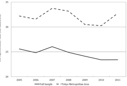
Figure 2 illustrates the average self-reported home values over time. As shown, the average
house values increased from 2006 to 2007. Afterwards, house values steadily declined until 2010
where they remained through to 2011. The average self-reported home values in the Tokyo
metropolitan area also display the same tendency. However, from 2010 to 2011, average
self-reported home values increased in the Tokyo metropolitan area.
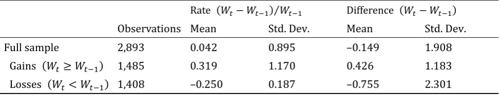
on whether they had experienced housing price gains or losses. For the sake of simplicity, we
categorize these into housing wealth gainers and losers, where the former also includes those
who reported the same house value as the previous year (524 observations).7 Approximately
half of the observations showed price increases. For these, home values increased approximately
4.3 million yen on average. Excluding households that reportedWt =Wt 1, the average price
appreciation was 6.6 million yen. The remaining half of the observations experienced price
declines. For these, home values decreased approximately 7.6 million yen on average. In sum,
our dataset appears to cover well both housing wealth gainers and losers.
4.2 Econometric model
Because our data are in the form of panel data, we analyze decisions on childbirth within the
framework of a duration model. We thus modify the notation of our theoretical model, such
that instead ofBt, we use the birth hazard rateB(t). The birth hazard rate is the probability
that childbirth is realized, given that the birth interval lasts at least until t. Our benchmark
proportional hazard model can be written as:
B(t) =B0(t;Y; M) exp Gd[Wt Wt 1]
Wt Wt 1 Wt 1
+ Ld[Wt<Wt 1]
Wt Wt 1 Wt 1
+ X(t) ;
(2)
whereB0 is an unknown baseline hazard att. In order to control for underlying heterogeneity
in birth behavior, we stratify the baseline hazard by the year of birth(Y)and the year in which
households moved into the current residence(M).8 This allows us to control for cohort e¤ects, as
suggested by Hashimoto and Kondo (2012), and the e¤ects of di¤erent housing market conditions
at the time of home purchase. For the latter, Öst (2012) suggested that institutional factors
in the housing market, such as the housing subsidies and tax bene…ts associated with home
purchase, can potentially a¤ect subsequent birth behavior. X(t) is a set of other explanatory
variables, and is the corresponding parameter vector. d[A] is an indicator function that takes
7However, whether we include these households with the housing gainers does not fundamentally change our
results. See the discussion in Section 4.4.
8In the estimation, we classify female respondents into three groups based on their birth year (born in and
a value of one if the event A is true, and zero otherwise. Therefore, holding all other things
constant, the e¤ect of the annual percentage changes in housing wealth on the birth hazard
rate can be represented by G if Wt Wt 1, and L if Wt < Wt 1. Our theoretical model
predicts that the optimal propensity to have a child is kinked at the reference housing wealth
and that the marginal propensity with respect to an exogenous increase in housing wealth is
discontinuously higher below the kink than above it. This implies that G< L.
4.3 Empirical results
As a preliminary step, we begin by considering a simpler model excluding any asymmetric impact
of housing wealth on fertility decisions. Speci…cally, we estimate the model given by equation
(2) with the restriction that G = L. We estimate the model by applying a standard Cox’s
proportional hazard model for childbirth. Table 3 presents the empirical results. The results
in column [1] show that a short-term increase in house prices is positively associated with the
homeowner’s probability of giving birth in a given year. This result is consistent with previous
…ndings in the literature. However, Lovenheim and Mumford (2013) and Dettling and Kearney
(2014) used data from a housing boom period, while our data include both housing boom and
bust periods. The signi…cantly positive sign indicates that during a housing boom (bust) period,
an increase (decrease) in house prices leads to a positive (negative) wealth e¤ect on the fertility
decisions of homeowners. In addition, we also present regression results using an alternative
speci…cation for the housing wealth measure, i.e., annual changes in the level of self-reported
house values(Wt Wt 1), in column [2] of Table 3. These results also suggest that short-term
increases in house prices are positively associated with the homeowner’s probability of giving
birth.
In terms of the demographic and family background variables, our results are as follows.
Female respondent’s age has a signi…cant nonlinear e¤ect on childbirth. The estimated results
show that the probability of giving birth increases through the female respondent’s 20s, reaching
a maximum at around 30, and then decreasing throughout the respondent’s 30s and 40s. The
number of existing children is signi…cantly and negatively associated with the probability of have
respondents with a four-year college or postgraduate degree tend to have a signi…cantly lower
probability of giving birth. As expected, female employment status is associated with childbirth.
Compared with respondents not working, the probability of giving birth is considerably lower
for those working part or full time (in year t 1), although the estimated coe¢cient is not
signi…cant in the case of the latter.
Given these preliminary results, we now test the asymmetric impact of housing wealth on the
fertility decision. The results are in columns [3] and [4] of Table 3. The null hypothesis of equal
wealth coe¢cients,H0: G= L, is tested against the one-sided alternativeHa: G< L. From
column [3], we …nd that the estimated coe¢cient on short-term increases in housing values is
signi…cantly positive whenWt< Wt 1 (coef. = 2.684). In comparison, the estimated coe¢cient
on short-term increases is still positive but considerably smaller and statistically insigni…cant
when Wt Wt 1 (coef. = 0.227). This is consistent with our theoretical prediction that the
fertility responses of homeowners are substantially larger when their housing wealth is below
its reference level than when housing wealth is above its reference level. As a result, the null
hypothesis of equal wealth coe¢cients,H0: G= L, is strongly rejected. The results in column
[4] using annual changes in the level of house values yield qualitatively similar …ndings.
In order to evaluate the results in column [3] quantitatively, we calculate the predicted e¤ect
of a one million yen change in house prices on the birth hazard rate. Given that the average
house value in our dataset is 23.1 million yen, a one million yen change translates into a relative
house value change of 0.043, which is close to the mean rate of change given in Table 2 (0.042).
Our coe¢cient estimate of L suggests that households facing a one million yen decrease in
their house values were approximately 10.9 percent less likely to have an additional birth in the
following year (1 e 0:043 L = 0:109). Conversely, a one million yen increase in house values
corresponds to a mere 1.0 percent increase in the hazard rate (e 0:043 G = 1:010).
4.4 Robustness checks
The remainder of this section reports the results of additional speci…cations to assess the
robust-ness of our main …ndings. We estimate three alternative models in addition to our benchmark
in the past two years, (Wt Wt 2)=Wt 2, as an alternative wealth measure. This enables us
to examine longer-term e¤ects of housing wealth changes on childbirth. The estimated results
show qualitatively the same pattern as our benchmark results.
As we assume that the reference wealth level coincides with the status quo (Wt 1), any
measurement errors in past house values can bias our results. Measurement error in past house
values presumably poses a particularly serious problem if current housing wealth is not so
dif-ferent from the reference wealth level (i.e., Wt Wt 1). This is because only a small amount
of measurement error in the past house values can change whether a particular household has
housing wealth above (or below) the reference level. Therefore, in column [2] of Table 4, we
exclude households that report the same self-reported house values across adjacent years, i.e.,
Wt = Wt 1. Because 524 households reported exactly the same house values across adjacent
years, this substantially reduces our sample size. The estimated results presented in column
[2], however, are qualitatively similar to our benchmark results. The estimated coe¢cient on
housing losses (coef. = 3.112) is somewhat larger than in our benchmark result, but we continue
to observe an asymmetric wealth e¤ect. We therefore believe that measurement errors do not
pose serious problems in our estimation.
In column [3] of Table 4, we estimate the same model using the sample households that
already had at least one child (i.e., second and subsequent births) in order to examine whether
homeowners’ fertility responses di¤er for …rst and subsequent births (Lovenheim and Mumford
2013). The estimated coe¢cient on housing losses turns out to be larger than in our benchmark
result, consistent with previous …ndings. While fertility responses for …rst births might be
interpreted as changes in the optimal timing of childbirth, those for second and subsequent
births may represent changes in the total number of children. Therefore, our results suggest that
housing wealth a¤ects not only the timing of childbirth but also the total number of children.
In Table 5 we present several alternative models allowing for more ‡exible speci…cations of
housing gains/losses. In column [1], we added a dummy variable indicating whether respondents
experienced housing gains. Our theoretical model assumes that the value function is continuous
variable has a statistically insigni…cant coe¢cient estimate for childbirth. In addition, the
coe¢cient estimates for changes in self-reported house values are quantitatively similar to our
benchmark results in column [3] of Table 3.
In column [2] of Table 5, we adopt a quadratic speci…cation for both housing gains and
losses. This speci…cation is useful for testing whether the asymmetric housing wealth responses
in the benchmark results are driven by potential nonlinearity of the e¤ects of the housing gains
and losses. The estimated results, however, indicate that the quadratic terms for housing gains
and losses are both statistically insigni…cant, implying that the underlying relationship between
housing wealth and fertility may not be (at least quadratically) nonlinear.9
Up to now, we have exclusively focused on existing homeowners to evaluate the e¤ects of
housing wealth on childbirth. As discussed earlier, a rise in house prices will increase the available
resources of homeowners, and may lead to a positive e¤ect on fertility decisions. An increase in
house prices, on the other hand, will have the opposite e¤ect on prospective owners (i.e., renters),
as this will require a larger deposit for future home purchases and reduce the available resources
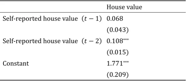
for these households. In order to examine the e¤ects of housing price changes on renters, we
derive year-on-year changes in regional house prices by regressing the homeowner’s self-reported
values on region–city size …xed e¤ects.10 The estimation results for the house value regression
imposing an AR(2) process are in Table 6. We obtains the predicted house value changes for
each region–city size–year combination using these results.
Table 7 provides our estimation results using regional house value changes. The …rst two
columns present the regression results for homeowners. In column [1], although the coe¢cient
estimate is not statistically signi…cant, we can see that changes in regional house values have a
positive e¤ect on childbirth. In addition, allowing for an asymmetric e¤ect, as in column [2] of
Table 7, we can see that changes in regional house values have a signi…cantly positive coe¢cient
9Instead of rate changes in self-reported values, we use absolute change in self-reported values and its square.
Although we were unable to stratify the baseline hazard because of a problem with convergence, a quadratic speci…cation …ts both housing gains and losses well. Even with this quadratic speci…cation, we still …nd that the fertility responses are asymmetric in terms of housing gains and losses. That is, housing losses have a larger impact on fertility than do gains of an equivalent size.
1 0KHPS categorizes a respondent’s location of residence in eight regions (Hokkaido, Tohoku, Kanto, Chubu,
estimate only when regional house values decrease. Overall, the estimated coe¢cients on housing
wealth variables display a qualitatively similar pattern as our benchmark case in columns [1]
and [3] of Table 3, implying that our predicted house value changes well capture any regional
house price variation. The regression results for renter households are in column [3]. As shown,
regional house price changes have a negative, although not statistically signi…cant, impact on
renter fertility decisions (Lovenheim and Mumford 2013).
5
Conclusion
This paper estimated the responses of homeowner childbirth to changes in housing wealth using
recent longitudinal data on Japanese households. The main contribution of our analysis is to
highlight the role of reference-dependent preferences, as assumed by prospect theory, in
explain-ing household fertility decisions and their relationship with changes in housexplain-ing wealth. Usexplain-ing
the empirical speci…cations commonly used in existing studies, we found that the propensity
to have a child is positively associated with housing wealth changes. This suggests that a
de-crease in housing wealth has a symmetric negative impact on fertility decisions. However, our
empirical speci…cations, which allow for a di¤erent impact on childbirth depending on gains or
losses in housing prices, supported our arguments that the fertility responses of homeowners are
substantially larger when housing wealth is below its reference level than when housing wealth
is above its reference level. The empirical results demonstrated that homeowners facing a one
million yen decrease in house values from the previous year were approximately 10.9 percent
less likely to have an additional birth in the next year, while a one million yen increase in house
values lead to a mere 1.0 percent greater likelihood of giving birth. This is consistent with
the theoretical model of prospect theory that predicts disproportionately higher wealth e¤ects
on childbirth when housing prices fall below some reference level. The empirical …ndings were
robust to alternative speci…cations.
We do not intend to argue against other reasons explaining the evidence presented here.
In some countries, the budget constraint of homeowners shifts di¤erently for housing price
the early 2000s, many Japanese homeowners encountered negative equity because the loss in
housing value was substantial. To address this problem, the government revised the tax system
in 2004 such that households could deduct capital losses on property held for personal use.
Seko and Sumita (2007) focused on the 2004 tax revisions and found that they increased home
replacement, especially for households with a large loan-to-value ratio. In our context, the 2004
tax revisions may impact on the budget constraint only when homeowners realize a loss on
their house; accordingly, housing wealth has an asymmetric impact on childbirth. However, to
capture this impact, the reference wealth level must be the purchase price rather than the price
in the previous year, because capital gains and losses are based on the purchase price. To repeat,
we use the house price in the prior year as the reference wealth level. Instead, the asymmetric
housing wealth e¤ect on childbirth through the value function may be an additional explanation
(Genesove and Mayer 2001; Case et al. 2013). In fact, Nakagawa and Saito (2012) have suggested
that Japanese people tend to behave as expected by prospect theory using survey data that asked
apartment residents in the Tokyo metropolitan area to select their preferred investment plan for
mitigating earthquake risk.
It is useful to consider the policy implication of this paper. To increase the fertility rate of
homeowners, a government may attempt to raise house values. However, our empirical evidence
regarding the asymmetric housing wealth e¤ect indicates that this kind of policy may be valid
only when housing prices have a downward trend. That is, policy may not dramatically improve
the fertility rates of homeowners during a boom phase, because housing wealth has such a small
impact on childbirth during this time.
Acknowledgments
We would like to thank Mototsugu Fukushige, Hassan Gholipour Fereidouni, Robert Jahoda, and Yuko Nozaki,
seminar participants at Gakushuin University, Kanagawa University, and the National Institute of Population and
Social Security Research and conference attendees at AsRES, ARSC, ENHR, ERES, and JEA for their valuable
comments and suggestions. We are also grateful to the Panel Data Research Center at Keio University for access
References
Becker, G. (1965). A theory of the allocation of time,Economic Journal, 75, 493–517.
Campbell, J. Y., and Cocco, J. F. (2007). How do house prices a¤ect consumption? Evidence
from micro data. Journal of Monetary Economics, 54, 591–621.
Case, K. E., Quigley, J. M., and Shiller, R. J. (2005). Comparing wealth e¤ects: The stock
market versus the housing market. Advances in Macroeconomics, 5, 1–32.
Case, K. E., Quigley, J. M., and Shiller, R. J. (2013). Wealth e¤ects revisited 1975–2012.
Critical Finance Review, 2, 101–128.
Dettling, L. J., and Kearney, M.S. (2014). House prices and birth rates: The impact of the real
estate market on the decision to have a baby. Journal of Public Economics, 110, 82–100.
Disney, R., Gathergood, J., and Henley, A. (2010). House price shocks, negative equity, and
household consumption in the United Kingdom. Journal of the European Economic
As-sociation, 8, 1179–1207.
Engelhardt, G. V. (1996). House prices and home owner saving behavior. Regional Science
and Urban Economics, 26, 313–336.
Genesove, D., and Mayer, C. (2001). Loss aversion and seller behavior: Evidence from the
housing market. Quarterly Journal of Economics, 116, 1233–1260.
Hashimoto, Y., and Kondo, A. (2012). Long-term e¤ects of labor market conditions on family
formation for Japanese youth. Journal of the Japanese and International Economies, 26,
1–22.
Iwaisako, T. (2009). Household portfolios in Japan. Japan and the World Economy, 21, 373–
382.
Kahneman, D., and Tversky, A. (1979). Prospect theory: An analysis of decision under risk.
Kiel, K. A., and Zabel, J. E. (1999). The accuracy of owner-provided house values: The
1978–1991 American Housing Survey.Real Estate Economics 27, 263–298.
Lovenheim, M. F. (2011). The e¤ect of liquid housing wealth on college enrollment. Journal
of Labor Economics, 29, 741–771.
Lovenheim, M. F., and Mumford K. J. (2013). Do family wealth shocks a¤ect fertility choices?
Evidence from the housing market boom and bust. Review of Economics and Statistics,
95, 464–475.
Nakagawa, M., and Saito, M. (2012). Prospect theory and the choice of earthquake resistant
apartments. In: Saito, M., and Nakagawa, M. (Eds.) Earthquake Risk Management
from the Aspect of Human Behavior: Designing New Social System. Keisoshobo, Tokyo,
pp.179–206, in Japanese.
Öst, C. E. (2012). Housing and children: Simultaneous decisions?—A cohort study of young
adults’ housing and family formation decision. Journal of Population Economics, 25, 349–
366.
Paiella, M. (2009). The stock market, housing and consumer spending: A survey of the evidence
on wealth e¤ects. Journal of Economic Surveys, 23, 947–973.
Seko, M., and Sumita, K. (2007). E¤ects of government policies on residential mobility in
Japan: Income tax deduction system and the rental act. Journal of Housing Economics,
16, 167–188.
Tversky, A., and Kahneman, D. (1991). Loss aversion in riskless choice: A reference-dependent
Table 1: Summary statistics
Variable Mean Std. Dev.
Childbirth† 0.021 0.143
Changes in house value in 10 million yen –0.149 1.908
Age in years 41.323 5.428
Education†
High school 0.455 0.498
Technical college/vocational school 0.073 0.260
Two‐year college 0.316 0.465
Four‐year college or higher 0.148 0.355
Employment status†
Not employed 0.330 0.470
Employed part time 0.355 0.479
Employed full time 0.299 0.458
Husband’s labor income in million yen 6.450 3.190
Observations 2,893
Notes: † denotes a dummy variable. Changes in house value measured by the difference
Table 2: Changes in house values
Rate ⁄ Difference
Observations Mean Std. Dev. Mean Std. Dev.
Full sample 2,893 0.042 0.895 –0.149 1.908
Gains 1,485 0.319 1.170 0.426 1.183
Table 3: Benchmark results for Cox’s proportional hazard estimates
1 2 3 4
Rate Difference Rate Difference
Changes in house value 0.354*** 0.158*
0.129 0.085
Gains in house value 0.227 0.084
0.146 0.087
Losses in house value 2.684*** 0.893***
0.713 0.287
Age 2.112*** 2.361*** 2.116*** 2.106***
0.599 0.696 0.571 0.623
Age‐squared –3.236*** –3.648*** –3.250*** –3.265***
0.895 1.052 0.852 0.943
Education ref: high school
Technical college/vocational school 0.494 0.616 0.398 0.545
0.494 0.468 0.476 0.428
Two‐year college –0.495 –0.421 –0.517 –0.451
0.334 0.324 0.328 0.318
Four‐year college or above –1.211*** –1.178*** –1.263*** –1.244***
0.449 0.452 0.475 0.467
Employment status ref: not employed
Employed part time –1.200*** –1.151*** –1.302*** –1.213***
0.446 0.444 0.468 0.446
Employed full time –0.255 –0.323 –0.311 –0.361
0.307 0.312 0.321 0.317
Husband’s labor income –0.050 –0.046 –0.046 –0.044
0.058 0.058 0.056 0.056
Wald tests 10.96*** 6.87***
‐value 0.000 0.004
Log‐likelihood –166.38 –167.09 –163.78 –165.01
Pseudo 0.163 0.160 0.176 0.171
Notes: Number of observations is 2,893. Robust standard errors clustered by household ID are in parentheses. Dummy variables for the number of existing children, region, city size, and survey year are included but estimates are not shown. The baseline hazard is stratified by birth cohort and the year moved into current residence. Age‐squared divided by 100. The null
hypothesis of is tested using one‐sided Wald tests against the alternative of . The test statistics have a
Table 4: Robustness checks of Cox’s proportional hazard estimates
1 2 3
Past 2 years Without No. of children 1
Gains in house value 1.021** 0.148 0.153
0.483 0.146 0.148
Losses in house value 2.071*** 3.112*** 3.198***
0.755 0.792 0.969
Age 2.085** 2.157*** 2.494***
0.910 0.602 0.701
Age‐squared –3.282** –3.353*** –3.788***
1.341 0.901 1.043
Education ref: high school
Technical college/vocational school –1.071* 0.008 0.185
0.628 0.577 0.609
Two‐year college –0.893** –0.594 –0.511
0.413 0.370 0.393
Four‐year college or above –1.591*** –1.168** –1.608**
0.585 0.495 0.685
Employment status ref: not employed
Employed part time –1.628*** –1.190** –1.245**
0.548 0.482 0.574
Employed full time –0.729 –0.480 –0.357
0.455 0.356 0.452
Husband’s labor income –0.131** –0.094 –0.115
0.063 0.078 0.089
Wald tests 1.29 12.59*** 9.24***
‐value 0.128 0.000 0.001
Log‐likelihood –101.74 –129.12 –115.38
Pseudo 0.171 0.200 0.189
Observations 2,202 2,369 2,707
Notes: House value specification is rates. Robust standard errors clustered by household ID are in parentheses. Dummy variables for the number of existing children, region, city size, and survey year are included but results are not shown. In model 1 , region dummies are excluded from the model because of a problem with convergence. The baseline hazard is stratified by birth cohort and the year moved into current residence. Age‐squared divided by 100. The null hypothesis of
is tested using one‐sided Wald tests against the alternative of . The test statistics have a chi‐squared
Table 5: Alternative specifications of housing gains/losses of Cox’s proportional hazard estimates
1 2
Gains in house value 0.260* 0.268
0.150 0.538
Gains in house value squared –0.005
0.108
Losses in house value 3.559*** 1.149
1.195 2.182
Losses in house value squared –3.274
5.001
Housing gains dummy –0.382
0.391
Age 2.190*** 2.188***
0.608 0.597
Age‐squared –3.356*** –3.350***
0.905 0.888
Education ref: high school
Technical college/vocational school 0.368 0.410
0.483 0.481
Two‐year college –0.546 –0.525
0.341 0.329
Four‐year college or above –1.294*** –1.266***
0.471 0.468
Employment status ref: not employed
Employed part time –1.306*** –1.292***
0.478 0.474
Employed full time –0.289 –0.286
0.314 0.312
Husband’s labor income –0.047 –0.048
0.054 0.056
Wald tests 7.80*** 4.77**
‐value 0.003 0.046
Log‐likelihood –163.39 –163.59
Pseudo 0.178 0.177
Notes: Number of observations is 2,893. House value specification is rate. Robust standard errors clustered by household ID are in parentheses. Dummy variables for the number of existing children, region, city size, and survey year are included but results are not shown. In model 1 , the baseline hazard is stratified by birth cohort and the year moved into current
residence. The null hypothesis of is tested using one‐sided Wald tests against the alternative of . For model
2 , the joint hypothesis of equal coefficients on linear and quadratic gains/loss terms is tested. The test statistics have a
chi‐squared distribution with one/two degrees of freedom. ***, **, and *indicate significance at the 0.01, 0.05, and 0.10 levels,
Table 6: AR 2 estimates for self‐reported house values House value Self‐reported house value 1 0.068
0.043 Self‐reported house value 2 0.108***
0.015
Constant 1.771***
0.209
Notes: Number of observations is 4,810. Model is estimated using Arellano– Bond dynamic panel GMM estimator. Dummy variables for region–city size– year combinations, i.e., region city size year, are included but results not
Table 7: Cox’s proportional hazard estimates using regional average house value changes
1 2 3
Homeowners Homeowners Renters
Changes in house value 0.083 –1.189
1.046 1.697
Gains in house value –3.218
2.531
Losses in house value 3.641*
2.169
Age 0.498 0.721** 0.466
0.347 0.334 0.369
Age‐squared –0.909* –1.282*** –0.945*
0.516 0.479 0.544
Education ref: high school
Technical college/vocational school –0.043 –0.079 –0.243
0.329 0.326 0.567
Two‐year college –0.501 –0.533 0.865**
0.378 0.371 0.350
Four‐year college or above –0.510 –0.472 1.448***
0.386 0.371 0.385
Employment status ref: not employed
Employed part time –0.655** –0.670** –1.254***
0.301 0.295 0.368
Employed full time –0.713** –0.734*** –0.606*
0.285 0.283 0.350
Husband’s labor income –0.023 –0.038 –0.005
0.055 0.056 0.042
Wald tests 2.87**
‐value 0.045
Log‐likelihood –262.63 –283.76 –198.90
Pseudo 0.088 0.121 0.104
Observations 3,537 3,537 901
Notes: House value specification is change in rate. Robust standard errors clustered by household ID are in parentheses. Dummy variables for the number of existing children, region, city size, and survey year are included but results are not shown. The baseline hazard is stratified by birth cohort and the year moved into current residence. Age‐squared divided by 100. Predicted house value changes for each region–city size–year combination are from estimation results in Table 6. Estimation sample is existing homeowners for results in models 1 and 2 and renters for results in model 3 . The null hypothesis of
is tested using one‐sided Wald tests against the alternative of . The test statistics have a chi‐squared
Source: Japan Real Estate Institute
Source: Keio Household Panel Survey