Structured Learning for Taxonomy Induction with Belief Propagation
Mohit Bansal TTI Chicago [email protected]
David Burkett Twitter Inc. [email protected]
Gerard de Melo Tsinghua University
Dan Klein UC Berkeley [email protected]
Abstract
We present a structured learning approach to inducing hypernym taxonomies using a probabilistic graphical model formulation. Our model incorporates heterogeneous re-lational evidence about both hypernymy and siblinghood, captured by semantic features based on patterns and statistics from Web n-grams and Wikipedia ab-stracts. For efficient inference over tax-onomy structures, we use loopy belief propagation along with a directed span-ning tree algorithm for the core hyper-nymy factor. To train the system, we ex-tract sub-structures of WordNet and dis-criminatively learn to reproduce them, us-ing adaptive subgradient stochastic opti-mization. On the task of reproducing sub-hierarchies of WordNet, our approach achieves a 51% error reduction over a chance baseline, including a 15% error re-duction due to the non-hypernym-factored sibling features. On a comparison setup, we find up to 29% relative error reduction over previous work on ancestor F1.
1 Introduction
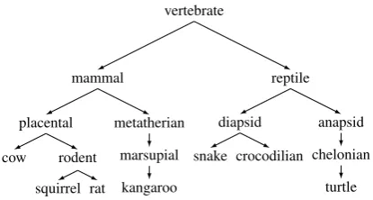
Many tasks in natural language understanding, such as question answering, information extrac-tion, and textual entailment, benefit from lexical semantic information in the form of types and hy-pernyms. A recent example is IBM’s Jeopardy! system Watson (Ferrucci et al., 2010), which used type information to restrict the set of answer can-didates. Information of this sort is present in term taxonomies (e.g., Figure 1), ontologies, and the-sauri. However, currently available taxonomies such as WordNet are incomplete in coverage (Pen-nacchiotti and Pantel, 2006; Hovy et al., 2009), unavailable in many domains and languages, and
vertebrate
mammal
placental
cow rodent squirrel rat
metatherian
marsupial
kangaroo
reptile
diapsid
snake crocodilian
anapsid
chelonian
turtle
[image:1.595.311.519.207.318.2]1
Figure 1: An excerpt of WordNet’s vertebrates taxonomy.
time-intensive to create or extend manually. There has thus been considerable interest in building lex-ical taxonomies automatlex-ically.
In this work, we focus on the task of taking col-lections of terms as input and predicting a com-plete taxonomy structure over them as output. Our model takes a loglinear form and is represented using a factor graph that includes both 1st-order scoring factors on directed hypernymy edges (a parent and child in the taxonomy) and 2nd-order scoring factors on sibling edge pairs (pairs of hy-pernym edges with a shared parent), as well as in-corporating a global (directed spanning tree) struc-tural constraint. Inference for both learning and decoding uses structured loopy belief propagation (BP), incorporating standard spanning tree algo-rithms (Chu and Liu, 1965; Edmonds, 1967; Tutte, 1984). The belief propagation approach allows us to efficiently and effectively incorporate hetero-geneous relational evidence via hypernymy and siblinghood (e.g., coordination) cues, which we capture by semantic features based on simple sur-face patterns and statistics from Webn-grams and Wikipedia abstracts. We train our model to max-imize the likelihood of existing example ontolo-gies using stochastic optimization, automatically learning the most useful relational patterns for full taxonomy induction.
As an example of the relational patterns that our
system learns, suppose we are interested in build-ing a taxonomy for types of mammals (see Fig-ure 1). Frequent attestation of hypernymy patterns likerat is a rodentin large corpora is a strong sig-nal of the link rodent → rat. Moreover, sibling or coordination cues like either rats or squirrels suggest that rat is a sibling of squirrel and adds evidence for the links rodent → rat and rodent
→ squirrel. Our supervised model captures ex-actly these types of intuitions by automatically dis-covering such heterogeneous relational patterns as features (and learning their weights) on edges and on sibling edge pairs, respectively.
There have been several previous studies on taxonomy induction. e.g., the incremental tax-onomy induction system of Snow et al. (2006), the longest path approach of Kozareva and Hovy (2010), and the maximum spanning tree (MST) approach of Navigli et al. (2011) (see Section 4 for a more detailed overview). The main contribution of this work is that we present the first discrimina-tively trained, structured probabilistic model over the full space of taxonomy trees, using a struc-tured inference procedure through both the learn-ing and decodlearn-ing phases. Our model is also the first to directly learn relational patterns as part of the process of training an end-to-end taxonomic induction system, rather than using patterns that were hand-selected or learned via pairwise clas-sifiers on manually annotated co-occurrence pat-terns. Finally, it is the first end-to-end (i.e., non-incremental) system to include sibling (e.g., coor-dination) patterns at all.
We test our approach in two ways. First, on the task of recreating fragments of WordNet, we achieve a 51% error reduction on ancestor-based F1 over a chance baseline, including a 15% error reduction due to the non-hypernym-factored sib-ling features. Second, we also compare to the re-sults of Kozareva and Hovy (2010) by predicting the large animal subtree of WordNet. Here, we get up to 29% relative error reduction on ancestor-based F1. We note that our approach falls at a different point in the space of performance trade-offs from past work – by producing complete, highly articulated trees, we naturally see a more even balance between precision and recall, while past work generally focused on precision.1 To
1While different applications will value precision and
recall differently, and past work was often intentionally precision-focused, it is certainly the case that an ideal solu-tion would maximize both.
avoid presumption of a single optimal tradeoff, we also present results for precision-based decoding, where we trade off recall for precision.
2 Structured Taxonomy Induction
Given an input term set x = {x1, x2, . . . , xn},
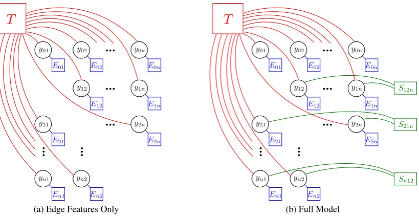
we wish to compute the conditional distribution over taxonomy treesy. This distributionP(y|x) is represented using the graphical model formu-lation shown in Figure 2. A taxonomy treey is composed of a set of indicator random variables yij (circles in Figure 2), where yij = ON means
that xi is the parent of xj in the taxonomy tree
(i.e. there exists a directed edge from xi to xj).
One such variable exists for each pair(i, j) with 0≤i≤n,1≤j ≤n, andi6=j.2
In a factor graph formulation, a set of factors (squares and rectangles in Figure 2) determines the probability of each possible variable assignment. Each factorF has an associated scoring function φF, with the probability of a total assignment
de-termined by the product of all these scores: P(y|x)∝Y
F
φF(y) (1)
2.1 Factor Types
In the models we present here, there are three types of factors: EDGEfactors that score
individ-ual edges in the taxonomy tree, SIBLING factors
that score pairs of edges with a shared parent, and a global TREE factor that imposes the structural
constraint thatyform a legal taxonomy tree.
EDGE Factors. For each edge variable yij in
the model, there is a corresponding factor Eij
(small blue squares in Figure 2) that depends only on yij. We score each edge by extracting a set
of features f(xi, xj) and weighting them by the
(learned) weight vectorw. So, the factor scoring function is:
φEij(yij) = (
exp(w·f(xi, xj)) yij =ON exp(0) = 1 yij =OFF
SIBLING Factors. Our second model also
in-cludes factors that permit 2nd-order features look-ing at terms that are sibllook-ings in the taxonomy tree. For each triple (i, j, k) with i 6= j, i 6= k, and j < k,3we have a factorSijk(green rectangles in
2We assume a special dummy root symbolx0.
3The ordering of the siblings xj and xk doesn’t
y01 y02 y0n
y1n
y12
y21 y2n
yn1 yn2
E02
E01 E0n
E1n E12
E21 E2n
En1 En2
T
(a) Edge Features Only
y01 y02 y0n
y1n
y12
y21 y2n
yn1 yn2
E02
E01 E0n
E1n E12
E21 E2n
En1 En2
S12n
S21n
Sn12
T
[image:3.595.99.509.61.273.2](b) Full Model
Figure 2: Factor graph representation of our model, both without (a) and with (b) SIBLINGfactors.
Figure 2b) that depends on yij andyik, and thus
can be used to encode features that should be ac-tive wheneverxj andxkshare the same parent,xi.
The scoring function is similar to the one above:
φSijk(yij, yik) =
(
exp(w·f(xi, xj, xk)) yij=yik=ON
1 otherwise
TREE Factor. Of course, not all variable as-signments y form legal taxonomy trees (i.e., di-rected spanning trees). For example, the assign-ment∀i, j, yij = ONmight get a high score, but
would not be a valid output of the model. Thus, we need to impose a structural constraint to ensure that such illegal variable assignments are assigned 0 probability by the model. We encode this in our factor graph setting using a single global factorT (shown as a large red square in Figure 2) with the following scoring function:
φT(y) =
(
1 yforms a legal taxonomy tree 0 otherwise
Model.For a given global assignmenty, let
f(y) = X i,j yij=ON
f(xi, xj) +
X
i,j,k yij=yik=ON
f(xi, xj, xk)
Note that by substituting our model’s factor scor-ing functions into Equation 1, we get:
P(y|x)∝ (
exp(w·f(y)) yis a tree
0 otherwise
Thus, our model has the form of a standard loglin-ear model with feature functionf.
2.2 Inference via Belief Propagation
With the model defined, there are two main in-ference tasks we wish to accomplish: computing expected feature counts and selecting a particular taxonomy tree for a given set of input terms (de-coding). As an initial step to each of these pro-cedures, we wish to compute the marginal prob-abilities of particular edges (and pairs of edges) being on. In a factor graph, the natural infer-ence procedure for computing marginals is belief propagation. Note that finding taxonomy trees is a structurally identical problem to directed span-ning trees (and thereby non-projective dependency parsing), for which belief propagation has previ-ously been worked out in depth (Smith and Eisner, 2008). Therefore, we will only briefly sketch the procedure here.
Belief propagation is a general-purpose infer-ence method that computes marginals via directed messages passed from variables to adjacent fac-tors (and vice versa) in the factor graph. These messages take the form of (possibly unnormal-ized) distributions over values of the variable. The two types of messages (variable to factor or fac-tor to variable) have mutually recursive defini-tions. The message from a factorF to an adjacent variable V involves a sum over all possible val-ues of every other variable thatF touches. While the EDGEand SIBLINGfactors are simple enough
How-ever, due to the structure of that particular factor, all of its outgoing messages can be computed si-multaneously inO(n3)time via an efficient
adap-tation of Kirchhoff’s Matrix Tree Theorem (MTT) (Tutte, 1984) which computes partition functions and marginals for directed spanning trees.
Once message passing is completed, marginal beliefs are computed by merely multiplying to-gether all the messages received by a particular variable or factor.
2.2.1 Loopy Belief Propagation
Looking closely at Figure 2a, one can observe that the factor graph for the first version of our model, containing only EDGEand TREE factors,
is acyclic. In this special case, belief propagation is exact: after one round of message passing, the beliefs computed (as discussed in Section 2.2) will be the true marginal probabilities under the cur-rent model. However, in the full model, shown in Figure 2b, the SIBLING factors introduce
cy-cles into the factor graph, and now the messages being passed around often depend on each other and so they will change as they are recomputed. The process of iteratively recomputing messages based on earlier messages is known asloopybelief propagation. This procedure only finds approx-imate marginal beliefs, and is not actually guar-anteed to converge, but in practice can be quite effective for finding workable marginals in mod-els for which exact inference is intractable, as is the case here. All else equal, the more rounds of message passing that are performed, the closer the computed marginal beliefs will be to the true marginals, though in practice, there are usually di-minishing returns after the first few iterations. In our experiments, we used a fairly conservative up-per bound of 20 iterations, but in most cases, the messages converged much earlier than that.
2.3 Training
We used gradient-based maximum likelihood training to learn the model parametersw. Since our model has a loglinear form, the derivative of w with respect to the likelihood objective is computed by just taking the gold feature vec-tor and subtracting the vecvec-tor of expected feature counts. For computing expected counts, we run belief propagation until completion and then, for each factor in the model, we simply read off the marginal probability of that factor being active (as computed in Section 2.2), and accumulate a
par-tial count for each feature that is fired by that fac-tor. This method of computing the gradient can be incorporated into any gradient-based optimizer in order to learn the weightsw. In our experiments we used AdaGrad (Duchi et al., 2011), an adaptive subgradient variant of standard stochastic gradient ascent for online learning.
2.4 Decoding
Finally, once the model parameters have been learned, we want to use the model to find taxon-omy trees for particular sets of input terms. Note that if we limit our scores to be edge-factored, then finding the highest scoring taxonomy tree becomes an instance of the MST problem (also known as the maximum arborescence problem for the directed case), which can be solved effi-ciently inO(n2)quadratic time (Tarjan, 1977)
us-ing the greedy, recursive Chu-Liu-Edmonds algo-rithm (Chu and Liu, 1965; Edmonds, 1967).4
Since the MST problem can be solved effi-ciently, the main challenge becomes finding a way to ensure that our scores are edge-factored. In the first version of our model, we could simply set the score of each edge to bew·f(xi, xj), and the MST
recovered in this way would indeed be the high-est scoring tree: arg maxyP(y|x). However, this
straightforward approach doesn’t apply to the full model which also uses sibling features. Hence, at decoding time, we instead start out by once more using belief propagation to find marginal beliefs, and then set the score of each edge to be its belief odds ratio: bbYij(ON)
Yij(OFF).
5
3 Features
While spanning trees are familiar from non-projective dependency parsing, features based on the linear order of the words or on lexical
identi-4See Georgiadis (2003) for a detailed algorithmic proof,
and McDonald et al. (2005) for an illustrative example. Also, we constrain the Chu-Liu-Edmonds MST algorithm to out-put onlysingle-rootMSTs, where the (dummy) root has ex-actly one child (Koo et al., 2007), because multi-root span-ning ‘forests’ are not applicable to our task.
Also, note that we currently assume one node per term. We are following the task description from previous work where the goal is to create a taxonomy for a specific domain (e.g., animals). Within a specific domain, terms typically just have a single sense. However, our algorithms could certainly be adapted to the case of multiple term senses (by treating the different senses as unique nodes in the tree) in future work.
5The MST that is found using these edge scores is actually
ties or syntactic word classes, which are primary drivers for dependency parsing, are mostly unin-formative for taxonomy induction. Instead, induc-ing taxonomies requires world knowledge to cap-ture the semantic relations between various unseen terms. For this, we use semantic cues to hyper-nymy and siblinghood via features on simple sur-face patterns and statistics in large text corpora. We fire features on both the edge and the sibling factors. We first describe all the edge features in detail (Section 3.1 and Section 3.2), and then briefly describe the sibling features (Section 3.3), which are quite similar to the edge ones.
For each edge factorEij, which represents the
potential parent-child term pair (xi, xj), we add
the surface and semantic features discussed below. Note that since edges are directed, we have sepa-rate features for the factorsEij versusEji.
3.1 Surface Features
Capitalization: Checks which of xi and xj are
capitalized, with one feature for each value of the tuple (isCap(xi), isCap(xj)). The intuition is that
leaves of a taxonomy are often proper names and hence capitalized, e.g., (bison, American bison). Therefore, the feature for (true, false) (i.e., parent capitalized but not the child) gets a substantially negative weight.
Ends with: Checks ifxjends withxi, or not. This
captures pairs such as (fish, bony fish) in our data.
Contains: Checks ifxj containsxi, or not. This
captures pairs such as (bird, bird of prey).
Suffix match: Checks whether the k-length suf-fixes of xi and xj match, or not, for k = 1,2, . . . ,7.
LCS: We compute the longest common substring of xi and xj, and create indicator features for
rounded-off and binned values of|LCS|/((|xi|+ |xj|)/2).
Length difference: We compute the signed length difference between xj andxi, and create
indica-tor features for rounded-off and binned values of (|xj| − |xi|)/((|xi|+|xj|)/2). Yang and Callan
(2009) use a similar feature.
3.2 Semantic Features 3.2.1 Webn-gram Features
Patterns and counts: Hypernymy for a term pair (P=xi, C=xj) is often signaled by the presence
of surface patterns like C is a P, P such as C
in large text corpora, an observation going back to Hearst (1992). For each potential parent-child edge (P=xi, C=xj), we mine the top k strings
(based on count) in which both xi and xj occur
(we usek=200). We collect patterns in both tions, which allows us to judge the correct direc-tion of an edge (e.g.,C is a Pis a positive signal for hypernymy whereasP is a Cis a negative sig-nal).6 Next, for each pattern in this top-klist, we compute its normalized pattern count c, and fire an indicator feature on the tuple (pattern, t), for all thresholds t (in a fixed set) s.t. c ≥ t. Our supervised model then automatically learns which patterns are good indicators of hypernymy.
Pattern order: We add features on the order (di-rection) in which the pair(xi, xj)found a pattern
(in its top-klist) – indicator features for boolean values of the four cases:P . . . C,C . . . P, neither direction, and both directions. Ritter et al. (2009) used the ‘both’ case of this feature.
Individual counts: We also compute the indi-vidual Web-scale term counts cxi and cxj, and
add a comparison feature (cxi>cxj), plus features
on values of the signed count difference (|cxi| −
|cxj|)/((|cxi|+|cxj|)/2), after rounding off, and
binning at multiple granularities. The intuition is that this feature could learn whether the relative popularity of the terms signals their hypernymy di-rection.
3.2.2 Wikipedia Abstract Features
The Webn-grams corpus has broad coverage but is limited to up to5-grams, so it may not contain pattern-based evidence for various longer multi-word terms and pairs. Therefore, we supplement it with a full-sentence resource, namelyWikipedia abstracts, which are concise descriptions (hence useful to signal hypernymy) of a large variety of world entities.
Presence and distance: For each potential edge (xi, xj), we mine patterns from all abstracts in
which the two terms co-occur in either order, al-lowing a maximum term distance of20 (because beyond that, co-occurrence may not imply a rela-tion). We add a presence feature based on whether the process above found at least one pattern for that term pair, or not. We also fire features on the value of the minimum distancedmin at which
6We also allow patterns with surrounding words, e.g.,the
the two terms were found in some abstract (plus thresholded versions).
Patterns: For each term pair, we take the top-k0
patterns (based on count) of length up to l from its full list of patterns, and add an indicator feature on each pattern string (without the counts). We use k0=5,l=10. Similar to the Webn-grams case, we
also fire Wikipedia-based pattern order features.
3.3 Sibling Features
We also incorporate similar features on sibling factors. For each sibling factor Sijk which
rep-resents the potential parent-children term triple (xi, xj, xk), we consider the potential sibling term
pair (xj, xk). Siblinghood for this pair would be
indicated by the presence of surface patterns such aseither C1or C2,C1is similar to C2in large
cor-pora. Hence, we fire Webn-gram pattern features and Wikipedia presence, distance, and pattern fea-tures, similar to those described above, on each potential sibling term pair.7 The main difference here from the edge factors is that the sibling fac-tors are symmetric (in the sense thatSijkis
redun-dant toSikj) and hence the patterns are undirected.
Therefore, for each term pair, we first symmetrize the collected Webn-grams and Wikipedia patterns by accumulating the counts of symmetric patterns likerats or squirrelsandsquirrels or rats.8
4 Related Work
In our work, we assume a known term set and do not address the problem of extracting related terms from text. However, a great deal of past work has considered automating this process, typ-ically taking one of two major approaches. The clustering-based approach (Lin, 1998; Lin and Pantel, 2002; Davidov and Rappoport, 2006; Ya-mada et al., 2009) discovers relations based on the assumption that similar concepts appear in
sim-7One can also add features on the full triple(xi, xj, xk)
but most such features will be sparse.
8All the patterns and counts for our Web and Wikipedia
edge and sibling features described above are extracted after stemming the words in the terms, then-grams, and the ab-stracts (using the Porter stemmer). Also, we threshold the features (to prune away the sparse ones) by considering only those that fire for at leastttrees in the training data (t= 4in our experiments).
Note that one could also add various complementary types of useful features presented by previous work, e.g., bootstrap-ping using syntactic heuristics (Phillips and Riloff, 2002), dependency patterns (Snow et al., 2006), doubly anchored patterns (Kozareva et al., 2008; Hovy et al., 2009), and Web definition classifiers (Navigli et al., 2011).
ilar contexts (Harris, 1954). The pattern-based approach uses special lexico-syntactic patterns to extract pairwise relation lists (Phillips and Riloff, 2002; Girju et al., 2003; Pantel and Pennacchiotti, 2006; Suchanek et al., 2007; Ritter et al., 2009; Hovy et al., 2009; Baroni et al., 2010; Ponzetto and Strube, 2011) and semantic classes or class-instance pairs (Riloff and Shepherd, 1997; Katz and Lin, 2003; Pas¸ca, 2004; Etzioni et al., 2005; Talukdar et al., 2008).
We focus on the second step of taxonomy induc-tion, namely the structured organization of terms into a complete and coherent tree-like hierarchy.9 Early work on this task assumes a starting par-tial taxonomy and inserts missing terms into it. Widdows (2003) place unknown words into a re-gion with the most semantically-similar neigh-bors. Snow et al. (2006) add novel terms by greed-ily maximizing the conditional probability of a set of relational evidence given a taxonomy. Yang and Callan (2009) incrementally cluster terms based on a pairwise semantic distance. Lao et al. (2012) extend a knowledge base using a random walk model to learn binary relational inference rules.
However, the task of inducing full taxonomies without assuming a substantial initial partial tax-onomy is relatively less well studied. There is some prior work on the related task of hierarchical clustering, or grouping together of semantically related words (Cimiano et al., 2005; Cimiano and Staab, 2005; Poon and Domingos, 2010; Fountain and Lapata, 2012). The task we focus on, though, is the discovery of direct taxonomic relationships (e.g., hypernymy) between words.
We know of two closely-related previous sys-tems, Kozareva and Hovy (2010) and Navigli et al. (2011), that build full taxonomies from scratch. Both of these systems use a process that starts by finding basic level terms (leaves of the fi-nal taxonomy tree, typically) and then using re-lational patterns (hand-selected ones in the case of Kozareva and Hovy (2010), and ones learned sep-arately by a pairwise classifier on manually anno-tated co-occurrence patterns for Navigli and Ve-lardi (2010), Navigli et al. (2011)) to find interme-diate terms and all the attested hypernymy links between them.10 To prune down the resulting
tax-9Determining the set of input terms is orthogonal to our
work, and our method can be used in conjunction with vari-ous term extraction approaches described above.
10Unlike our system, which assumes a complete set of
onomy graph, Kozareva and Hovy (2010) use a procedure that iteratively retains the longest paths between root and leaf terms, removing conflicting graph edges as they go. The end result is acyclic, though not necessarily a tree; Navigli et al. (2011) instead use the longest path intuition to weight edges in the graph and then find the highest weight taxonomic tree using a standard MST algorithm.
Our work differs from the two systems above in that ours is the first discriminatively trained, structured probabilistic model over the full space of taxonomy trees that uses structured inference via spanning tree algorithms (MST and MTT) through both the learning and decoding phases. Our model also automatically learns relational pat-terns as a part of the taxonomic training phase, in-stead of relying on hand-picked rules or pairwise classifiers on manually annotated co-occurrence patterns, and it is the first end-to-end (i.e., non-incremental) system to include heterogeneous re-lational information via sibling (e.g., coordina-tion) patterns.
5 Experiments
5.1 Data and Experimental Regime
We considered two distinct experimental setups, one that illustrates the general performance of our model by reproducing various medium-sized WordNet domains, and another that facilitates comparison to previous work by reproducing the much largeranimalsubtree provided by Kozareva and Hovy (2010).
General setup: In order to test the accuracy of structured prediction on medium-sized full-domain taxonomies, we extracted from WordNet 3.0 all bottomed-out full subtrees which had a tree-height of 3 (i.e., 4 nodes from root to leaf), and contained (10, 50] terms.11 This gives us 761 non-overlapping trees, which we partition into
both these systems include term discovery in the taxonomy building process.
11Subtrees that had a smaller or larger tree height were
dis-carded in order to avoid overlap between the training and test divisions. This makes it a muchstricter settingthan other tasks such as parsing, which usually has repeated sentences, clauses and phrases between training and test sets.
To project WordNet synsets to terms, we used the first (most frequent) term in each synset. A few WordNet synsets have multiple parents so we only keep the first of each such pair of overlapping trees. We also discard a few trees with duplicate terms because this is mostly due to the projection of different synsets to the same term, and theoretically makes the tree a graph.
70/15/15% (533/114/114 trees) train/dev/test sets.
Comparison setup: We also compare our method (as closely as possible) with related previous work by testing on the much largeranimalsubtree made available by Kozareva and Hovy (2010), who cre-ated this dataset by selecting a set of ‘harvested’ terms and retrieving all the WordNet hypernyms between each input term and the root (i.e., an-imal), resulting in ∼700 terms and ∼4,300 is-a ancestor-child links.12 Our training set for this an-imal test case was generated from WordNet us-ing the followus-ing process: First, we strictly re-move thefullanimal subtree from WordNet in or-der to avoid any possible overlap with the test data. Next, we create random 25-sized trees by picking random nodes as singleton trees, and repeatedly adding child edges from WordNet to the tree. This process gives us a total of∼1600 training trees.13
Feature sources: The n-gram semantic features are extracted from the Google n-grams corpus (Brants and Franz, 2006), a large collection of English n-grams (forn = 1 to 5) and their fre-quencies computed from almost 1 trillion tokens (95 billion sentences) of Web text. The Wikipedia abstracts are obtained via the publicly available dump, which contains almost ∼4.1 million ar-ticles.14 Preprocessing includes standard XML parsing and tokenization. Efficient collection of feature statistics is important because these must be extracted for millions of query pairs (for each potential edge and sibling pair in each term set). For this, we use a hash-trie on term pairs (sim-ilar to that of Bansal and Klein (2011)), and scan once through then-gram (or abstract) set, skipping manyn-grams (or abstracts) based on fast checks of missing unigrams, exceeding length, suffix mis-matches, etc.
5.2 Evaluation Metric
Ancestor F1: Measures the precision, recall, and F1 = 2P R/(P+R)of correctly predicted
ances-12This is somewhat different from our general setup where
we work with any given set of terms; they start with a large set of leaves which have substantial Web-based relational information based on their selected, hand-picked patterns. Their data is available athttp://www.isi.edu/˜kozareva/ downloads.html.
13We tried this training regimen as different from that of
the general setup (which contains only bottomed-out sub-trees), so as to match theanimaltest tree, which is of depth 12 and has intermediate nodes from higher up in WordNet.
System P R F1 Edges-Only Model
Baseline 5.9 8.3 6.9
Surface Features 17.5 41.3 24.6 Semantic Features 37.0 49.1 42.2 Surface+Semantic 41.1 54.4 46.8
Edges + Siblings Model
Surface+Semantic 53.1 56.6 54.8
[image:8.595.76.289.62.194.2]Surface+Semantic (Test) 48.0 55.2 51.4
Table 1: Main results on our general setup. On the devel-opment set, we present incremental results on the edges-only model where we start with the chance baseline, then use sur-face features only, semantic features only, and both. Finally, we add sibling factors and features to get results for the full, edges+siblings model with all features, and also report the final test result for this setting.
tors, i.e., pairwiseis-arelations:
P =|isagold|isa∩ isapredicted|
predicted| , R=
|isagold ∩ isapredicted|
|isagold|
5.3 Results
Table 1 shows our main results for ancestor-based evaluation on the general setup. We present a de-velopment set ablation study where we start with the edges-only model (Figure 2a) and its random tree baseline (which chooses any arbitrary span-ning tree for the term set). Next, we show results on the edges-only model with surface features (Section 3.1), semantic features (Section 3.2), and both. We see that both surface and semantic fea-tures make substantial contributions, and they also stack. Finally, we add the sibling factors and fea-tures (Figure 2b, Section 3.3), which further im-proves the results significantly (8% absolute and 15% relative error reduction over the edges-only results on the ancestor F1 metric). The last row shows the final test set results for the full model with all features.
Table 2 shows our results for comparison to the larger animal dataset of Kozareva and Hovy (2010).15 In the table, ‘Kozareva2010’ refers to Kozareva and Hovy (2010) and ‘Navigli2011’ refers to Navigli et al. (2011).16 For
appropri-15These results are for the 1st order model due to the scale
of the animal taxonomy (∼700 terms). For scaling the 2nd order sibling model, one can use approximations, e.g., prun-ing the set of siblprun-ing factors based on 1st order link marginals, or a hierarchical coarse-to-fine approach based on taxonomy induction on subtrees, or a greedy approach of adding a few sibling factors at a time. This is future work.
16The Kozareva and Hovy (2010) ancestor results are
ob-tained by using the output files provided on their webpage.
System P R F1
Previous Work
Kozareva2010 98.6 36.2 52.9
Navigli2011?? 97.0?? 43.7?? 60.3??
This Paper
Fixed Prediction 84.2 55.1 66.6
Free Prediction 79.3 49.0 60.6
Table 2: Comparison results on the animal dataset of Kozareva and Hovy (2010). Here, ‘Kozareva2010’ refers to Kozareva and Hovy (2010) and ‘Navigli2011’ refers to Nav-igli et al. (2011). For appropriate comparison to each previ-ous work, we show our results both for the ‘Fixed Prediction’ setup, which assumes the true root and leaves, and for the ‘Free Prediction’ setup, which doesn’t assume any prior in-formation. The??results of Navigli et al. (2011) represent a different ground-truth data condition, making them incompa-rable to our results; see Section 5.3 for details.
ate comparison to each previous work, we show results for two different setups. The first setup ‘Fixed Prediction’ assumes that the model knows the true root and leaves of the taxonomy to provide for a somewhat fairer comparison to Kozareva and Hovy (2010). We get substantial improvements on ancestor-based recall and F1 (a 29% relative error reduction). The second setup ‘Free Predic-tion’ assumes no prior knowledge and predicts the full tree (similar to the general setup case). On this setup, we do compare as closely as possible to Navigli et al. (2011) and see a small gain in F1, but regardless, we should note that their results are incomparable (denoted by?? in Table 2) because they have a different ground-truth data condition: their definition and hypernym extraction phase in-volves using the Googledefinekeyword, which often returns WordNet glosses itself.
We note that previous work achieves higher an-cestor precision, while our approach achieves a more even balance between precision and recall. Of course, precision and recall should both ide-ally be high, even if some applications weigh one over the other. This is why our tuning optimized for F1, which represents a neutral combination for comparison, but other Fα metrics could also
[image:8.595.305.528.62.167.2]Hypernymy features C and other P >P>C
C , P of C is a P
C , a P P , including C
C or other P P ( C
C : a P C , american P C - like P C , the P
Siblinghood features C1and C2 C1, C2(
C1or C2 of C1and / or C2
, C1, C2and either C1 or C2
[image:9.595.75.289.61.231.2]the C1/ C2 <s>C1and C2</s>
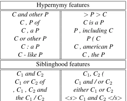
Table 3: Examples of high-weighted hypernymy and sibling-hood features learned during development.
butterfly
copper American copper
hairstreak Strymon melinus
admiral
white admiral
[image:9.595.308.525.64.129.2]1
Figure 3: Excerpt from the predictedbutterflytree. The terms attached erroneously according to WordNet are marked in red and italicized.
6 Analysis
Table 3 shows some of the hypernymy and sibling-hood features given highest weight by our model (in general-setup development experiments). The training process not only rediscovers most of the standard Hearst-style hypernymy patterns (e.g.,C and other P, C is a P), but also finds various novel, intuitive patterns. For example, the pattern C, american P is prominent because it captures pairs like Lemmon, american actor and Bryon, american politician, etc. Another pattern>P > Ccaptures webpage navigation breadcrumb trails (representing category hierarchies). Similarly, the algorithm also discovers useful siblinghood fea-tures, e.g.,either C1or C2,C1and / or C2, etc.
Finally, we look at some specific output errors to give as concrete a sense as possible of some sys-tem confusions, though of course any hand-chosen examples must be taken as illustrative. In Figure 3, we attach white admiral to admiral, whereas the gold standard makes these two terms siblings. In reality, however, white admirals are indeed a species of admirals, so WordNet’s ground truth turns out to be incomplete. Another such example is that we placelogistic assessment in the
evalu-bottle
flask
vacuum flask thermos Erlenmeyer flask
wine bottle jeroboam
1
Figure 4: Excerpt from the predictedbottletree. The terms attached erroneously according to WordNet are marked in red and italicized.
ationsubtree ofjudgment, but WordNet makes it a direct child ofjudgment. However, other dictio-naries do consider logistic assessments to be eval-uations. Hence, this illustrates that there may be more than one right answer, and that the low re-sults on this task should only be interpreted as such. In Figure 4, our algorithm did not recog-nize that thermosis a hyponym of vacuum flask, and thatjeroboamis a kind of wine bottle. Here, our Webn-grams dataset (which only contains fre-quent n-grams) and Wikipedia abstracts do not suffice and we would need to add richer Web data for such world knowledge to be reflected in the features.
7 Conclusion
Our approach to taxonomy induction allows het-erogeneous information sources to be combined and balanced in an error-driven way. Direct indi-cators of hypernymy, such as Hearst-style context patterns, are the core feature for the model and are discovered automatically via discriminative train-ing. However, other indicators, such as coordina-tion cues, can indicate that two words might be siblings, independently of what their shared par-ent might be. Adding second-order factors to our model allows these two kinds of evidence to be weighed and balanced in a discriminative, struc-tured probabilistic framework. Empirically, we see substantial gains (in ancestor F1) from sibling features, and also over comparable previous work. We also present results on the precision and recall trade-offs inherent in this task.
Acknowledgments
[image:9.595.76.289.280.344.2]References
Mohit Bansal and Dan Klein. 2011. Web-scale
fea-tures for full-scale parsing. InProceedings of ACL.
Marco Baroni, Brian Murphy, Eduard Barbu, and Mas-simo Poesio. 2010. Strudel: A corpus-based
seman-tic model based on properties and types. Cognitive
Science, 34(2):222–254.
Thorsten Brants and Alex Franz. 2006. The Google
Web 1T 5-gram corpus version 1.1.LDC2006T13.
Yoeng-Jin Chu and Tseng-Hong Liu. 1965. On the
shortest arborescence of a directed graph. Science
Sinica, 14(1396-1400):270.
Philipp Cimiano and Steffen Staab. 2005. Learning concept hierarchies from text with a guided
agglom-erative clustering algorithm. In Proceedings of the
ICML 2005 Workshop on Learning and Extending Lexical Ontologies with Machine Learning
Meth-ods.
Philipp Cimiano, Andreas Hotho, and Steffen Staab. 2005. Learning concept hierarchies from text
cor-pora using formal concept analysis. Journal of
Arti-ficial Intelligence Research, 24(1):305–339.
Dmitry Davidov and Ari Rappoport. 2006. Effi-cient unsupervised discovery of word categories us-ing symmetric patterns and high frequency words.
InProceedings of COLING-ACL.
John Duchi, Elad Hazan, and Yoram Singer. 2011. Adaptive subgradient methods for online learning
and stochastic optimization. The Journal of
Ma-chine Learning Research, 12:2121–2159.
Jack Edmonds. 1967. Optimum branchings. Journal
of Research of the National Bureau of Standards B,
71:233–240.
Oren Etzioni, Michael Cafarella, Doug Downey, Ana-Maria Popescu, Tal Shaked, Stephen Soderland, Daniel S. Weld, and Alexander Yates. 2005. Un-supervised named-entity extraction from the Web:
An experimental study. Artificial Intelligence,
165(1):91–134.
David Ferrucci, Eric Brown, Jennifer Chu-Carroll, James Fan, David Gondek, Aditya A Kalyanpur, Adam Lally, J William Murdock, Eric Nyberg, John Prager, Nico Schlaefer, and Chris Welty. 2010. Building watson: An overview of the DeepQA
project. AI magazine, 31(3):59–79.
Trevor Fountain and Mirella Lapata. 2012. Taxonomy
induction using hierarchical random graphs. In
Pro-ceedings of NAACL.
Leonidas Georgiadis. 2003. Arborescence
optimiza-tion problems solvable by edmonds algorithm.
The-oretical Computer Science, 301(1):427–437.
Roxana Girju, Adriana Badulescu, and Dan Moldovan. 2003. Learning semantic constraints for the
auto-matic discovery of part-whole relations. In
Proceed-ings of NAACL.
Joshua Goodman. 1996. Parsing algorithms and
met-rics. InProceedings of ACL.
Zellig Harris. 1954. Distributional structure. Word,
10(23):146–162.
Marti Hearst. 1992. Automatic acquisition of
hy-ponyms from large text corpora. InProceedings of
COLING.
Eduard Hovy, Zornitsa Kozareva, and Ellen Riloff. 2009. Toward completeness in concept extraction
and classification. InProceedings of EMNLP.
Boris Katz and Jimmy Lin. 2003. Selectively using re-lations to improve precision in question answering.
In Proceedings of the Workshop on NLP for
Ques-tion Answering (EACL 2003).
Terry Koo, Amir Globerson, Xavier Carreras, and Michael Collins. 2007. Structured prediction
mod-els via the matrix-tree theorem. In Proceedings of
EMNLP-CoNLL.
Zornitsa Kozareva and Eduard Hovy. 2010. A
semi-supervised method to learn and construct
tax-onomies using the Web. InProceedings of EMNLP.
Zornitsa Kozareva, Ellen Riloff, and Eduard Hovy. 2008. Semantic class learning from the web with
hyponym pattern linkage graphs. InProceedings of
ACL.
Ni Lao, Amarnag Subramanya, Fernando Pereira, and William W. Cohen. 2012. Reading the web with
learned syntactic-semantic inference rules. In
Pro-ceedings of EMNLP.
Dekang Lin and Patrick Pantel. 2002. Concept
discov-ery from text. InProceedings of COLING.
Dekang Lin. 1998. Automatic retrieval and clustering
of similar words. InProceedings of COLING.
Ryan McDonald, Fernando Pereira, Kiril Ribarov, and Jan Hajiˇc. 2005. Non-projective dependency
pars-ing uspars-ing spannpars-ing tree algorithms. InProceedings
of HLT-EMNLP.
Roberto Navigli and Paola Velardi. 2010. Learning word-class lattices for definition and hypernym
ex-traction. InProceedings of the 48th Annual Meeting
of the Association for Computational Linguistics.
Roberto Navigli, Paola Velardi, and Stefano Faralli. 2011. A graph-based algorithm for inducing lexical
taxonomies from scratch. InProceedings of IJCAI.
Patrick Pantel and Marco Pennacchiotti. 2006.
Espresso: Leveraging generic patterns for
automati-cally harvesting semantic relations. InProceedings
Marius Pas¸ca. 2004. Acquisition of categorized named
entities for web search. InProceedings of CIKM.
Marco Pennacchiotti and Patrick Pantel. 2006.
On-tologizing semantic relations. In Proceedings of
COLING-ACL.
William Phillips and Ellen Riloff. 2002. Exploiting strong syntactic heuristics and co-training to learn
semantic lexicons. InProceedings of EMNLP.
Simone Paolo Ponzetto and Michael Strube. 2011. Taxonomy induction based on a collaboratively
built knowledge repository. Artificial Intelligence,
175(9):1737–1756.
Hoifung Poon and Pedro Domingos. 2010.
Unsuper-vised ontology induction from text. InProceedings
of ACL.
Ellen Riloff and Jessica Shepherd. 1997. A corpus-based approach for building semantic lexicons. In
Proceedings of EMNLP.
Alan Ritter, Stephen Soderland, and Oren Etzioni. 2009. What is this, anyway: Automatic hypernym
discovery. InProceedings of AAAI Spring
Sympo-sium on Learning by Reading and Learning to Read.
David A. Smith and Jason Eisner. 2008. Dependency
parsing by belief propagation. In Proceedings of
EMNLP.
Rion Snow, Daniel Jurafsky, and Andrew Y. Ng. 2006. Semantic taxonomy induction from heterogenous
evidence. InProceedings of COLING-ACL.
Fabian M. Suchanek, Gjergji Kasneci, and Gerhard Weikum. 2007. Yago: a core of semantic
knowl-edge. InProceedings of WWW.
Partha Pratim Talukdar, Joseph Reisinger, Marius Pas¸ca, Deepak Ravichandran, Rahul Bhagat, and Fernando Pereira. 2008. Weakly-supervised acqui-sition of labeled class instances using graph random
walks. InProceedings of EMNLP.
Robert E. Tarjan. 1977. Finding optimum branchings.
Networks, 7:25–35.
William T. Tutte. 1984. Graph theory.
Addison-Wesley.
Dominic Widdows. 2003. Unsupervised methods for developing taxonomies by combining syntactic
and statistical information. InProceedings of
HLT-NAACL.
Ichiro Yamada, Kentaro Torisawa, Jun’ichi Kazama, Kow Kuroda, Masaki Murata, Stijn De Saeger, Fran-cis Bond, and Asuka Sumida. 2009. Hypernym dis-covery based on distributional similarity and
hierar-chical structures. InProceedings of EMNLP.
Hui Yang and Jamie Callan. 2009. A metric-based framework for automatic taxonomy induction. In