Exploiting Topic based Twitter Sentiment for Stock Prediction

Proceedings of the 51st Annual Meeting of the Association for Computational Linguistics, pages 24–29, Sofia, Bulgaria, August 4-9 2013. c2013 Association for Computational Linguistics

Exploiting Topic based Twitter Sentiment for Stock Prediction

Jianfeng Si

Arjun Mukherjee

Bing Liu

Qing Li

Huayi Li

Xiaotie Deng

Department of Computer Science, City University of Hong Kong, Hong Kong, China

*

{

thankjeff@gmail.com, qing.li@cityu.edu.hk

}

Department of Computer Science, University of Illinois at Chicago, Chicago, IL 60607, USA

{

arjun4787@gmail.com, liub@cs.uic.edu, lhymvp@gmail.com

}

AIMS Lab, Department of Computer Science, Shanghai Jiaotong University, Shanghai, China

_{deng-xt@cs.sjtu.edu.cn}

Abstract

This paper proposes a technique to leverage topic based sentiments from Twitter to help predict the stock market. We first utilize a con-tinuous Dirichlet Process Mixture model to learn the daily topic set. Then, for each topic we derive its sentiment according to its opin-ion words distributopin-ion to build a sentiment time series. We then regress the stock index and the Twitter sentiment time series to predict the market. Experiments on real-life S&P100 Index show that our approach is effective and performs better than existing state-of-the-art non-topic based methods.

1

Introduction

Social media websites such as Twitter, Facebook, etc., have become ubiquitous platforms for social networking and content sharing. Every day, they generate a huge number of messages, which give researchers an unprecedented opportunity to uti-lize the messages and the public opinions con-tained in them for a wide range of applications (Liu, 2012). In this paper, we use them for the application of stock index time series analysis.

Here are some example tweets upon querying the keyword “$aapl” (which is the stock symbol for Apple Inc.) in Twitter:

1.“Shanghai Oriental Morning Post confirm-ing w Sources that $AAPL TV will debut in May, Prices range from $1600-$3200, but $32,000 for a 50"wow.”

2. “$AAPL permanently lost its bid for a ban on U.S. sales of the Samsung Galaxy Nex-us http://dthin.gs/XqcY74.”

3.“$AAPL is loosing customers. everybody is buying android phones! $GOOG.”

As shown, the retrieved tweets may talk about Apple’s products, Apple’s competition relation-ship with other companies, etc. These messages are often related to people’s sentiments about Apple Inc., which can affect or reflect its stock trading since positive sentiments can impact sales and financial gains. Naturally, this hints that topic based sentiment is a useful factor to consider for stock prediction as they reflect peo-ple’s sentiment on different topics in a certain time frame.

This paper focuses on daily one-day-ahead prediction of stock index based on the temporal characteristics of topics in Twitter in the recent past. Specifically, we propose a non-parametric topic-based sentiment time series approach to analyzing the streaming Twitter data. The key motivation here is that Twitter’s streaming mes-sages reflect fresh sentiments of people which are likely to be correlated with stocks in a short time frame. We also analyze the effect of training window size which best fits the temporal dynam-ics of stocks. Here window size refers to the number of days of tweets used in model building. Our final prediction model is built using vec-tor auvec-toregression (VAR). To our knowledge, this is the first attempt to use non-parametric continuous topic based Twitter sentiments for stock prediction in an autoregressive framework.

2

Related Work

2.1 Market Prediction and Social Media

Stock market prediction has attracted a great deal of attention in the past. Some recent researches suggest that news and social media such as blogs, micro-blogs, etc., can be analyzed to extract pub-lic sentiments to help predict the market (La-vrenko et al., 2000; Schumaker and Chen, 2009). Bollen et al. (2011) used tweet based public mood to predict the movement of Dow Jones

* The work was done when the first author was visiting University of Illinois at Chicago.

Industrial Average index. Ruiz et al. (2012) stud-ied the relationship between Twitter activities and stock market under a graph based view. Feldman et al. (2011) introduced a hybrid ap-proach for stock sentiment analysis based on companies’ news articles.

2.2 Aspect and Sentiment Models

Topic modeling as a task of corpus exploration has attracted significant attention in recent years. One of the basic and most widely used models is Latent Dirichlet Allocation (LDA) (Blei et al., 2003). LDA can learn a predefined number of topics and has been widely applied in its extend-ed forms in sentiment analysis and many other tasks (Mei et al., 2007; Branavan et al., 2008; Lin and He, 2009; Zhao et al., 2010; Wang et al., 2010; Brody and Elhadad, 2010; Jo and Oh, 2011; Moghaddam and Ester, 2011; Sauper et al., 2011; Mukherjee and Liu, 2012; He et al., 2012).

The Dirichlet Processes Mixture (DPM) model is a non-parametric extension of LDA (Teh et al., 2006), which can estimate the number of topics inherent in the data itself. In this work, we em-ploy topic based sentiment analysis using DPM on Twitter posts (or tweets). First, we employ a DPM to estimate the number of topics in the streaming snapshot of tweets in each day.

Next, we build a sentiment time series based on the estimated topics of daily tweets. Lastly, we regress the stock index and the sentiment time series in an autoregressive framework.

3

Model

We now present our stock prediction framework.

3.1 Continuous DPM Model

Comparing to edited articles, it is much harder to preset the number of topics to best fit continuous streaming Twitter data due to the large topic di-versity in tweets. Thus, we resort to a non-parametric approach: the Dirichlet Process Mix-ture (DPM) model, and let the model estimate the number of topics inherent in the data itself.

Mixture model is widely used in clustering and

can be formalized as follows:

∑ ( ) (1)

where is a data point, is its cluster label, K

is the number of topics, ( ) is the sta-tistical (topic) models: * + and is the

component weight satisfying and

∑ .

In our setting of DPM, the number of mixture components (topics) K is unfixed apriori but es-timated from tweets in each day. DPM is defined as in (Neal, 2010):

( )

( ) (2)

where is the parameter of the model that belongs to, and is defined as a Dirichlet Pro-cess with the base measure H and the concentra-tion parameter (Neal, 2010).

We note that neighboring days may share the same or closely related topics because some top-ics may last for a long period of time covering multiple days, while other topics may just last for a short period of time. Given a set of time-stamped tweets, the overall generative process should be dynamic as the topics evolve over time. There are several ways to model this dynamic nature (Sun et al., 2010; Kim and Oh, 2011; Chua and Asur, 2012; Blei and Lafferty, 2006; Wang et al., 2008). In this paper, we follow the approach of Sun et al. (2010) due to its generality and extensibility.

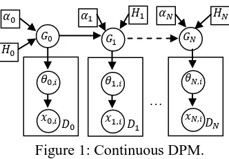
Figure 1 shows the graphical model of our con-tinuous version of DPM (which we call cDPM). As shown, the tweets set is divided into daily based collections: * + * + are the

observed tweets and * + are the model

pa-rameters (latent topics) that generate these tweets. For each subset of tweets, (tweets of day ), we build a DPM on it. For the first day ( ), the model functions the same as a standard DPM, i.e., all the topics use the same base measure,

( ). However, for later days ( ), besides the base measure, ( ), we make use of topics learned from previous days as pri-ors. This ensures smooth topic chains or links (details in §3.2). For efficiency, we only consider topics of one previous day as priors.

We use collapsed Gibbs sampling (Bishop, 2006) for model inference. Hyper-parameters are set to: ; as in (Sun et al., 2010; Teh et al., 2006) which have been shown to work well. Because a tweet has at most 140 characters, we assume that each tweet contains only one topic. Hence, we only need to Figure 1: Continuous DPM.

…

sample the topic assignment for each tweet . According to different situations with respect to a topic’s prior, for each tweet in , the conditional distribution for given all other tweets’ topic assignments, denoted by , can be

summarized as follows:

1. is a new topic: Its candidate priors contain the symmetric base prior ( ) and topics

* + _{learned from}

.

 If takes a symmetric base prior:

( )

( )

( )

∏ ( )

∏ ( ) (3)

where the first part denotes the prior proba-bility according to the Dirichlet Process and the second part is the data likelihood (this interpretation can similarly be applied to the following three equations).

 If takes one topic k from * + as

its prior:

( )

( )

( )

∏ ( ( ) )

∏ ( ( ))

(4)

2. k is an existing topic: We already know its prior.

 If k takes a symmetric base prior:

( )

( _{( )} )

( _{( ) )}

∏ ( )

∏ ( ) (5)

 If k takes topic as its prior: ( )

. _{( )} / . _{( )} /

∏ ( ( ) ) ∏ ( ( ) ) (6)

Notations in the above equations are listed as follows:

 is the number of topics learned in day t-1.  |V| is the vocabulary size.

 is the document length of .

 is the term frequency of word in .

 ( ) is the probability of word in

pre-vious day’s topic k.

 is the number of tweets assigned to topic k

excluding the current one .

 is the term frequency of word in topic k,

with statistic from excluded. While _{( )} denotes the marginalized sum of all words in topic k with statistic from excluded.

Similarly, the posteriors on * ( )+ (topic

word distributions) are given according to their prior situations as follows:

 If topic k takes the base prior:

( ) ( ) ( ( )) ⁄ (7)

where is the frequency of word in topic

k and ( ) is the marginalized sum over all

words.

 otherwise, it is defined recursively as:

( ) ( ( ) ) ( ( ))⁄ (8)

where serves as the topic prior for .

Finally, for each day we estimate the topic weights, as follows:

⁄∑ (9)

where is the number of tweets in topic k.

3.2 Topic-based Sentiment Time Series

Based on an opinion lexicon (a list of positive and negative opinion words, e.g., good and bad), each opinion word, is assigned with a po-larity label ( ) as “+1” if it is positive and “-1” if negative. We spilt each tweet’s text into opin-ion part and non-opinopin-ion part. Only non-opinopin-ion words in tweets are used for Gibbs sampling.

Based on DPM, we learn a set of topics from the non-opinion words space . The correspond-ing tweets’ opinion words share the same topic assignments as its tweet. Then, we compute the posterior on opinion word probability, ( ) for topic analogously to equations (7) and (8). Finally, we define the topic based sentiment score ( ) of topic in day t as a weighted linear combination of the opinion polarity labels:

( ) ∑ ( ) ( ); ( ) , - (10)

According to the generative process of cDPM, topics between neighboring days are linked if a topic k takes another topic as its prior. We regard this as evolution of topic k. Although there may be slight semantic variation, the assumption is reasonable. Then, the sentiment scores for each topic series form the sentiment time series {…,

S(t-1, k), S(t, k), S(t+1, k), ...}.

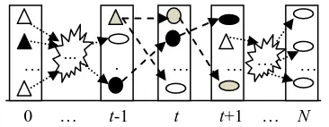
Figure 2 demonstrates the linking process where a triangle denotes a new topic (with base symmetric prior), a circle denotes a middle topic (taking a topic from the previous day as its prior,

0 … t-1 t t+1 … N

Figure 2: Linking the continuous topics via neighboring priors.

Figure 1: Continuous DPM … ...

… .

. .

while also supplying prior for the next day) and an ellipse denotes an end topic (no further topics use it as a prior). In this example, two continuous topic chains or links (via linked priors) exist for the time interval [t-1, t+1]: one in light grey color, and the other in black. As shown, there may be more than one topic chain/link (5-20 in our ex-periments) for a certain time interval1.Thus, we sort multiple sentiment series according to their accumulative weights of topics over each link:

∑ . In our experiments, we try the top five series and use the one that gives the best re-sult, which is mostly the first (top ranked) series with a few exceptions of the second series. The topics mostly focus on hot keywords like: news,

stocknews, earning, report, which stimulate ac-tive discussions on the social media platform.

3.3 Time Series Analysis with VAR

For model building, we use vector autoregression (VAR). The first order (time steps of historical information to use: lag = 1) VAR model for two time series * + and * + is given by:

(11)

where * + are the white noises and * + are model parameters. We use the “dse” library2 in the R

language to fit our VAR model based on least square regression.

Instead of training in one period and predicting over another disjointed period, we use a moving training and prediction process under sliding windows3 (i.e., train in [t, t + w] and predict in-dex on t + w + 1) with two main considerations: Due to the dynamic and random nature of both

the stock market and public sentiments, we are more interested in their short term relationship. Based on the sliding windows, we have more

training and testing points.

Figure 3 details the algorithm for stock index prediction. The accuracy is computed based on the index up and down dynamics, the function

( ) returns True only if (our predic-tion) and (actual value) share the same index up or down direction.

1

The actual topic priors for topic links are governed by the four cases of the Gibbs Sampler.

2

http://cran.r-project.org/web/packages/dse

3

This is similar to the autoregressive moving average (ARMA) models.

4

Dataset

We collected the tweets via Twitter’s REST API for streaming data, using symbols of the Stand-ard & Poor's 100 stocks (S&P100) as keywords. In this study, we focus only on predicting the S&P100 index. The time period of our dataset is between Nov. 2, 2012 and Feb. 7, 2013, which gave us 624782 tweets. We obtained the S&P100 index’s daily close values from Yahoo Finance.

5

Experiment

5.1 Selecting a Sentiment Metric

Bollen et al. (2011) used the mood dimension,

Calm together with the index value itself to pre-dict the Dow Jones Industrial Average. However, their Calm lexicon is not publicly available. We thus are unable to perform a direct comparison with their system. We identified and labeled a

Calm lexicon (words like “anxious”, “shocked”,

“settled” and “dormant”) using the opinion

lexi-con4 of Hu and Liu (2004) and computed the sen-timent score using the method of Bollen et al. (2011) (sentiment ratio). Our pilot experiments showed that using the full opinion lexicon of Hu and Liu (2004) actually performs consistently better than the Calm lexicon. Hence, we use the entire opinion lexicon in Hu and Liu (2004).

5.2 S&P100INDEX Movement Prediction

We evaluate the performance of our method by comparing with two baselines. The first (Index) uses only the index itself, which reduces the VAR model to the univariate autoregressive model (AR), resulting in only one index time series { } in the algorithm of Figure 3.

4

http://cs.uic.edu/~liub/FBS/opinion-lexicon-English.rar

Parameter:

w: training window size; lag: the order of VAR; Input: : the date of time series; { }: sentiment time series; { }: index time series;

Output: prediction accuracy. 1. for t = 0, 1, 2, …, N-w-1 2. {

3. = VAR( , - , -, lag); 4. = .Predict(x[t+w+1-lag, t+w],

y[t+w+1-lag, t+w]); 5. if ( ( ) )

rightNum++; 6. }

7. Accuracy = rightNum / (N-w); 8. Return Accuracy;

Figure 3: Prediction algorithm and accuracy

When considering Twitter sentiments, existing works (Bollen et al., 2011, Ruiz et al., 2012) simply compute the sentiment score as ratio of pos/neg opinion words per day. This generates a lexicon-based sentiment time series, which is then combined with the index value series to give us the second baseline Raw.

In summary, Index uses index only with the AR model while Raw uses index and opinion lexicon based time series. Our cDPM uses index and the proposed topic based sentiment time se-ries. Both Raw and cDPM employ the two di-mensional VAR model. We experiment with dif-ferent lag settings from 1-3 days.

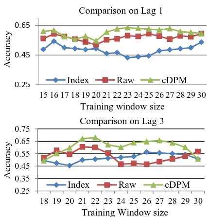
We also experiment with different training window sizes, ranging from 15 - 30 days, and compute the prediction accuracy for each win-dow size. Table 1 shows the respective average and best accuracies over all window sizes for each lag and Table 2 summarizes the pairwise performance improvements of averaged scores over all training window sizes. Figure 4 show the detailed accuracy comparison for lag 1 and lag 3. From Table 1, 2, and Figure 4, we note: i. Topic-based public sentiments from tweets

can improve stock prediction over simple sen-timent ratio which may suffer from backchan-nel noise and lack of focus on prevailing top-ics. For example, on lag 2, Raw performs worse by 8.6% than Index itself.

ii. cDPM outperforms all others in terms of both the best accuracy (lag 3) and the average ac-curacies for different window sizes. The max-imum average improvement reaches 25.0% compared to Index at lag 1 and 15.1% com-pared to Raw at lag 3. This is due to the fact that cDPM learns the topic based sentiments instead of just using the opinion words’ ratio like Raw, and in a short time period, some topics are more correlated with the stock

mar-ket than others. Our proposed sentiment time series using cDPM can capture this phenome-non and also help reduce backchannel noise of raw sentiments.

iii.On average, cDPM gets the best performance for training window sizes within [21, 22], and the best prediction accuracy is 68.0% on win-dow size 22 at lag 3.

6

Conclusions

Predicting the stock market is an important but difficult problem. This paper showed that Twit-ter’s topic based sentiment can improve the pre-diction accuracy beyond existing non-topic based approaches. Specifically, a non-parametric topic-based sentiment time series approach was pro-posed for the Twitter stream. For prediction, vec-tor auvec-toregression was used to regress S&P100 index with the learned sentiment time series. Be-sides the short term dynamics based prediction, we believe that the proposed method can be ex-tended for long range dependency analysis of Twitter sentiments and stocks, which can render deep insights into the complex phenomenon of stock market. This will be part of our future work.

Acknowledgments

This work was supported in part by a grant from the National Science Foundation (NSF) under grant no. IIS-1111092 and a strategic research grant from City University of Hong Kong (pro-ject number: 7002770).

Lag Index Raw cDPM

1 0.48(0.54) 0.57(0.59) 0.60(0.64) 2 0.58(0.65) 0.53(0.62) 0.60(0.63) 3 0.52(0.56) 0.53(0.60) 0.61(0.68)

Table 1: Average (best) accuracies over all training window sizes and different lags 1, 2, 3.

Lag Raw vs. IndexcDPM vs. Index cDPM vs. Raw

1 18.8% 25.0% 5.3%

2 -8.6% 3.4% 13.2%

3 1.9% 17.3% 15.1%

Table 2: Pairwise improvements among Index,

Raw and cDPM averaged over all training win-dow sizes.

Figure 4: Comparison of prediction accuracy of up/down stock index on S&P 100 index for dif-ferent training window sizes.

0.25 0.45 0.65

15 16 17 18 19 20 21 22 23 24 25 26 27 28 29 30

A

cc

u

rac

y

Training window size Comparison on Lag 1

Index Raw cDPM

0.25 0.35 0.45 0.55 0.65 0.75

18 19 20 21 22 23 24 25 26 27 28 29 30

A

cc

u

rac

y

Training Window size Comparison on Lag 3

References

Bishop, C. M. 2006. Pattern Recognition and Machine Learning. Springer.

Blei, D., Ng, A. and Jordan, M. 2003. Latent Dirichlet allocation. Journal of Machine Learning Research 3:993–1022.

Blei, D. and Lafferty, J. 2006. Dynamic topic models. In Proceedings of the 23rd International Confer-ence on Machine Learning (ICML-2006).

Bollen, J., Mao, H. N., and Zeng, X. J. 2011. Twitter mood predicts the stock market. Journal of Com-puter Science 2(1):1-8.

Branavan, S., Chen, H., Eisenstein J. and Barzilay, R. 2008. Learning document-level semantic properties from free-text annotations. In Proceedings of the Annual Meeting of the Association for Computa-tional Linguistics (ACL-2008).

Brody, S. and Elhadad, S. 2010. An unsupervised aspect-sentiment model for online reviews. In Pro-ceedings of the 2010 Annual Conference of the North American Chapter of the ACL (NAACL-2010).

Chua, F. C. T. and Asur, S. 2012. Automatic Summa-rization of Events from Social Media, Technical Report, HP Labs.

Feldman, R., Benjamin, R., Roy, B. H. and Moshe, F. 2011. The Stock Sonar - Sentiment analysis of stocks based on a hybrid approach. In Proceedings of 23rd IAAI Conference on Artificial Intelligence (IAAI-2011).

He, Y., Lin, C., Gao, W., and Wong, K. F. 2012. Tracking sentiment and topic dynamics from social media. In Proceedings of the 6th International AAAI Conference on Weblogs and Social Media (ICWSM-2012).

Hu, M. and Liu, B. 2004. Mining and summarizing customer reviews. In Proceedings of the ACM SIGKDD International Conference on Knowledge Discovery & Data Mining (KDD-2004).

Jo, Y. and Oh, A. 2011. Aspect and sentiment unifica-tion model for online review analysis. In Proceed-ings of ACM Conference in Web Search and Data Mining (WSDM-2011).

Kim, D. and Oh, A. 2011. Topic chains for under-standing a news corpus. CICLing (2): 163-176.

Lavrenko, V., Schmill, M., Lawrie, D., Ogilvie, P., Jensen, D. and Allan, J. 2000. Mining of concur-rent text and time series. In Proceedings of the 6th KDD Workshop on Text Mining, 37–44.

Lin, C. and He, Y. 2009. Joint sentiment/topic model for sentiment analysis. In Proceedings of ACM In-ternational Conference on Information and Knowledge Management (CIKM-2009).

Liu, B. 2012. Sentiment analysis and opinion mining. Morgan & Claypool Publishers.

Mei, Q., Ling, X., Wondra, M., Su, H. and Zhai, C. 2007. Topic sentiment mixture: modeling facets and opinions in weblogs. In Proceedings of Interna-tional Conference on World Wide Web (WWW-2007).

Moghaddam, S. and Ester, M. 2011. ILDA: Interde-pendent LDA model for learning latent aspects and their ratings from online product reviews. In Pro-ceedings of the Annual ACM SIGIR International conference on Research and Development in In-formation Retrieval (SIGIR-2011).

Mukherjee A. and Liu, B. 2012. Aspect extraction through semi-supervised modeling. In Proceedings of the 50th Annual Meeting of the Association for Computational Linguistics (ACL-2012).

Neal, R.M. 2000. Markov chain sampling methods for dirichlet process mixture models. Journal of Com-putational and Graphical Statistics, 9(2):249-265.

Ruiz, E. J., Hristidis, V., Castillo, C., Gionis, A. and Jaimes, A. 2012. Correlating financial time series with micro-blogging activity. In Proceedings of the fifth ACM international conference on Web search and data mining (WSDM-2012), 513-522.

Sauper, C., Haghighi, A. and Barzilay, R. 2011. Con-tent models with attitude. Proceedings of the 49th Annual Meeting of the Association for Computa-tional Linguistics (ACL).

Schumaker, R. P. and Chen, H. 2009. Textual analysis of stock market prediction using breaking financial news. ACM Transactions on Information Systems 27(February (2)):1–19.

Sun, Y. Z., Tang, J. Han, J., Gupta M. and Zhao, B. 2010. Community Evolution Detection in Dynamic Heterogeneous Information Networks. In Proceed-ings of KDD Workshop on Mining and Learning with Graphs (MLG'2010), Washington, D.C.

Teh, Y., Jordan M., Beal, M. and Blei, D. 2006. Hier-archical Dirichlet processes. Journal of the Ameri-can Statistical Association, 101[476]:1566-1581.

Wang, C. Blei, D. and Heckerman, D. 2008. Continu-ous Time Dynamic Topic Models. Uncertainty in Artificial Intelligence (UAI 2008), 579-586

Wang, H., Lu, Y. and Zhai, C. 2010. Latent aspect rating analysis on review text data: a rating regres-sion approach. Proceedings of ACM SIGKDD In-ternational Conference on Knowledge Discovery and Data Mining (KDD-2010).