Munich Personal RePEc Archive
A note on CES Preferences in
Age-Structured Models
Da-Rocha, Jose-Maria and García-Cutrin, Javier and
Gutierrez, Maria Jose and Touza, Julia
ITAM
28 December 2016
Online at
https://mpra.ub.uni-muenchen.de/75344/
A note on CES Preferences in Age-Structured Models
†
Jos´e Mar´ıa Da-Rocha
ITAM and U Vigo
∗Javier Garc´ıa-Cutr´ın
U Vigo
†Mar´ıa-Jos´e Guti´errez
UPV/EHU
‡Julia Touza
U York
§November 2016
Abstract
In a biomass model a CES function generates an exploitation rate that is directly proportional to the scarcity of the resource: resources with less biomass are subjected to lower exploitation rates. In this paper we investigate the implications of introducing invariant intertemporal preferences as to yield stability in structured fishery problem. Our results show that a CES function in an age-structured bioeconomic model produces links between the scarcity of the resource (measured as the weighted sum of the size of the cohorts, which is similar to the Shannon index) and the exploitation of the resource over a complete cycle, the duration of which is equivalent to the number of age groups of the resource. Given that multiple paths can be constructed that regenerate the population of the resources (the age pyramid) over the course of the cycle, optimum harvest allocation means selecting the one that permits the biggest catch at the beginning of the cycle. Smoother exploitation path towards the stationary values are achieved by catching more in periods when there is less biomass in exchange for catching less when the biomass recovers, which results in exploitation rates that are not directly proportional to the scarcity of the resource. Moreover, we show that introducing non-constant discount rates into age-structured models enables exploitation rates proportional to the scarcity of the resource to be recouped.
Keywords: Optimisation in age-structure models, Stability preferences, Natural resource management, Constant-elasticity-of-substitution utility function.
†We thank participants at the III Workshop on Age-Structured Models in Fishery Economics and
Bioeco-nomic Modellingat University of Southern Denmark for comments. Any remaining errors are our own.
Finan-cial aid from the European Commission (MINOUW H2020-SFS-2014-2, number 634495), Xunta de Galicia (ref. GRC 2015/014 and ECOBAS) and the Spanish Ministry of Economy Competitiveness (ECO2012-39098-C06-01, ECO2012-39098-C06-05 and ECO2016-78819-R) is gratefully acknowledged.
∗Centro de Investigaci´on Econ´omica. Av. Camino Santa Teresa 930. Col. H´eroes de Padierna. Del.
Mag-dalena Contreras. C.P. 10700 Mexico, D.F. Mexico. E-mail:[email protected].; and Escuela de Comercio. Calle Torrecedeira 105, 36208-Vigo, Spain. E-mail: [email protected].
†Department of Mathematics, Campus Lagoas-Marcosende, 36310, Vigo, Spain. Email: [email protected]
‡FAEII and MacLab, Avd Lehendakari Aguirre 83, 48015 Bilbao, Spain. Email:
1
Introduction
Natural resource management assesses the policy implications of inter-temporal choices:
the choice of balancing the benefits from harvesting now with the potential gains from
harvesting in the future. Management is therefore affected by users’ willingness to substitute
harvesting over time and preferences as to yield/income stability. In fisheries, for example,
these preferences as to economic stability may vary across stakeholders, with the fishing
industry giving greater weight to stable and therefore more predictable catch opportunities
(TACs) in long-term management plans (e.g. Pascoe et al., 2009; Dichmont et al., 2010;
Aanesen et al., 2014;Sampedro et al., 2016).
This paper explores the implications of incorporating preferences for smooth harvesting into
natural renewable resource problems, which include information about age classes to better
address optimal harvesting decisions.1 Managers’ preferences for stability on the optimal
al-location of harvests over time are modeled in this paper focusing on a fisheries management
problem and assuming that utility is isoelastic with constant relative risk aversion (CRRA),
i.e. using a Constant Elasticity of Substitution (CES) utility function.2 In the recent
litera-ture, this utility function has been used for example in (Quaas and Requate,2013) represent
consumers preferences over the consumption of fish speci; and (McGough et al., 2009) to
capture uncertain environmental fluctuations and risk aversion in a biomass-fishery analysis.
In this paper, we focus on an age-structure fishery managers decision problem to incorporate
the desire for smooth rather than excessively changeable exploitation paths, and question the
implicit CES assumption of constant elasticity of intertemporal substitution (EIS). When
this property holds, over time a manager is equally averse to proportional fluctuations in
1The rationale behind age-structured bio-economic models is the need to regulate the size and volume of
harvests at ecosystem level in order to account for increasing harvesting pressures in the internal age structure of biological populations that may impact on reproduction and/or non-monetary benefits from ecosystem services dependent on age composition (e.g.Kronbak and Vestergaard,2013), and to avoid fishing down the marine food webs (Ravn-Jonsen,2011). Moreover such models form the centerpiece of fisheries management in real practice; most stock assessment methods used by fisheries agencies rely on age-structured populations (e.g.Lassen and Medley,2000).
yields. The closer to (farther from) zero the EIS is the greater (lesser) the desire for
in-tertemporal smoothing is. When the EIS parameter tends to infinity the utility is linear
and coincides with the present value of the natural resource exploitation profits. In this case
current and future catches are perfect substitutes and the desire of stakeholders for a stable
harvesting path is minimal. By contrast, when EIS tends to zero current and future harvests
are complementary and the desire for a stable catch from one period to another is maximal.
In this paper we theoretically proof that in contrast to what occurs in biomass models, in
age-structured models the use of a CES utility function does not guarantee time-invariant
proportionality between harvest and escapement throughout the transitional paths toward
the steady state. In age-structured models a CES utility function links changes in discounted
yield over a cycle (more than one period) to changes in relative abundance of age-class
pop-ulation sizes (measured by an Shannon index-like indicator, capturing the uniformity in the
relative size of age-classes with respect to their stationary targeted levels).
Most importantly, we find that increasing captures can be the optimal harvest response to
biomass drops if constant discount is used. This result is related to the nature of the
sta-tionary solution of age structured problems: A discounted yield for the cycle that completes
the whole age structure of the resource population, i.e. a sequence of yields, rather than
a constant yield for all years (Tahvonen, 2009; Da Rocha et al., 2013). Consequently, the
implicit CES assumption of constant intertemporal elasticity of substitution does not hold
in the case of constant discounting. The way to recover the proportionality between yield
and biomass along the transition path and thus maintain the assumption of invariant
pref-erences over intertemporal substitution is to assume a non constant discount rate. Given
that multiple paths can be constructed that regenerate the population of the resources (the
age pyramid) over the course of the cycle, optimum exploitation means selecting the one
that permits the biggest catch at the beginning of the cycle. This means that the smoothest
exploitation path is achieved by catching more in periods when there is less biomass in
are not directly proportional to the scarcity of the resource. We analytically show that
in-troducing non-constant discount rates into age-structured models enables exploitation rates
proportional to the scarcity of the resource to be recouped.
These findings contain crucial insights for fishery management. They show the potential
severity of exploring harvesting control rules under a modeling approach with constant
dis-count factors, in particular in those situations where a precautionary principle needs to be
adopted to avoid the threat of fishery overexploitation.
The paper proceeds as follows. In Section 2 optimal harvesting is analyzed in a simple
biomass fisheries model incorporating a CES utility function. Section 3 extends the analysis
to age-structured models. Section 4 concludes.
2
CES in the biomass model
We consider a simple fishery biomass model. Escapement,st, (the biomass,xt, that remains
in the ecosystem after the harvest, yt) is considered as the state variable. Given a level of
escapement available for reproduction at timet,st=xt−yt, the growth of biomass fromtto
t+ 1 is described by the equation xt+1−xt=F(xt−yt)−yt, such that xt+1=F(st) +st=
G(st), where G(st) satisfies ∂
2G
(.)
∂s2 < 0. Given these constraints, fishermen maximize the
discounted utility derived from harvesting by choosing the optimal escapement level sequence
maxst
∞ X
t=1
βtU(G(s
t−1)−st),
where 0 < β < 1 is the discount factor, and harvest is expressed in escapement terms as,
yt=G(st−1)−st. This management problem can be formulated as a recursive problem with
Bellman equation given by:
The first order condition, U′
(G(st−1)−st) = βV
′
(st), and the envelope condition,
dV(st) dst
=
U′
(G(st)−st+1)G ′
(st), can be combined to obtain the following familiar optimality condition
for the choice of escapement time-path policy,
U′
(G(st−1)−st) =βU
′
(G(st)−st+1)G ′
(st),
which indicates that the marginal utility of an additional unit of resource harvested in period
t(left-hand-side term) equals its opportunity cost in terms of the discounted marginal utility
that an unharvested unit would convey in the period (t+ 1) (right-hand-side term). Note
that steady-state condition is given by G′
(st) = 1/β.
Fishermen’s preferences as to the intertemporal allocation of harvesting are captured in this
model by using a constant elasticity of substitution (CES) utility function
U(y) = y
1−σ
1−σ,
whereρ= 1
σ =−
U′
(yt) U′′
(yt)yt
is the constant elasticity intertemporal of substitution (EIS), and
its inverse, σ is the relative risk parameter. When σ→ ∞(ρ→0), individuals are very risk
averse, and the intertemporal smoothing harvesting motive, i.e. a preference for avoiding
inequality in captures over periods, is strong for fishermen. Howevwe if σ → 0 ( ρ → ∞),
the concern over large fluctuations in harvesting is weak, as fisherman perceive captures over
periods as substitutes.
We log-linearize the first order condition around the steady-state, which we denote as yss
proximity of a targeted steady-state future level. This yields the following: 3
yt+1−yt yt
=−1
σ
st+1−st st
⇒ρ=−
yt+1−yt
yt
st+1−st
st . (1) C B A Escapement yield ytarget starget yt st yt+1
[image:7.612.145.501.107.343.2]st+1
Figure 1: Transition path with smoothing intertemporal harvesting preferences (fluctuation risk averse fishermen), ρ→0 (σ > 0).
This shows that preferences for stability in yields can be represented by σ, and therefore
assumed to be constant over the planning period, with the EIS in yield reflecting the response
of harvest growth to fluctuations in escapement. EIS represents the ratio of the percentage
variation in yield to the percentage variation in escapement. Note that along the transitional
path to the steady state the escapement and harvest growth rates are negatively correlated,
3Log-linearising the first order condition around steady-state
U′′(y
ss)yssln
yt
yss
| {z }
≃U′(yt)−U′(yss)
=β V′′(s
ss)sssln
st
sss
| {z }
≃V′(st)−V′(sss)
,
and assuming thatV′(s
ss) =λsssss, and using the first order condition, we have
U′′(yss)yssln
yt
yss
=βλsssss
| {z }
U′(yss)
ln st sss
=U′(yss) ln
st
sss
,
which enables us to express the elasticity of intertemporal substitution as a percentage deviation of harvest between consecutive periods,
ln yt yss
= U
′(y
ss)
U′′(y
ss)yss
ln st sss
⇒ln yt
yss =−
1 σln(st/s
ss)
⇒∆ ln yt=−
1
σ∆ ln st.
and the response of escapement to a change in harvest is affected by the spawning stock
biomass.
These results imply that the EIS determines the co-movement between harvest and
escape-ment, and hence the power of fishery policy to smooth fluctuations in the fishery stock. For
example, regulators often face situations in which the fishery stock is below a stationary
tar-get level, where they can either adopt a precautionary policy and reduce harvesting with the
option of an increase in future harvests, or by contrast they can increase harvesting for
short-term gain. Here we argue that if the answer to this management problem depends on social
preferences as to yield fluctuations over time, the precautionary approach is consistent with
a strong preference for stabilization of harvest levels as illustrated in Figure 1. This figure
shows, consistently with Equation (1) , that a reduction in captures which allows the relative
change in yield to be smaller than the consequent relative change in escapement is a
transi-tional path to a steady state target with smoothing harvesting preferences.4 Summarizing,
we show the implications of a CES utility function in representing intertemporal preferences.
We now investigate the use of CES preferences in an age-structured bio-economic fishery
model.
3
CES in an age-structured model
This section uses an age-structured modeling approach for a fish population with two age
classes (juveniles and adults) where, as before, the management problem involves optimizing
the discounted utility derived from harvesting. We denote the number of juveniles and adults
at period t by N1 and N2, respectively.
The stock-recruitment function is represented by ϕ, and µ is the maturity fraction of the
juvenile population. The dynamics of the population are summarized in Table 1 following
Da Rocha et al.(2013), where cycles of 2 periods are assumed. This means that each year a
4This outcome is consistent with the literature on uncertainty in fisheries management as described in
proportion of the juveniles become adults in the next period, depending on the fractionht of
individuals (juveniles and adults) harvested in period t, with p being the fishing selectivity
parameter for those of age 1. Therefore, harvesting yield in period t is yt =ht(pN1+N2).
This simple dynamic enables the population of juveniles and adults in the next two periods
t+ 2, denoted as N′
1 and N ′
2, respectively, to be written as a function ofN1 and N2, i.e. the
population distribution att.
periodt periodt+ 1 period t+ 2
number of juveniles N1 ϕ(µN1+N2) N1′ =ϕ(µϕ(µN1+N2) + (1−htp)N1)
number of adults N2 (1−htp)N1 N2′ = (1−ht+1p)ϕ(µN1+N2)
Table 1: Fish population dynamics in a two-age-class model
3.1
CES Preferences from one cycle to another
We begin by considering a scenario in which preferences represented by the utility function
U(.), are assumed to be defined over stationary cycles given by the fish life/age cycle, where
we denoteY as the discounted yield obtained in a two-period cycle
Y(N1, N2, N1′, N ′
2) =yt+βyt+1 =
ht(N1, N2, N ′
1)(pN1+N2) +
βht+1(N1, N2, N ′
2)[pϕ(µN1+N2) + (1−ht(N1, N2, N ′
1)p)N1]
The management problem for the optimal exploitation of this fishery can be formulated as
a recursive problem with a Bellman equation given by
V(N1, N2) = maxN′
1,N2′U(Y(N1, N2, N
′ 1, N
′
2)) +β2V(N ′ 1, N
The first order conditions and envelope theorem are as follows
U′
(Y(N1, N2, N ′ 1, N
′ 2))
∂Y(N1, N2, N1′, N ′ 2)
∂N′
i
+β2∂V(N
′ 1, N
′ 2)
∂N′
i
= 0, i= 1,2 (2)
∂V(N′ 1, N
′ 2)
∂N′
i
=U′
(Y(N′ 1, N
′ 2, N
′′ 1, N
′′ 2))
∂Y(N′ 1, N
′ 2, N
′′ 1, N
′′ 2)
∂N′
i
thus characterizing the solution
U′
(Y(N1, N2, N1′, N ′ 2))
U′(Y(N′ 1, N
′ 2, N
′′ 1, N
′′ 2))
=−β2∂Y(N
′ 1, N
′ 2, N
′′ 1, N
′′ 2)/∂N
′
i ∂Y(N1, N2, N1′, N
′ 2)/∂N
′
i
, i= 1,2
This condition gives the harvesting quota that maximizes utility derived from the discounted
fishery yield in a given cycle. It illustrates that each potential harvesting decision in the
current cycle should take into account the effect ofhtandht+1, on the resulting age-structure
of the population in future cycles (the state of juveniles and adults att+2 and att+4); i.e. it
shows that current harvest decisions change population conditions and their contribution to
future yields. The left-hand side represents the rate of change in the marginal utility derived
from the yield in the current cycle (starting at t) with respect to the marginal utility in the
next cycle (the cycle starting at t+ 2). The right-hand side captures the opportunity costs
of the current cycle’s harvesting, which are given by the discounted ratio of the marginal
productivity of juveniles and adults in the next cycle with respect to their productivity in the
current cycle. This condition therefore acknowledges that the impact of current harvesting
decisions is reflected in the marginal utility from fishing and resource productivity of future
cycles.
In order to explore the trajectories in the proximity of the stationary solution, we log-linearize
following a procedure equivalent to that described in the previous section (see AppendixA.1
for further details),
U′′
(Yss)Yss
U′(Y
ss)
ln(Yt
Yss
) =
2
X
j=1
(εpi,j−εN′
j) ln(
n′ j Nj )− 2 X j=1
εNjln(
nj Nj
where n1, n2, n′1, n ′
2 represent states of the juvenile and adult population in periods t and
t+ 2 in proximity to the stationary solution, and the terms εpi,j, εNj, εNj′, which we denote
as ”elasticities”, are given by
εpi,j =
∂2V(N′ 1, N
′ 2)/∂N
′
j∂N
′
i ∂V(N′
1, N ′ 2)/∂N
′
i Nj
εNj =
∂2Y(N
1,N2,N1′,N2′)
∂Nj∂Ni′
∂Y(N1,N2,N1′,N2′)
∂N′
i
Nj
εN′
j =
∂2Y(N
1,N2,N1′,N2′)
∂N′
j∂Ni′
∂Y(N1,N2,N1′,N2′)
∂N′
i
Nj
Elasticity εpi,j measures the responsiveness of the fishery’s value function over the coming
cycles with respect to future capital (i.e. those fish that survive to the next cycle). Elasticity
εNj measures the responsiveness of fishing yield (”income”) to an additional increase in the
number of individuals of class-agej at the beginning of the current cycle. Similarly, elasticity
εN′
j shows the effect on the flow of fishing yield (”income”) of a change in the survival to the
next cycle of an individual of class j.
Now assume CES preferences, so that the manager maximizes U(Y) = 1−1σY
1−σ, which
implies that equation (3) can be written as
σln( Yt
Yss
) =
2
X
j=1
(εpi,j −εN′
j) ln(
n′
j Nj
)−
2
X
j=1
εNjln(
nj Nj
) (4)
Note that n and n′
are not equal as they represent a state in the optimal trajectory in
the proximity of the the stationary solution. In order to simplify this expression further
and relate the rate of growth of the resource to its current state, we assume that a certain
proportion of each age group is maintained throughout the optimal trajectory, and denote
can be approximated by
2
X
j=1
(εpi,j −εN′
j) ln(
φ(n′
)j φ(N)j
)−
2
X
j=1
εNjln(
φ(n)j φ(N)j
)
denoting bss
j = ln(φ(N)j) and bnj = ln(φ(n)j), it results that
ln(Yt
Yss) =
" 2 X
j=1
(εpi,j−εN′
j)(b
n′ j −b
ss j )−
2
X
j=1
εNj(b
n j −b
ss j )
#
1
σ
again with an RHS term that can be written as
−1
σ
" 2 X
j=1
(εpi,j−εNj −εNj′)b
ss
j −
2
X
j=1
(εpi,j −εN′
j)b
n′
j +
2
X
j=1
εNjb
n j
#
Furthermore, if we assume the particular case in which nj and n′j represent a steady-state
cycle, n′
j =nj, the equation above can be expressed as
2
X
j=1
εpi,j−εNj −εNj′
(bn j −b
ss j ) =
2
X
j=1
εpi,j −εNj −εNj′
[ln(φ(n)j)−ln(φ(N)j)]
This gives the expression for the EIS as follows, using equation (4)
∆ lnY =−1
σ
2
X
j=1
h
εpi,j+ (εN′
j −εNj)
i
∆bj
where ∆bj = (bnj −bssj ) = ln( φ(n)j
φ(N)j) is a measure of the relative abundance of each size-class
in any state n during a cycle with respect to the relative abundance of each size class in the
stationary solution. For a given number of size classes, this measure is maximized when the
relative frequency of each size classes in a cycle is identical to its relative abundance in the
stationary level. That is, ∆bj increases with the degree of uniformity in the relative size of
each age-class towards the stationary path.
in discounted yield over a cycle, Y, with the change in the abundance of individuals in
different age-classes in the fishery population. Those changes in the relative abundance of
the different age-classes are assessed in terms of how the abundance of each age classes differs
from its stationary targeted levels. This is an intuitive result as the relative abundance of each
age-class affects recruitment and consequently population levels and fishery yields. Note also
that ∆bj is moderated by the elasticities measuring how the survival to the next cycle of an
individual of class j would change the fishery value function, and the productivity in fishing
yield between two consequent cycles. For age class j, where ∆bj is negative (i.e. the relative
abundance of age class j is smaller than its target), the relationship along the transitional
path between yield and age class abundance is positive, leading to biggest catches being
optimal to reach targeted stationary abundance levels. The results show that risk averse
preferences (harvesting fluctuations), i.e. resistance to intertemporal substitution in catches
(σ >0), would require relatively small temporal fluctuations in discounted yields with respect
to the magnitude of the increase in the abundance of age class j over its stationary level.
Most importantly, this result means that EIS depends on discounted yield over a cycle, so the
assumption implicit in the specification of a CES utility function, i.e. constant intertemporal
elasticity of substitution, does not hold in this case as a constant discounting process is used.
This means that the value of EIS is expected to change in this model, and the EIS cannot be
modeled via a single parameter. In order to maintain the assumption of constant EIS, there
must be fluctuating yields. However, this contradicts the social preference for yield stability
that the use of the CES utility function is intented to capture. An immediate question that
arise from this remark is whether allowing the discount factor to vary would generate a
constant EIS, and what implications this would have for the optimal transition of the fishery
population from given initial conditions to the stationary reference target level. We explore
this issue in the next section, based on year catches for the sake of simplicity and consistency
3.2
CES preferences as to yearly yield
In this section we use additive separate utility functions and denote U as the discounted
utility obtained in a 2 periods cycle,
U(N1, N2, N ′ 1, N
′
2) =u(yt) +Qu(yt+1) =
u(ht(N1, N2, N ′
1)(pN1+N2)) +
Qu(ht+1(N1, N2, N ′
2)[pϕ(µN1+N2) + (1−ht(N1, N2, N ′
1)p)N1])
whereQ is a given discount factor, and where no assumption is made at this stage as to the
invariability of the discounting process.
Given a management problem for the optimal exploitation for this fishery as formulated
above, and following similar steps, the f.o.c. is the following:
∂ ∂N′
i
U(N1, N2, N ′ 1, N
′
2) =−β2
∂ ∂N′
i
U(N′ 1, N
′ 2, N
′′ 1, N
′′
2) i= 1,2
This condition gives the fraction of the fish population to be harvested, ht and ht+1, that
maximizes the discounted utility derived from yield over a cycle. For ease of interpretation
it can be re-written as
u′
(yt)
∂yt(N1, N2, N1′, N ′ 2)
∂N′
i
+Qu′
(yt+1)
∂yt+1(N1, N2, N1′, N ′ 2)
∂N′
i
=
−β2 ∂ ∂N′
i
U(N′ 1, N
′ 2, N
′′ 1, N
′′
2) i= 1,2
Similarly to the previous section, the left-hand side is the rate of change in the discounted
marginal utility derived from the current cycle’s yield with respect to the number of juveniles
and adults in the next cycle. It considers (i) the effect of choosing the level of yield on the
marginal utility; and (ii) the effect of altering the age structure of the population through the
undertaking additional harvesting in the current cycle. This is given by discounted marginal
utility in the following cycle with respect to the fish population age structure. This condition
captures the effects that current harvesting decisions may therefore cause in the distribution
of ages in the fish population, altering the contribution of each age class to the yield (and
reproduction), and affecting utility in the future.
We log-linearize following a procedure equivalent to that described in the previous section.
If within each cycle a steady state solution is assumed, i.e. u′
(yt) =u′(yt+1):
u′
(yt) =−β2Hi(N1, N2, N1′, N ′ 2)
where
Hi(N1, N2, N ′ 1, N
′ 2) =
∂V(N′
1,N2′)
∂N′
i
∂yt(N1,N2,N1′,N2′)
∂N′
i +
Q∂yt+1(N1,N2,N1′,N2′)
∂N′
i
i= 1,2
In the proximity of the stationary solution, wherenandn′
represent (as above) a state in the
optimal trajectory in the proximity of that stationary solution, note that now the optimal
condition depends on the yield harvested during the cycle,
u′
(yt) = −β2Hi(n1, n2, n ′ 1, n
′
2, yt, yt+1)
where
Hi(n1, n2, n ′ 1, n
′
2, yt, yt+1) =
∂V(n′
1,n′2)
∂N′
i
∂yt(n1,n2,n′1,n′2)
∂N′
i +
Qu′(yt+1)
u′(yt)
∂yt+1(n1,n2,n′1,n′2)
∂N′
i
Proposition 1. Assuming a constant elasticity of substitution over yearly catches, u(y) =
1 1−σy
1−σ, if we consider the following
1. Constant discount factor, Q=β, then
σln( yt
yss
)−Ci,1ln(
yt+1
yt
) =−
2
X
j=1
h
εpi,j+ (εN′
j −εNj)
i
2. Stochastic discount factor, Q=β u′(yt)
u′(yt+1), then
σln(yt
yss
) =−
2
X
j=1
h
εpi,j+ (εN′
j−εNj)
i
∆bj (6)
Proof See AppendixA.2.
Consider thatP2j=1hεpi,j+ (εN′
j−εNj)
i
∆bj >0. Given thatCi,1 <0 if we start a transition
path from a “biomass level” lower than the steady state then
1. The discount factor is constant, Q =β, then
σln(yt+1
yt
)−Ci,1ln(
yt+2
yt+1
)<0
2. The stochastic discount factor, Q=βu′(yt+1)
u′(yt) , then
σln(yt+1
yt
)<0
Under a stochastic discount rate scenario, the implicit property of the CES utility function,
i.e., the stationarity requirement of EIS is met (6). Therefore implementing stability
prefer-ences with the introduction of a CES function is a suitable option for capturing smoothing
over catches in fishery management problems. This result means that it is possible to
main-tain a given proportionality along the transitional path between the rate of variation in yield
and the rate of variation in age structure of the population over periods. Averse preferences
as to fluctuations in yearly catches are associated with an optimal allocation of harvesting
activities on the transition path with relatively small decreases in yields if the biomass falls
below target levels. These changes in yields would result in an increase in the relative
abun-dance of the age classes to more than the stationary level for whichhεpi,j+ (εN′
j −εNj)
i
>0,
i.e. more individuals means higher productivity and a greater value of the fishery. This is
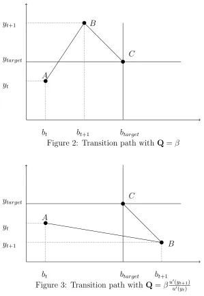
Precau-C B
A ytarget
btarget yt
bt yt+1
[image:17.612.140.439.67.500.2]bt+1
Figure 2: Transition path with Q=β
C
B A
ytarget
btarget yt
bt yt+1
bt+1
Figure 3: Transition path with Q=βu′(yt+1)
u′(yt)
tionary Principle. However, equation (7) implies that the use of a time constant discount
rate would lead to a situation where an increase in harvesting is the optimal response to a
0.5 1 1.5
SSB
t
0.8 0.85 0.9 0.95 1 1.05 1.1 1.15 1.2
Ft
Constant Discount
0.5 1 1.5
SSB
t
0.8 0.85 0.9 0.95 1 1.05 1.1 1.15 1.2
Ft
Non Constant Discount
0.5 1 1.5
SSBt
0.8 0.85 0.9 0.95 1 1.05 1.1 1.15 1.2
Ft
Constant Discount
0.5 1 1.5
SSBt
0.8 0.85 0.9 0.95 1 1.05 1.1 1.15 1.2
Ft
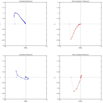
[image:18.612.143.472.147.477.2]Non constant Discount
Figure 4: Combinations of yield and SSB along optimal exploitation paths. The parame-terization for the age-structured population is the same as that shown in Da Rocha et al.
4
Conclusions
Fisheries management increasingly acknowledges that the variability in returns of a fishery
should be considered when seeking management strategies aimed at the MEY.5 In this
con-text, we investigate the implications of introducing invariant intertemporal preferences as to
yield stability in natural resource management problems where age-structured is crucial.
Intertemporal preferences as to yield stability are compromise approaches that allow
man-agement to adapt to natural fluctuations in stock abundance and reduce the uncertainty of
future fishing opportunities and the financial risk for fishermen, who depend on a stable
eco-nomic return over time. Moreover, when there is low yield variability in fisheries there is also
a more stable food supply, which prevents market saturation or price spikes, and contributes
to food security. These are common features shared with agriculture food production, also
characterised by high financial risk as a result of high year-to-year variation particularly for
farmers in developing countries, and by the economic importance of having reliable food
pro-duction (see e.g. Kasperski and Holland, 2013; Deepak et al.,2015). In forestry, continuous
cover forestry projects are attracting increasing interest as alternatives to rotation systems
of forest management (see e.g. Pukkala et al., 2010; Price and Price, 2006;Tahvonen, 2015)
in order to best combine timber production with other multiple benefits, where it is not only
the timber stock in a long term objective that is important but also the impact that tree
harvesting has on the maintenance of other benefits (recreational, biodiversity, non-timber
products, carbon storage, etc) (see e.g. Touza et al., 2008; Goetz et al., 2010; Kuuluvainen
et al., 2012).
Our results analytically show that in an age-structured model with a CES utility function,
if some proportionality is to be maintained between growth rates of annual catches and the
age-structure equivalent to biomass (i.e. the changes in the age-diversity of the population
5For example, Current fishery regulations often include a cap on interannual TAC variations (e.g.Kell
with respect to the steady-state target), then the discount rate should be non constant. We
can therefore conclude that preferences over time expressed as to the discounting process
are key in managing age-structured resources. Constant discounting would not guarantee
proportional growth rates, and would also have implications for the transition of the resource
towards the steady state. The use of a time-constant discount rate would lead to a situation
where an increase in harvesting was the optimal response to a fall in biomass levels. Such
a policy goes against the precautionary principle followed by most fisheries agencies, where
the desirability of implementing alternative harvesting control rules is explored in line with
their ability to steer toward an optimal exploitation level, stabilizing catches and driving
References
Aanesen, M., Armstrong, C., Bloomfield, H. J., and C., R. (2014). What does stakeholder
involvement mean for fisheries management? Ecology and Society, 19(4):35.
Baudron, A., Ulrich, C., Nielsen, J. R., and Boje, J. (2010). Comparative evaluation of
a mixed-fisheries effort-management system based on the faroe islands example. ICES
Journal of Marine Science, 67(5):1036–1050.
Da Rocha, J. M., Garcia-Cutrin, J., Gutierrez, M. J., and Touza, J. (2016). Reconciling
yield stability with international fisheries agencies precautionary preferences: the role of
non constant discount factors in age structured models. Fisheries Research, 173:282–293.
Da Rocha, J. M., Gutierrez, M. J., and Antelo, L. T. (2012). Pulse vs optimal stationary
fishing: The northern stock of hake. Fisheries Research, 121-122:51–62.
Da Rocha, J. M., Gutierrez, M. J., and Antelo, L. T. (2013). Selectivity, pulse fishing
and endogenous lifespan in Beverton-Holt models. Environmental Resource Economics,
54(1):139–154.
Deepak, K. R., Gerber James, S., MacDonald, G. K., and West, P. C. (2015). Climate
variation explains a third of global crop yield variability. Nature Communications, 6:5989.
Dichmont, C. M., Pascoe, S. K., Punt, T., E., A., and Deng, R. (2010). On implementing
maximum economic yield in commercial fisheries. Proceedings of the National Academy of
Sciences, 107(1):16–21.
Goetz, R., Hritonenko, N., Mur, R., Xabadia, A., and Yatsenko, Y. (2010). Forest
manage-ment and carbon sequestration in size-structured forests: the case of pinus sylvestris in
spain. Forest Science, 56:242 256.
asymmetric spatial dynamics on regulatory performance in a fishery metapopulation.
Eco-logical Economics, 77(C):207–218.
Kasperski, S. and Holland, D. S. (2013). Income diversification and risk for fishermen.
Proceedings of the National Academy of Sciences, 110(6):2076–2081.
Kell, L., Pilling, G., Kirkwood, G., Pastoors, M., Mesnil, B., Korsbrekke, K., Abaunza, P.,
Aps, R., Biseau, A., Kunzlik, P., Needle, C., Roel, B., and Ulrich, C. (2006). An evaluation
of multi-annual management strategies for ices roundfish stocks. ICES Journal of Marine
Science: Journal du Conseil, 63(1):12–24.
Kronbak, L. and Vestergaard, N. (2013). Environmental cost-effectiveness analysis in
in-tertemporal natural resource policy: evaluation of selective fishing gear. Journal of
Envi-ronmental Management, 131:270–279.
Kuuluvainen, T., Tahvonen, O., and Aakala, T. (2012). Even-aged and uneven-aged forest
management in boreal fennoscandia: a review. Ambio, 41(7):720–737.
Lassen, H. and Medley, P. (2000). Virtual population analysis. A Practical Manual for Stock
Assessment. FAO Fisheries Technical Paper, 400.
McGough, B., Plantinga, J. A., and Costello, C. (2009). Optimally managing a stochastic
renewable resource under general economic conditions. The B.E. Journal of Economic
Analysis and Policy, 9(1):1–31.
Pascoe, S., Proctor, W., Wilcox, C., Innes, J., Rochester, W., and Dowling, N. (2009).
Stakeholder objective preferences in australian commonwealth managed fisheries. Marine
Policy, 33(5):750–758.
Penas, E. (2007). The fishery conservation policy of the European Union after 2002: towards
Price, M. and Price, C. (2006). Creaming the best, or creatively transforming? might felling
the biggest trees first be a win-win strategy.Forest Ecology and Management, 224:297–303.
Pukkala, T., L¨ahde, E., and Laiho, S. (2010). Optimizing the structure and management of
uneven-sized stands of finland. Forestry, 84:129–142.
Quaas, M. F. and Requate, T. (2013). Sushi or fish fingers? seafood diversity, collapsing fish
stocks, and multispecies fishery management. The Scandinavian Journal of Economics,
115(2):381–422.
Ravn-Jonsen, L. (2011). Intertemporal choice of marine ecosystem exploitation. Ecological
Economics, 70:1726–1734.
Sampedro, P., Prellezo, R., Garc´ıa, D., Da Rocha, J. M., Cervi˜no, S., Torralba, J., Touza,
J., Garc´ıa-Cutr´ın, J., and Gutierrez, M. J. (2016). To shape or to be shaped: engaging
stakeholders in fishery management advice. ICES Journal of Marine Science, In Press.
Tahvonen, O. (2009). Economics of harvesting age-structured fish populations. Journal of
Environmental Economics and Management, 58(3):281–299.
Tahvonen, O. (2015). Economics of naturally regenerating, heterogeneous forests. Journal
of the Association of Environmental and Resource Economists, 2(2):309–337.
Touza, J., Termansen, M., and Perrings, C. (2008). A bioeconomic approach to the
faustmann-hartman rule: ecological interactions and even-aged forest management.
Nat-ural Resource Modeling, 21(4):551– 581.
Woods, P., Bourchard, C., Holland, D., Punt, A., and Marteinsdottir, G. (2015).
Catch-quota balancing mechanisms in the icelandic multi-species demersal fishery: are all species
A
Appendix
A.1
Log-linearizing yield over cycles
Log-linearization explores the trajectories in the proximity of the stationary solution in section 3.1,
with equation (2) being written as follows:
U′
(Y(N1, N2, N1′, N ′
2)) =−β2Hi(N1, N2, N1′, N ′ 2),
where
Hi(N1, N2, N1′, N
′ 2) =
∂V(N′
1,N2′)
∂N′
i
∂Y(N1,N2,N1′,N2′)
∂N′
i
i= 1,2.
By log-linearizing Hi(n1, n2, n′1, n ′
2) around Hi(N1, N2, N1′, N ′
2), where n1, n2, n′1, n ′
2 represent
states of the juvenile and adult population in periodst y t+ 2 in the proximity of the stationary
solution, we obtain,
Hi(n1, n2, n′1, n
′
2) − Hi(N1, N2, N1′, N ′ 2) = 2 X j=1
(∂Hi(N1, N2, N
′ 1, N
′ 2)
∂Nj
Nj)
| {z }
Bi,j
(lnnj−lnNj)
+
2
X
j=1
(∂Hi(N1, N2, N
′ 1, N
′ 2) ∂N′ j N′ j)
| {z }
Ai,j
(lnn′
j−lnNj),
where
Bi,j =−Hi(N1, N2, N1′, N
′ 2)
∂2Y(N
1,N2,N1′,N2′)
∂Nj∂Ni′
∂Y(N1,N2,N1′,N2′)
∂N′
i
Nj
Ai,j =Hi(N1, N2, N1′, N
′ 2)
∂2V(N′
1, N ′ 2)/∂N
′
j∂N
′
i
∂V(N′
1, N ′ 2)/∂N
′
i
−
∂2Y(N
1,N2,N1′,N2′)
∂N′
j∂Ni′
∂Y(N1,N2,N1′,N2′)
Given that in a stationary solution N′
j = Nj, ∆Hi =Hi(n1, n2, n′1, n ′
2)−Hi(N1, N2, N1′, N ′ 2) can
be expressed as
∆Hi =Ai,1ln(
n′
1
N1
) +Ai,2ln(
n′
2
N2
) +Bi,1ln(
n1
N1
) +Bi,2ln(
n2
N2
).
If we denote
εpi,j = ∂
2V(N′ 1, N
′ 2)/∂N
′
j∂N
′
i
∂V(N′
1, N ′ 2)/∂N
′
i
Nj,
εNj =
∂2Y
(N1,N2,N1′,N2′)
∂Nj∂Ni′
∂Y(N1,N2,N1′,N2′)
∂N′
i
Nj,
εN′
j =
∂2Y(N
1,N2,N1′,N2′)
∂N′
j∂Ni′
∂Y(N1,N2,N1′,N2′)
∂N′
i
Nj,
and log-linearize the left-hand term of the f.o.c. as given in equation (A.1) yields equation (3)
U′′
(Yss)Yss
U′(
Yss) ln(
Yt Yss ) = 2 X j=1
(εpi,j−εN′
j) ln(
n′ j Nj )− 2 X j=1
εNjln(
nj
Nj
).
A.2
Proof of Proposition
1
Log-linearizingHi(n1, n2, n′1, n ′
2, yt, yt+1) aroundHi(N1, N2, N1′, N ′
2), wheren1,n2,n′1,n ′
2, as above,
represent states of the juvenile and adult population in periods t y t+ 2 in the proximity of the
steady state, yields,
Hi(n1, n2, n′1, n
′
2, yt, yt+1) − Hi(N1, N2, N1′, N ′ 2) = 2 X j=1
(∂Hi(n1, n2, n
′ 1, n
′
2, yt, yt+1)
∂Nj
Nj)
| {z }
Bi,j
(lnnj−lnNj)
+
2
X
j=1
(∂Hi(n1, n2, n
′ 1, n
′
2, yt, yt+1)
∂N′
j
N′
j)
| {z }
Ai,j
(lnn′
j−lnNj)
+
1
X
j=0
(∂Hi(n1, n2, n
′ 1, n
′
2, yt, yt+1)
∂yt+j
yss)
| {z }
Ci,j
and
u′′
(yss)yss
u′(y
ss)
ln( yt
yss
) − (Ci,1lnyt+1+Ci,0lnyt) + (Ci,1+Ci,0)) lnyss
=
2
X
j=1
(εpi,j−εN′
j) ln(
n′
j
Nj
)−
2
X
j=1
εNjln(
nj
Nj
).
When u(y) = 1−1σy1
−σ, and given that (in steady stateC
i,0=−Ci,1), we have
σln( yt
yss
)−Ci,1ln(
yt+1
yt
) =
2
X
j=1
(εpi,j−εN′
j) ln(
n′
j
Nj
)−
2
X
j=1
εNjln(
nj
Nj
).