Looking for efficient qml estimation of conditional value at risk at multiple risk levels

Munich Personal RePEc Archive

Looking for efficient qml estimation of

conditional value-at-risk at multiple risk

levels

Francq, Christian and Zakoian, Jean-Michel

CREST, Université Lille 3

October 2015

Online at

https://mpra.ub.uni-muenchen.de/67195/

Looking for efficient QML estimation of conditional VaRs at

multiple risk levels

Christian Francq∗_{and Jean-Michel Zakoïan}†

Abstract

We consider joint estimation of conditional Value-at-Risk (VaR) at several levels, in the framework of general GARCH-type models. The conditional VaR at level α is expressed as the product of the volatility and the opposite of the α-quantile of the innovation. A standard method is to estimate the volatility parameter by Gaussian Quasi-Maximum Likelihood (QML) in a first step, and to use the residuals for estimating the innovations quantiles in a second step. We argue that the Gaussian QML may be inefficient with respect to more general QML and can even be in failure for heavy tailed conditional distributions. We therefore study, for a vector of risk levels, a two-step procedure based on a generalized QML. For a portfolio of VaR’s at different levels, confidence intervals accounting for both market and estimation risks are deduced. An empirical study based on stock indices illustrates the theoretical results.

JEL Classification: C13, C22 and C58.

Keywords: Asymmetric Power GARCH, Distortion Risk Measures, Estimation risk, Non-Gaussian Quasi-Maximum Likelihood, Value-at-Risk.

1

Introduction

In July 2009, the Basel Committee issued a directive requiring that financial institutions quantify

"model risk". The Committee states that "Banks must explicitly assess the need for valuation

ad-justments to reflect two forms of model risk: the model risk associated with using a possibly incorrect

valuation methodology; and the risk associated with using unobservable (and possibly incorrect)

cal-ibration parameters in the valuation model." For instance, an important issue in determining the reserves of a financial institution is whether risk estimates remain reliable in very turbulent periods.

To this aim, the recent econometric literature on risk has focused on the concept of estimation risk. Whatever the risk measure, it depends on unknown characteristics of the loss distribution

∗_{CREST and University Lille 3, BP 60149, 59653 Villeneuve d’Ascq cedex, France. E-Mail:}

[email protected]

†_{Corresponding author: Jean-Michel Zakoïan, University Lille 3 and CREST, 15 boulevard Gabriel Péri, 92245}

which, for practical use, have to be estimated. For instance, the Value-at-Risk (VaR) at a given

level α, can be defined as the opposite of the α-quantile of the loss distribution. In advanced approaches of risk measurement, the statistical framework is complicated by the dynamic nature of the loss variables. The corresponding risk measures have to be considered conditional on the past

losses, and are therefore called conditional risk measures.

In recent research, different approaches were proposed to account for the presence of estimation

risk in conditional risk measurement. Chan, Deng, Peng, Xia (2007) constructed confidence intervals

for conditional VaRs under the assumption that the errors have heavy tails, using the Extreme-Value Theory, while Spierdijk (2013) proposed a residual subsample bootstrap approach. A bootstrap

testing procedure, for the equality of conditional VaRs in a multivariate setting, was recently studied by Hurlin, Laurent, Quaedvlieg and Smeekes (2013). Francq and Zakoïan (2015) showed that the problem of estimating a conditional risk measure, for instance a VaR at a given level, in

GARCH-type models reduced to the estimation of a parameter, called risk parameter. They derive an asymptotic theory for a Gaussian Quasi-Maximum Likelihood (QML) of this parameter. For the

same problem, a more general approach based on non-Gaussian QMLs was studied by El Ghourabi, Francq and Telmoudi (2015). Gouriéroux and Zakoïan (2013) investigated the bias induced by

estimation in the coverage probabilities associated with VaR. Escanciano and Olmo (2010) studied the effect of estimation on backtesting VaR.

In the inference of GARCH-type models, recent articles underlined the possible efficiency loss of the QML estimator (QMLE) due the use of an inappropriate Gaussian error distribution (see Berkes

and Horváth (2004), Francq, Lepage and Zakoïan (2011), Francq and Zakoïan (2013), Fan, Qi and Xiu (2014)). In the present paper, we study the estimation of a vector of conditional VaRs based on

generalized QMLEs of the volatility. We extend the article by Francq and Zakoïan (2014) devoted to the Gaussian QML by considering QML criteria based on "instrumental densities" which, in general,

will not coincide with the errors distribution. We consider a general GARCH-type framework which does not impose a specific form for the volatility. Our approach is aimed at, not only providing VaR

estimates, but also confidence intervals based on asymptotic results. The introduction of several risk levels provides a better account of the tail properties of the conditional loss distribution. The VaRs

is the main aim of the paper. We also show how efficiency gains can be reached by selecting an

appropriate instrumental density.

This paper is structured as follows. In Section 2, we derive the asymptotic joint distribution of the generalized QMLE of the volatility parameter, and a vector of empirical quantiles of the

residuals. In Section 3, we deduce asymptotic confidence intervals for the VaR portfolios. The choice of an optimal criterion is also discussed. An empirical illustration based on major stock

indices is proposed in Section 4. Section 5 concludes.

2

Non-Gaussian QMLE of vectors of VaRs

2.1 Conditional VaR in a general model

GARCH-type models are arguably the most widely used discrete-time volatility models. Most of them can be written under the form

  

ǫt=σtηt

σt=σ(ǫt−1, ǫt−2, . . .;θ0)

(2.1)

where (ηt) is a sequence of iid random variables, ηt is independent of {ǫu, u < t}, θ0 ∈ Rd is a

parameter belonging to a parameter space Θ_{, and σ : R}∞_×Θ_{→(0,∞). A standard assumption}

is thatEη_t2 = 1but, unless otherwise stated, we do not make this assumption in the present article. An example of widely used specification is the Asymmetric Power GARCH (APARCH) model

introduced by Ding, Granger and Engle (1993). Letting x+= max(x,0) andx−= max(−x,0), the APARCH(p, q) model is defined by

  

ǫt=σtηt

σ_tδ=ω0+Pqi=1

α0i+(ǫ+t−i)δ+α0i−(ǫ−t−i)δ +

Pp

j=1β0jσδt−j

(2.2)

where the coefficients satisfyα0i+ ≥0,α0i−≥0,β0j ≥0,ω0>0andδ >0. The standard GARCH

model is obtained forδ= 2andα0i− =α0i+. Whenα0i−> α0i+, negative returns have more impact

on future volatilities than positive returns of the same magnitude, which is the well-documented

"leverage effect".

The conditionalVaR of a process (ǫt) at risk levelα∈(0,1), denoted by VaRt(α), is defined by

where Pt−1 denotes the historical distribution conditional on{ǫu, u < t}. When (ǫt) satisfies (2.1),

the conditional VaR is then given by

VaRt(α) =−σ(ǫt−1, ǫt−2, . . .;θ0)ξα (2.3)

where ξα is theα-quantile of ηt.

Remark 2.1 It can be noted that in the PARCH(p, q) model, the conditional VaR at level α

satisfies the stochastic recurrence equation

VaRδ_t(α) = ω0(−ξα)δ+ q

X

i=1

n

α0i+(ǫ+_t−i)δ+α0i−(ǫ−_t−i)δ

o

(−ξα)δ

+

p

X

j=1

β0jVaRδt−j(α). (2.4)

Direct modelling of the conditional VaR has been proposed in several papers, for instance Engle and Manganelli (2004), Koenker and Xiao (2006), Gouriéroux and Jasiak (2008). A difficulty with

conditional VaR dynamic models is to constrain the model so as to guarantee the monotonicity of the conditional VaR as a function of the risk level. Monotonicity is automatically satisfied in (2.4).

It will be convenient to assume that the parametric form of the volatility is stable by scaling.

A0: There exists a continuous function H such that for any θ _∈ Θ_{, for any K > 0, and any}

sequence(xi)i

Kσ(x1, x2, . . .;θ) =σ(x1, x2, . . .;H(θ, K)).

This assumption is clearly satisfied for all commonly used GARCH models (see Section 2.3 for the

APARCH model).

When ξα<0,A0 and (2.3) entail

VaRt(α) =σ(ǫt−1, ǫt−2, . . .;θ(0α)), θ (α)

0 =H(θ0,−ξα). (2.5)

This parameterθ(₀α), introduced by Francq and Zakoïan (2015) for more general risk measures, can

2.2 Asymptotic properties of a vector of conditional VaR estimators

A two-step standard method for evaluating the VaR at different levels αi ∈(0,1), for i= 1, . . . , m

consists in estimating the volatility parameterθ₀ by Gaussian QMLE, and then estimating the ξαi

by the corresponding empirical quantiles of the residuals; see, for instance, Chapter 2 in McNeil,

Frey and Embrechts (2005). For a comparison of alternative strategies based on residuals following a preliminary volatility estimation, see Kuester, Mittnik and Paolella (2006). El Ghourabi, Francq

and Telmoudi (2015) showed that, in this two-step procedure, the Gaussian QML can be replaced by any non-Gaussian QML. We now extend this approach to a vector of VaRs at different risk levels.

Given observations ǫ1, . . . , ǫn, and arbitrary initial valueseǫi for i≤0, we define

e

σt(θ) =σ(ǫt−1, . . . , ǫ1,eǫ0,eǫ−1, . . .;θ),

which is used to approximate σt(θ) =σ(ǫt−1, . . . , ǫ1, ǫ0, ǫ−1, . . .;θ).

Given an instrumental density h >0, consider the QML criterion

e

Qn(θ) =

1

n

n

X

t=1

g(ǫt,σet(θ)), g(x, σ) = log

1

σh

_x

σ

, (2.6)

and the (generalized) QMLE

ˆ

θn,h= arg max

θ∈ΘQen(θ). (2.7)

This estimator is the standard Gaussian QMLE if h is the standard Gaussian density φ. We emphasize that the parametric form ofσt(·)is assumed to be correctly specified, but we do not make

precise assumptions on the distribution of ηt. In particular, we do not assume that Var(ηt) = 1. 1

Consequently, bθ_n,hwill be a consistent estimator of some pseudo-value (to be defined below) θ_0,h. The following assumptions will be used to derive the asymptotic properties of the QMLE bθn,h.

A1: (ǫt) is a strictly stationary and ergodic solution of Model (2.1). Moreover, E|ǫ0|s < ∞ for

some s >0.

A2: Almost surely, σt(θ) ∈ (ω,∞] for any θ ∈ Θ and for some ω > 0. For θ1,θ2 ∈Θ, we have

σt(θ1) =σt(θ2)a.s.if and only if θ1 =θ2.

Note that

g(ǫt, σt(θ)) =g

ηt,

σt(θ)

σt(θ0)

−logσt(θ0). (2.8)

1

A3: The function σ _→ Eg(η0, σ) takes its values in [−∞,+∞) and has a unique maximum at

some pointσh∈(0,∞).

A4: The instrumental densityhis twice continuously differentiable onR, except possibly in 0, and there exist constants r≥0and C0>0such that, for all u∈R\ {0},

maxuh

′_(u)

h(u)

, u2

h′(u)

h(u)

′

≤C0(1 +|u|r), with E|η0|2r <∞.

A5: The functionθ_7→σ(x1, x2, . . .;θ) has continuous second-order derivatives, and

sup

θ∈Θ

|σt(θ)−σet(θ)|+

∂σt(θ)

∂θ −

∂_eσt(θ)

∂θ +

∂2σt(θ)

∂θ∂θ′ −

∂2_eσt(θ)

∂θ∂θ′

≤C1ρt,

where C1 is a random variable which is measurable with respect to {ǫu, u <0} andρ∈(0,1)

is a constant.

A6: θ0,h=H(θ0, σh) belongs to the interior ofΘ.

A7: There exist no non-zero x_∈Rdsuch that x′∂σt(θ0,h)

∂θ = 0, a.s.

A8: There exists a neighborhood V(θ_0,h) of θ_0,h such that the following variables have finite expectation:

sup

θ∈V(θ0,h)

1

σt(θ)

∂σt(θ)

∂θ 4 , sup

θ∈V(θ0,h)

1

σt(θ)

∂2_σ

t(θ)

∂θ∂θ′

2 , sup

θ∈V(θ0,h)

σt(θ0,h)

σt(θ)

2r .

Remark 2.2 AssumptionA3reduces toE|η0|r <∞, and AssumptionA4reduces toE|η0|2r<∞

for instrumental densities of the formh(u) =K1|u|λexp{K2|u|r}, for some constantsλ, K1, K2.

Remark 2.3 The numberσhinvolved in AssumptionA3depends on both the density ofηtand the

instrumental densityh. It can be made explicit for classes of densityh(see El Ghourabi, Francq and Telmoudi (2015)). For instance, whenh belongs to the class of the Generalized Error Distributions with shape parameter κ >0, defined by

hκ(x) =

κ

Γ(1/κ)21+1/κe

−|x2|κ,

we have

σhκ =

_κ

2E|η1|

Now letηt,h= _σ1_hηt and letξα,h= _σ1_hξα theα-quantile ofηt,h. Noting that

ǫt=σ(ǫt−1, ǫt−2, . . .;θ0)ηt=σ(ǫt−1, ǫt−2, . . .;θ0,h)ηt,h,

we have, by (2.5) andA3,

VaRt(α) =σ(ǫt−1, ǫt−2, . . .;θ(0α)), θ (α)

0 =H(θ0,−ξα) =H(θ0,h,−ξα,h). (2.9)

In view of the last equality, a strategy for consistently estimating θ(₀α) is thus to estimate θ_0,h by generalized QML in the first step, and to estimate the quantile ξα,h in the second step. Let the

residuals of the QML estimation

ˆ

ηt,h =

ǫt

e

σt(bθn,h)

, t= 1, . . . , n,

and let ξn,αi,h denote the empirical αi-quantile of ηˆ1,h, . . . ,ηˆn,h. Let α = (α1, . . . , αm)

′_{, ξ}

n,α_,h =

(ξn,α1,h, . . . , ξn,αm,h)

′ _{and letξ}

α,h= (ξα1,h, . . . , ξαm,h)

′ _{denote the vector of population quantiles.}

The next result gives the joint asymptotic distributions of (bθ′_n,h,ξ_n,′ α). Let Dt(θ) =

σ_t−1(θ)∂σ_∂t(_θθ), g1(x, σ) = ∂g(_∂σx,σ) and g2(x, σ) = ∂g1_∂σ(x,σ).

Theorem 2.1 Assume ξαi,h < 0, for i = 1, . . . , m. Suppose η0,h admits a density fh which is

continuous and strictly positive in a neighborhood ofξαi,h, fori= 1, . . . , m. Assume Eg2(η0,h,1)6=

0. Let A0-A8 hold, with r >1 in A4 and A8. Then

 

√

nbθn,h−θ0,h

√

n(ξ_n,α_,h−ξα_,h)



 _{→ N}L (0,Σ_α,h), Σ_α,h= 

 τhJ

−1

h λ′α_,h⊗J−_h1Ωh

λα_,h⊗Ω′_hJ−_h1 ζα_,h

 ,

where

τh=

4Eg2₁(η0,h,1)

{Eg2(η0,h,1)}2

, Ω_{h =EDt(θ0,h), Jh= 4EDt(θ0,h)D}′

t(θ0,h),

λα,h= (λα1,h, . . . , λαm,h)

′_,ζ

α_,h= (ζij,h)1≤i,j≤m and

λαi,h = −ξαi,hτh+

4pαi,h

fh(ξαi,h)Eg2(η0,h,1)

,

ζij,h = ξαi,hξαj,h

τh

4 −

1

Eg2(η0,h,1)

_ξ

αi,hpαj,h

fh(ξαj,h)

+ξαj,hpαi,h

fh(ξαi,h)

+ αi∧αj−αiαj

fh(ξαi,h)fh(ξαj,h)

,

withpα,h=Cov

n 1_{η

0,h<ξα,h}, g1(η0,h,1)

o

Proof. In view of El Ghourabi, Francq and Telmoudi (Proof of Theorem 1, 2015), we have, for

i= 1, . . . , m,

√

n(ξαi,h−ξn,αi,h) = ξαi,hΩ

′ h

√

n(θbn,h−θ0,h)

+ 1

fh(ξαi,h)

1 √ n n X t=1

(1_{η

t,h<ξ_αi,h}−αi) +oP(1),

and

√

n(bθn,h−θ0,h) = −

4

Eg2(η0,h,1)

J−_h1√1

n

n

X

t=1

g1(ηt,h,1)Dt(θ0,h) +oP(1).

Hence

Covas √n(bθn,h−θ0,h),

1 √ n n X t=1

(1_{η

t,h<ξ_αi,h}−αi)

!

= −4pαi,h

Eg2(η0,h,1)

J−_h1Ω_h.

It follows that, for i_≤j,

Covas{√n(ξαi,h−ξn,αi,h),

√

n(ξαj,h−ξn,αj,h)}

=

ξαi,hξαj,hτh−

4

Eg2(η0,h,1)

_ξ

αi,hpαj,h

fh(ξαj,h)

+ξαj,hpαi,h

fh(ξαi,h)

Ω′

hJ−h1Ωh

+ αi(1−αj)

fh(ξαi,h)fh(ξαj,h)

,

Covas

_√

n(bθn,h−θ0,h),√n(ξαi,h−ξn,αi,h)

= λαi,hJ

−1

h Ωh.

We have Ω′

hJ−h1Ωh= 1/4 (see Remark 3.1 in Francq and Zakoïan, 2013) and thus we obtain

Covas{√n(ξαi,h−ξn,αi,h),

√

n(ξαj,h−ξn,αj,h)} = ζij.

By the CLT for martingale differences, we get the announced result. ✷

LetVaRt(α) = (VaRt(α1), . . . ,VaRt(αm))′, the vector of conditional VaRs at levelsαi. In view

of

VaRt(α) =−σ(ǫt−1, ǫt−2, . . .;θ0,h)ξα,h, (2.10)

the vector of conditional VaRs can be estimated by

[

Remark 2.4 In classical quantile regression, a serious problem is that the estimated quantile curves can cross, leading to an invalid inference at multiple percentiles (see Koenker (2005)). It is thus worth noting that our estimation procedure does not face this problem. By construction, the estimated conditional VaR are monotonous functions of the α’s.

Remark 2.5 The coefficientτh can be made explicit for different classes of density functionsh. For

instance, for the GED distribution of Remark 2.3, simple computation shows that for the density

hκ,

τh=

4

κ2

E_|η1|2κ

(E|η1|κ)2

−1

!

.

In other cases, such as the class of the Student densities, coefficients τh and σh do not have an

explicit expression but can be obtained numerically.

Remark 2.6 It should be noted that the coefficient τh appearing in the asymptotic distribution

only depends on i) the distributional properties of the variable η0 and ii) the choice of the QML

density h. For a given h, the coefficient τh can be estimated using the residualsηˆt,h by

ˆ

τh = 4

n−1Pn_t=1g₁2(ˆηt,h,1)

{n−1Pn

t=1g2(ˆηt,h,1)}2

. (2.12)

The residualsηˆt,h can be used to estimate the density fh, as well as all other quantities involved in

the asymptotic distribution.

2.3 Application to the APARCH model

For the APARCH(p, q) model with δ fixed2, we have θ = (ω, α1+, . . . , αq−, β1, . . . , βp)′ and A0

is satisfied with H(θ, K) = (Kδω, Kδα1+, . . . , Kδαq−, β1, . . . , βp)′. The parameter is assumed to

belong to a compact set Θ _⊂]0,+_∞[_×[0,+_∞[p+2q. Let _Aθ+(z) = Pqi=1αi+zi and Aθ−(z) =

Pq

i=1αi−zi Bθ(z) = 1 −

Pp

j=1βjzj with, by convention, Aθ+(z) = Aθ−(z) = 0 if q = 0 and

Bθ(z) = 1 if p= 0. Let γ denote the Lyapunov coefficient of the sequence (At) associated with the

vector representation of the model. Hamadeh and Zakoïan (2011) showed the CAN of the Gaussian

QMLE of θ0 under the assumption:

2

Hamadeh and Zakoïan (2011) showed that estimating the powerδ is feasible though complicated. We therefore

considerδ as fixed. In most applications,δ is either equal to 1 (as in the TARCH of Zakoïan (1994)) or to 2 (as in

D(θ0): γ < 0; the true parameter value θ0 belongs to the interior of Θ; there exists ω > 0 such

that,∀θ_∈Θ_{, ω > ω and}Pp

j=1βj <1 ; the support of the distribution ofη0 contains at least

3 points;P[ηt>0]∈(0,1); ifp >0,Bθ0(z) has no common root withAθ0+(z) and Aθ0−(z);

Aθ0+(1) +Aθ0−(1)6= 0 and α0q,++α0q,−+β0p 6= 0

and under the identifiability condition Eη₁2 = 1(which we do not assume in our framework). For any θ _∈Θ_{, letθ}′ _{= (ω, α1+, . . . , αq−,0, . . . ,0). We have,}

θ′∂σ

δ t(θ)

∂θ = ω+

q

X

i=1

n

αi+(ǫ+t−i)δ+αi−(ǫ−t−i)δ

o

+

p

X

j=1

βjθ

′∂σδt−j(θ)

∂θ

= _Bθ−1(L) ω+

q

X

i=1

n

αi+(ǫ+t−i)δ+αi−(ǫ−t−i)δ

o!

=σδ_t(θ),

where L denotes the usual lag operator. Therefore,

θ′ 1

σt

∂σδ t(θ)

∂θ = 1

δ,

and thus

θ′_0,hΩ_{h =} 1

δ, J

−1

h Ωh =

δ

4θ0,h.

It follows that Theorem 2.1 can be simplified as follows in the case of the APARCH model.

Corollary 2.1 Consider the APARCH(p, q) model (2.2) under Assumption D(θ0,h). Assume

ξαi,h < 0, for i = 1, . . . , m. Suppose η0,h admits a density fh which is continuous and strictly

positive in a neighborhood of ξαi,h, fori= 1, . . . , m. If the instrumental densityh satisfies A3, A4,

and ifEg2(η0,h,1)6= 0, then

 

√

nbθn,h−θ0,h

√

n(ξ_n,α,h−ξα,h)

  L

→ N(0,Σα_,h), Σα_,h=



 τhJ

−1

h λ′α,h⊗4δθ0,h

λα,h⊗ δ₄θ ′

0,h ζα,h

 .

2.4 Optimal choice of the density h

El Ghourabi, Francq and Telmoudi (2015) showed that, for the VaR estimation at a single level, an optimal choice of the densityhis obtained by minimizing (within a class of densities) the coefficient

τh. For such an optimal density h∗, the accuracy of the VaR estimation is maximal. Interestingly,

For instance, when the density h is chosen among the GED densities, in view of Remark 2.5 an optimal value for κcan be estimated by taking

ˆ

κ= arg min

κ∈K

1

κ2

_µˆ

2κ

ˆ

µ2

κ −

1

, µˆr=

1

n

n

X

t=1

|ηˆt,h|r, (2.13)

for some compact set K ⊂R+_{.Practical implementation, for any given classH of densitiesh, thus}

involves the following steps:

1. For any h0 ∈ H, compute θˆn,h0 by solving (2.7) (forh=h0).

2. Using the residuals ηˆt,h0 of the first step, compute the coefficients

ˆ

τh= 4

n−1Pn_t=1g2₁(ˆηt,h0,1)

{n−1Pn

t=1g2(ˆηt,h0,1)}

2, (2.14)

where g1, g2 are defined before Theorem 2.1. Solveh∗ = arg maxh∈Hτˆh.

3. Computeθˆ_n,h∗ and deduce the conditional VaR from (2.11) (with h∗ instead of h).

3

Portfolios of VaR’s

Risk measurement based on a single VaR at a given level can be misleading since it gives a limited view of the loss distribution. To circumvent this problem, DRMs have been introduced in the insurance literature, in a series of papers by Wang and coauthors [see Wang (2000) and the references

therein]. General conditional DRMs take the form

DRMt=

Z 1

0

VaRt(u)dG(u), (3.1)

where the distortion function,G, is a given cumulative distribution function (cdf) on[0,1]. It follows from (2.3) that, for Model (2.1),

DRMt=−σ(ǫt−1, ǫt−2, . . .;θ0)

Z 1

0

ξudG(u). (3.2)

3.1 Estimating the discrete DRM parameter

If−R₀1ξudG(u)>0, the DRM in (3.2) can be written as

where θG₀ defined by

θG₀ =H

θ0,−

Z 1

0

ξudG(u)

(3.4)

is called DRM-parameter (similarly to the VaR parameter in (2.5)).

In the spirit of DRM, a risque measure which can be interpreted as a portfolio of VaR’s at

different levels is defined by

p′VaRt(α) = m

X

i=1

piVaRt(αi), (3.5)

where p = (p1, . . . , pm) with pi ≥ 0 for i = 1, . . . , m and Pmi=1pi = 1. This risk measure can be

interpreted as adiscrete DRMwith associated distortion function corresponding to Dirac masses at the points αi. By (2.3) we have

p′VaRt(α) = −σ(ǫt−1, ǫt−2, . . .;θ0)

m

X

i=1

piξα

= σ(ǫt−1, ǫt−2, . . .;θDRM0 ), where θDRM0 =H θ0,−p′ξα

(3.6)

can be calleddiscrete DRM-parameter. In view of (2.9), we also have, for any instrumental density

h,

θDRM₀ =H θ_0,h,−p′ξ_α,h,

from which we deduce an estimator of the discrete DRM-parameter given by

b

θDRM_n,h =Hbθn,h,−p′ξn,α,h

,

whose asymptotic distribution is a straightforward consequence of Theorem 2.1. Denoting by(θ, x) the generic arguments of the function H, let the d_×dmatrix A0,h = ∂H_∂θ′ θ0,h,−p

′_ξ α,h

and the

d×1 vector b_0,h= ∂H_∂x θ_0,h,−p′ξ_α,h.

Corollary 3.1 Under the assumptions of Theorem 2.1,

√

nbθDRM_{n,h −}θDRM_{0,h → N}L (0,ΣDRM_{α,h ),}

ΣDRM_{α,h = [A0,h −b0,hp}′_]Σ_α,h   A

′

0,h

−pb′_0,h

 .

Proof. We have, by a Taylor expansion of the function H(θ, x)around (θ_0,h,−p′ξ_α,h),

√

and the conclusion follows. ✷

It follows from (3.6) that the discrete DRM can be estimated by

p′VaR[t(α) = σet(θb DRM n,h ).

3.2 Constructing confidence intervals for the portfolio of VaR’s

LetΣb_{α,h denote a consistent estimator of the asymptotic variance} Σ_{α,h. Such an estimator can be}

constructed by i) replacing Jh by Jbn,h =n−1Pnt=1Dt(bθn,h)Dt(bθn,h)′; ii) using the residuals bηt,h

to construct an estimator fbh of the density function fh of the innovation ηt,h, and to replace the

theoretical moments of the process (ηt,h)by their empirical counterpart.

Let also Ab_n,h= ∂H_∂θ′

b

θ_n,h,−p′ξ_n,α,h,bb_n,h= ∂H_∂x bθ_n,h,−p′ξ_n,α,h and let

b

ΣDRM_{n,α,h = [A}b_{n,h −}b_bn,hp′_]Σb_n,α_,h

  Ab

′ n,h

−pbb′_n,h

 .

Corollary 3.1 and the delta method thus suggests a (1 ₋α0)% confidence interval (CI) for

p′VaRt(α)whose bounds are

p′VaR[t(α)±

Φ−_1−α1 _0/2

√

n

∂_eσt

∂θ′(bθ

DRM n,h )Σb

DRM

α,h

∂σ_et

∂θ (bθ

DRM n,h )

1/2

, (3.7)

where Φ−_α01 denotes the α0-quantile of the standard Gaussian distribution. It should be noted α0 (the risk estimation level) can be chosen independently from the αi’s (the financial risk levels).

Drawing such CIs allows to underline the importance of the estimation risk for VaR evaluation. In particular, a (1₋α0)%confidence interval (CI) for theVaRt(αi) is given by

−eσt(bθn,h)ξn,αi±

Φ−_1−α1

0/2

√

n

n b

∆_t,α,hΣb_α,h∆b′

t,α_,h

ii

o1/2

,

where

b

∆_t,α_,h = ξ_n,α,h

∂σ_et(θbn,h)

∂θ′ ,eσt(bθn,h)Im

!

, (3.8)

where Im denotes the m×m identity matrix

3.3 On the moment assumptions

important to note that the moments assumptions on the iid process required for the validity of the

asymptotic results depend on the choice ofh. Such moments assumptions appear in Assumptions A3 andA4 through the conditions

Eg(η0, σ)<∞ and E|η0|2r<∞,

where ther >0is determined, in the first part of A4, by the choice ofh.

To be more specific, consider instrumental densities of the formh(u) =K1|u|λexp{K2|u|r}, for

some constants λ, K1, K2. By Remark 2.2, the moment assumptions reduce to E|η0|2r <∞.

For instance, consider the usual Gaussian QMLE (r= 2andλ= 0). IfE_|η0|4 <∞, the two-step

VaR and discrete DRM parameter estimators are consistent and asymptotically normal. In view of Corollary 3.1, valid confidence intervals for the portfolio of VaR’s can be constructed. Now suppose

thatE|η0|2 = 1butE|η0|4 =∞. Then, under appropriate assumptions, the Gaussian QMLE of the

volatility parameter is well known to be consistent, and it could probably be established that the

discrete DRM parameter is also consistent. Hall and Yao (2003) derived a non standard asymptotic distribution for the estimator of the volatility parameter. However, establishing the analogous of

Theorem 2.1 in this situation would a formidable task. Finally, ifE|η0|2 =∞, the Gaussian QML

estimator of the volatility parameter is probably not even consistent.

If, instead, an instrumental density of the form h(u) = K1|u|λexp{K2|u|r} with r < 2 such

that E_|η0|2r < ∞ is chosen, then the estimator of the discrete DRM parameter has a standard

asymptotic distribution given by Corollary 3.1. In particular, our theory allows to handle GARCH models with Lévy alpha-stable conditional distributions.

To conclude this section, it is worth noting that estimating a portfolio of VaRs with a non-Gaussian instrumental density is not more demanding, in terms of computational burden, than

with the usual QMLE.

4

Empirical illustration

We now illustrate our theoretical results by considering a set of daily returns of 9 world stock

market indices: CAC (Paris), DAX (Frankfurt), FTSE (London), Nikkei (Tokyo), NSE (Bombay), SMI (Switzerland), SP500 (New York), SPTSX (Toronto), and SSE (Shanghai), collected from early

We compared two estimators of the discrete DRM (3.5), in which the m levels are equally spaced fromα1= 0.01 to αm= 0.10, and the weights are defined, for some r >0, by

p1=

αr

1

αr m

, pi=

αr

i −αri−1

αr m

, i= 2, . . . , m.

Note that the weights are derived from the so-called "proportional hazard" DRM. In particular

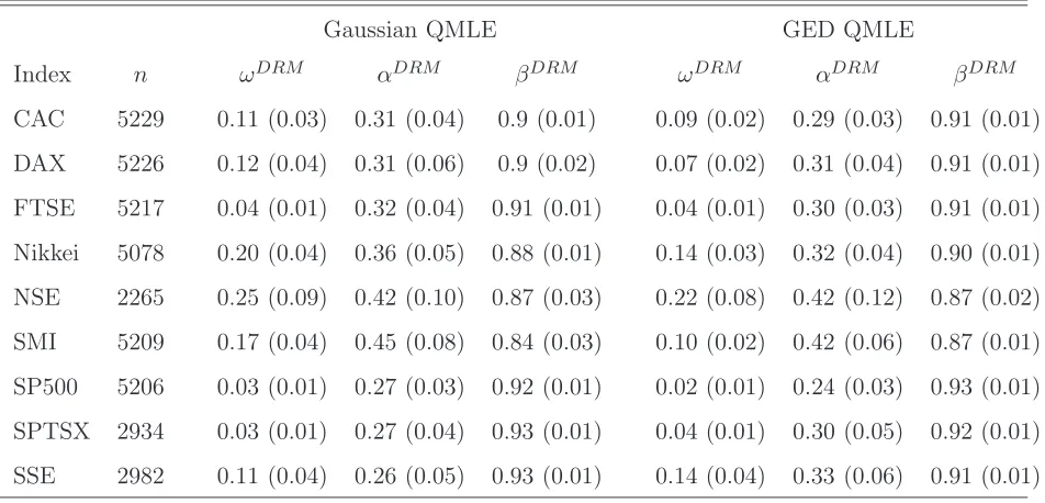
the weights decrease with i when r < 1 (which reflects risk aversion). The results presented in Table 1 correspond to r = 1/2 and m = 5, but the outputs are qualitatively similar for other choices of these coefficients. For the volatility specification we used a standard GARCH(1,1). The estimator displayed in the columns "Gaussian QMLE" is simply obtained with the usual Gaussian

instrumental density h = φ. For the estimator displayed in the columns "GED QMLE", we used an instrumental density within the GED(κ) class. We applied the three steps of Section 2.4 using the Gaussian QML in the first step.

Table 1 shows that the estimates of the DRM parameters produced by the two methods are

sim-ilar, with non empty intersections for confidence bounds whose widths are two estimated standard deviations. The estimated standard deviations are however systematically larger with the method

based on the Gaussian QMLE than with that based on the optimal GED instrumental density, which leads us to think that the second method is preferable.

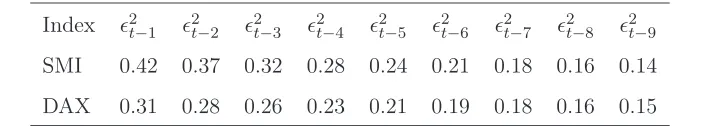
Although the estimated VaR parameters appear similar for all indices, some differences can be underlined. For instance, let us compare the VaR parameters estimated by the GED QML for the

DAX and the SMI. By (3.6), the conditional risk of the portfolio, p′VaRt(α) is estimated by

e

σt(bθ DRM

n,h ) = b

ωn

1₋βbn

+

t−1

X

i=1

b

αnβbniǫ2t−i,

!1/2

, (4.1)

where bθDRM_n,h = (_bωn,αbn,βbn)′. It is seen from Table 2 that the effect of a shock at time t−1 on

the estimated VaR of the portfolio will be much larger for the SMI than for the DAX. At longer horizons, however, the effects are reversed. It is worthnoting that this kind of interpretation is made

possible by the notion of VaR parameter, which jointly incorporates the effects of volatility and the tails of the conditional distribution.

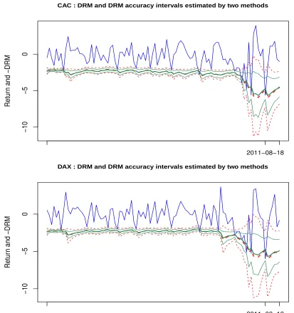
Figure 1 displays, for the CAC and DAX indices, the conditional DRM and its estimated 95%

Table 1: Estimation of the conditional discrete DRM parameter for 9 stock market indices. The estimated standard deviations are displayed into brackets.

Gaussian QMLE GED QMLE

Index n ωDRM αDRM βDRM ωDRM αDRM βDRM

CAC 5229 0.11 (0.03) 0.31 (0.04) 0.9 (0.01) 0.09 (0.02) 0.29 (0.03) 0.91 (0.01) DAX 5226 0.12 (0.04) 0.31 (0.06) 0.9 (0.02) 0.07 (0.02) 0.31 (0.04) 0.91 (0.01) FTSE 5217 0.04 (0.01) 0.32 (0.04) 0.91 (0.01) 0.04 (0.01) 0.30 (0.03) 0.91 (0.01)

Nikkei 5078 0.20 (0.04) 0.36 (0.05) 0.88 (0.01) 0.14 (0.03) 0.32 (0.04) 0.90 (0.01) NSE 2265 0.25 (0.09) 0.42 (0.10) 0.87 (0.03) 0.22 (0.08) 0.42 (0.12) 0.87 (0.02)

SMI 5209 0.17 (0.04) 0.45 (0.08) 0.84 (0.03) 0.10 (0.02) 0.42 (0.06) 0.87 (0.01) SP500 5206 0.03 (0.01) 0.27 (0.03) 0.92 (0.01) 0.02 (0.01) 0.24 (0.03) 0.93 (0.01)

SPTSX 2934 0.03 (0.01) 0.27 (0.04) 0.93 (0.01) 0.04 (0.01) 0.30 (0.05) 0.92 (0.01) SSE 2982 0.11 (0.04) 0.26 (0.05) 0.93 (0.01) 0.14 (0.04) 0.33 (0.06) 0.91 (0.01)

8, 2011 to August, 26, 2011 for the DAX index. The estimation of the DRM parameters is based

on the 1000 previous values. It can be seen that the estimated DRM’s are very close, but the CI’s

can be quite different. This is not surprising because we know from the asymptotic theory that the two methods are consistent, but that the method based on the optimal GED can be more efficient than that based on the Gaussian instrumental density (with corresponds to the particular GED

of parameter τ = 2). The difference is particularly important during turbulent periods (near the August 2011 stock markets fall).

It can be noted that in turbulent periods, both the market risk and the estimation risk increase. This is due to the fact that, as can be seen from (3.8), the derivatives of the VaR, with respect to

θ and to the quantiles of the innovations, increase with volatility. Participants of financial markets are well aware that the reserves should be increased in turbulent periods, but our conclusion is that

CAC : DRM and DRM accuracy intervals estimated by two methods

Retur

n and −DRM

−10

−5

0

2011−08−18

DAX : DRM and DRM accuracy intervals estimated by two methods

Retur

n and −DRM

−10

−5

0

2011−08−18

Figure 1: Returns (in blue) and (opposite of the) estimated discrete DRM and its 95% CI, with the Gaussian

Table 2: Coefficients of theǫ2

t−i in the estimated discrete DRM displayed in (4.1), for two indices.

Index ǫ2_t−1 ǫ2_t−2 ǫ2_t−3 ǫ2_t−4 ǫ2_t−5 ǫ2_t−6 ǫ2_t−7 ǫ2_t−8 ǫ2_t−9

SMI 0.42 0.37 0.32 0.28 0.24 0.21 0.18 0.16 0.14 DAX 0.31 0.28 0.26 0.23 0.21 0.19 0.18 0.16 0.15

5

Conclusion

In this paper, we considered the joint estimation of conditional VaRs at different levels, in the framework of conditionally heteroskedastic models. By considering a QML approach, we avoided

strong distributional assumptions on the noise sequence. The asymptotic results were established for a general class of QMLEs, including the usual Gaussian QMLE. The generalized QMLE converges to a volatility parameter which is specific to the chosen instrumental densityh. The true conditional VaR is obviously independent of the chosen parameterization and, interestingly, it can be estimated by any QML contrary to the volatility parameter. The VaR estimator and its asymptotic accuracy

depend on the specific QML, however. We showed how the choice ofh can be optimized, based on a preliminary QML estimation of the model, to gain in asymptotic accuracy.

We also introduced discrete DRM based on a finite number of VaRs. Our empirical analysis showed that confidence intervals for portfolios of VaRs crucially depend on the chosen density h.

In particular, we have seen that, for heavy tailed error distributions, the Gaussian QML may not be reliable for estimating the conditional VaR, or at least for determining its confidence intervals.

An estimator based on an alternative instrumental density may be reliable in such situations. Even for error distributions with finite fourth moments, non Gaussian QML estimators of portfolios of

VaRs can provide important efficiency gains without cost in terms of computational time.

References

Berkes, I. and L. Horváth (2004) The efficiency of the estimators of the parameters in GARCH processes. The Annals of Statistics32, 633–655.

Chan, N.H., Deng, S.J., Peng, L. and Z. Xia (2007) Interval estimation of value-at-risk based on GARCH models with heavy-tailed innovations. Journal of Econometrics 137, 556–

Ding, Z., Granger C. et R.F. Engle (1993) A long memory property of stock market returns and a new model. Journal of Empirical Finance 1, 83–106.

El Ghourabi, M., Francq, C. and F. Telmoudi (2015) Consistent estimation of the Value-at-Risk when the error distribution of the volatility model is misspecified. Journal of Time Series

Analysis, forthcoming.

Engle, R.F. and S. Manganelli (2004) CAViaR: Conditional Value-at-Risk by quantile regres-sion. Journal of Business and Economic Statistics22, 367–381.

Escancianio, J.C. and J. Olmo (2010) Backtesting parametric Value-at-Risk with estimation risk. Journal of Business and Economic Statistics 28, 36–51.

Fan, J., Qi, L. and D. Xiu (2014) Quasi-maximum likelihood estimation of GARCH Models with heavy-tailed likelihoods. Journal of Business and Economic Statistics32, 178–191.

Francq, C., Lepage, G. and J-M. Zakoïan (2011) Two-stage non Gaussian QML estimation of GARCH Models and testing the efficiency of the Gaussian QMLE. Journal of Econometrics

165, 246–257.

Francq, C. and J.M. Zakoïan (2013) Optimal predictions of powers of conditionally het-eroskedastic processes. Journal of the Royal Statistical Society - Series B 75, 345–367.

Francq, C. and J-M. Zakoïan (2014) Multi-level conditional VaR estimation in dynamic mod-els. InModeling Dependence in Econometrics. Advances in Intelligent Systems and Computing Volume 251. Edts: V-N. Huynh et al., Springer.

Francq, C. and J-M. Zakoïan (2015) Risk-parameter estimation in volatility models. Journal of Econometrics 184, 158–173.

Glosten, L.R., Jaganathan, R. and D. Runkle (1993) On the relation between the expected values and the volatility of the nominal excess return on stocks. Journal of Finance 48, 1779–1801.

Gouriéroux, C. and J.M. Zakoïan (2013) Estimation adjusted VaR. Econometric Theory 29, 735–770.

Hall, P. and Q. Yao (2003) Inference in ARCH and GARCH models with heavy-tailed errors.

Econometrica 71, 285–317.

Hamadeh, T. and J-M. Zakoïan (2011)Asymptotic properties of LS and QML estimators for a class of nonlinear GARCH Processes. Journal of Statistical Planning and Inference 141,

488-507.

Hurlin, C., Laurent, S., Quaedvlieg, R., and S. Smeekes (2013) Risk measure inference. Available at SSRN 2345299.

Koenker, R. (2005)Quantile Regression. Cambridge: Cambridge University Press.

Koenker, R. and Z. Xiao (2006) Quantile autoregression. Journal of the American Statistical Association 101, 980–990.

Kuester, K., Mittnik, S. and M.S. Paolella (2006) Value-at-Risk predictions: A comparison of alternative strategies. Journal of Financial Econometrics4, 53–89.

McNeil, A. J., Frey, R. and P. Embrechts (2005) Quantitative Risk Management. Princeton University Press.

Spierdijk, L. (2013) Confidence intervals for ARMA-GARCH Value-at-Risk. Working paper, Uni-versity of Groningen.

Wang, S. (2000) A class of distortion operators for pricing financial and insurance risks. Journal of Risk and Insurance 67, 15–36.