The added worker effect of married women in Greece during the Great Depression

(1)

Munich Personal RePEc Archive

The added worker effect of married

women in Greece during the Great

Depression

Giannakopoulos, Nicholas

Department of Economics, University of Patras

1 June 2015

Online at

https://mpra.ub.uni-muenchen.de/66298/

(2)

The added worker effect of married women in Greece during the Great Depression

Nicholas Giannakopoulos* University of Patras

Abstract

This paper investigates the wife’s labour supply responses to their husband’s job loss

during the economic crisis in Greece. Using data from the Labour Force Survey (2007-2014) we explicitly identify the labour market transitions of both spouses within the household. We found that women whose husbands involuntarily separated from their jobs have increased their participation into the labour market, confirming the theoretical predictions of the added worker effect. However, this result is not accompanied by higher employment rates. In fact, those women entering the labour

market as a reaction to husband’s joblessness become unemployed. These findings

intensify as crisis deepens. Our results have significant policy implications for the shadow wages of married women in Greece.

Keywords: Added worker effect, Labour force participation, Women, Greece

JEL Codes: J22, D13, C21

*Address of correspondence: University of Patras, Department of Economics, university Campus, Rio, Patras, 26504, Greece, Tel.: +302610969843, Fax: +302610997622, Email: ngias@upatras.gr

(3)

1

1. Introduction

In the aftermath of the 2008 global economic crisis and the 2010 Greek debt crisis the performance of Greek economy was dramatically deteriorated as the real GDP cumulatively reduced by 25% in the period 2008-2014. The negative consequences of this downturn are reflected in the labour market and more specifically in the skyrocketing unemployment rate (increased from 7.25% in May 2008 to 27.95% in September 2013 and remained at around 26.5% during 2014). Despite the increased joblessness rates, the labour force participation rates during the period 2008-2014 stand at an annual rate of 67% (individuals aged between 15-64). At the same time, substantial gender disparities appear. For example, the aggregate labour force participation rates, during the period 2008-2014, reduced by 3.8% in the case of males and increased by 7.3% in the case of females. These numbers are slightly higher for married individuals (5.0% and 9.0%, respectively). In addition, the duration of job search for 12 months or more has been extended. For instance, the percentage of long-term unemployed married males have been increased from 42.0% in 2007 to 67.0% in 2013 while in the case of married unemployed females, it increased from 61.0% to 73.0%, respectively. In addition, the transition probability for a married male, of moving from the employment state to the unemployment one, in 2007 was 0.73% and increased to 2.76% in 2014. Thus, married males seem to exposed more to the economic crisis in Greece in terms of higher unemployment, lower employment, longer periods of job search and increased probability of moving directly from employment to unemployment.

Undoubtedly, these developments affected the labour supply decisions of couples within the household. In a family utility maximisation framework it is expected that in order to compensate the income losses arising from the partners’ job loss, individuals may choose to increase their own labour supply (‘added workers’). Thus, rising unemployment rates may be responsible for the added worker effect (AWE)1_.

According to the AWE, married women whose husbands lost their jobs, intensify their

(4)

2

efforts to enter the labour market and generate wages so that they can contribute to maintain the living standards of the household. The theoretical framework for studying the labour supply responses of married women to the changing labour market conditions of their husbands is based on a life-time labour supply model under uncertainty (Stephens, 2002). In this context, the AWE depends on the magnitude of the income loss arising from husband’s unemployment duration periods, the family wealth and from the size of the short-term labour supply income elasticity. When the labour market is efficient (increased labour market flows) and the duration of unemployment spells is limited, it is not expected to observe significant responses

regarding wife’s labour supply decisions due to the ability of smoothing the income

losses across life-time. In this framework, additional issues are taken into consideration e.g., imperfect capital markets (Lundberg, 1985), household’s consumption (Chetty and Szeidl, 2007), the provision of social benefits related to unemployment (Blundell and MaCurdy, 1999) and the generosity of unemployment benefits (Cullen and Gruber, 2000; Cobb-Clark and Crossley, 2004).

The empirical literature on the AWE is quite divergent and depends on the adopted analytical framework. For example, while the early cross-sectional studies provide evidence towards the existence of only a marginal impact of husband’s job

(5)

3

A large number of time series studies on the inter-related dynamics between the female labour supply and the aggregate unemployment focus on the role of business cycle (Darby et al. 2001; Bhalotra and Umana-Aponte, 2010). The added-worker effects were observed in the US recession of 2007-2009 (Starr, 2014). Parker and Skoufias (2004) provide evidence of a significant AWE for women in Mexico and its magnitude, during the crisis period, is found to be twice as large as that observed one during the period of economic prosperity. Congregado et al. (2011) investigated the AWE in Spain using aggregate data for a long period 1970-2009 and they found that the AWE is non-linear in business cycle since it is substantial only when the unemployment rate is low (below 11.7%). Ayhan (2015) using Turkish longitudinal data investigated the AWE during the global economic crisis of 2008. She found that the AWE exists, it is stronger among the more financially constrained couples and confirm the comparative evidence from other Mediterranean countries where female labor force participation is relatively low (Bredtmann et al. 2014).

The above findings has significant repercussions for the Greek case because the female labour force participation is low, the evidence on the AWE is non-existent and the economic crisis is sizeable. In addition, and from a methodological point of view, the deeper and long-lasting economic downturn resulted in higher job losses for married males, a fact that makes easier the identification of the AWE. Thus, the objective of this study is to investigate for the first time in Greece the wife’s labour supply decisions in a collective analytical framework. We note that the determinants of female labour supply in Greece has been studied extensively both in a static and a dynamic analytical environment but mostly in a unitary labour supply framework (e.g., Meghir et al. 1989; Daouli et al. 2004, 2006; Nicolitas, 2006; Demoussis and Giannakopoulos, 2007).

For estimation purposes we utilize micro-data from the Greek Labour Force Survey (LFS) covering the period 2007-2014. In order to identify the labour market transitions we exploit two relevant questions for both husband and wife regarding (a) the current employment status and (b) the recalled employment status (12 months before). These variables will allow us to investigate how the wife’s probabilities of labour force participation and employment entry are affected by husband’s job loss.

(6)

4

full set of wife’s annual labour market transition probabilities. Furthermore, we are able to distinguish the reasons of job loss and thus to consider cases of expected (e.g., retirement and family reasons) and unexpected job losses (e.g., firing and health reasons). This decomposition is important for two reasons. Firstly, if the husband’s job

loss is fully anticipated then we do not expect to find out any change in wife’s labour

supply responses because these decisions, as future outcomes, have been discounted in current decisions. Secondly, the AWE is affected by the magnitude of household’s income loss resulted from husband’s job loss. In this case, when the husband retires (expected event) the income loss is limited (usually pensions consists of a substantial portion of salary earnings) while when the husband losses his job for health reasons (unexpected event) then income loss is substantial (as a portion of salary earnings). Additionally, during a deep economic crisis the identification of the AWE becomes more straightforward compared to normal periods of time. For instance, the transition from unemployment to employment is considered to be more random during crisis periods compared to normal situations where job loss is more likely to be observed for workers of low productivity. In addition, during economic crisis the magnitude of income losses is higher due to the extended periods of unemployment duration.

According to our results, the wife’s decisions regarding labour market entry

and employability are significantly affected by husband’s job loss. In particular, the

likelihood of being employed during a year is increasing by 3.4 percentage points when the husband lost his job. Analogously, the probability of entering the labour market

increases by 6.7 percentage points. More importantly, both wife’s responses

(participation and employment) to husband’s job loss resulted from health-specific reasons are significant and stand up to 11.0 percentage points. The results from the estimated transition probability matrices indicate that the existence of a positive

assortative mating in couples’ labour market outcomes within households. That is,

(7)

5

the unemployment state to the inactivity one is significantly lower when the husband losses his job.

The structure of the paper is the following. In the next section we present the data sources and basic descriptive statistics on the outcomes of interest. Section 4 includes the empirical strategy and the relevant econometric techniques. In section 5 we present the econometric results regarding the AWE and the labour market transition probability matrices. Section 6 concludes.

2. Data and preliminary evidence

The utilized micro-data are drawn from the Greek Labour Force Survey (LFS) provided by the Hellenic Statistical Authority (EL.STAT). Responses are collected on a weekly basis and refer to all household members aged 15 or more. The sample size corresponds to almost 35 thousands of households and to nearly 75 thousands of individuals per quarter. For analytical purposes our data cover the period 2007-2014 and they allow us to provide representative aggregates for the entire economy since they are adjusted by the LFS sampling weights. The LFS database includes information on several individual-specific characteristics such as gender, age, years of education, marital status, nationality, region, degree of urbanization, labour market status, economic activity, duration of job search, reasons for becoming unemployed and other elements. In order to derive worker flows at the individual level, we rely on the ILO definition of the current labour market status and on the recall question regarding

last year’s labour market status (“Situation with regard to activity one year before survey”).2_{We are thus able to designate individuals as employed (E), unemployed (U)}

or inactive (I) in the current year (t+1) and at one year before the survey (t). In

addition, the LFS data allows us to identify the extensive margin of wife’s labour supply

responses to husband’s job loss. Unfortunately, the intensive margin cannot be analysed because LFS does not contain information on the working hours 12 months before. Given, that our analysis focuses in the labour supply of married women we

(8)

6

restrict our working sample in married individuals which counts to 561.423 couples (in the age bracket of 15-64).

Interestingly our sample cover a period during which an enormous economic crisis took place. The negative labour market consequences are not only shown in the aggregate unemployment rate but are also portrayed in the evolution of the annual transition probability from employment to unemployment in the case of married males. As shown in Figure 1 this probability have been doubled between 2007 and 2014 (0.7% and 2.8%, respectively) indicating that the breadwinner-type household in Greece suffers from significant income losses after the beginning of the 2010 sovereign debt crisis. This fact motivates our analysis regarding the investigation of

the impact of the AWE in wife’s labour market behaviour.

--Insert Figure 1 about here --

Table 1 presents summary statistics on variables pertaining to wife’s specific labour market outcomes (employment, unemployment inactivity) and other individual-specific attributes (age, education, family structure and residence) by the

husband’s labour market outcomes (employment, unemployment inactivity). There is strong indication for the existence of the positive assortative mating hypothesis implying that marriage between people is not random. More specifically, we have found that the percentage of wives considered to be employed stand at 55.66% when the husband is employed, 42.48% when the husband is unemployed and 25.12% when the husband is inactive. Analogously, the percentage of wives who are unemployed stand at 29.15% when the husband is unemployed, 9.50% when the husband is employed and 3.82% when the husband is inactive. Thus, couples are institutions within which the labour market decisions of spouses are interrelated. In other words, a wife with an employed husband has a higher probability to found herself in employment compared to those wives whose husbands are either unemployed or inactive.

(9)

7

husbands is 51.49% and to inactive husbands is 36.60%. Lastly, the percentage of women who have completed primary education and are married to employed husbands is 19.24%, to unemployed husbands is 23.71% and to inactive husbands is

47.38%. Thus, the higher the wife’s education the higher is the probability that her

husband is being employed.

With regard to the age distribution of married women a non-linear relation (inverted U-shaped) is observed in the cases where the husband is either employed or unemployed. The percentage of wives with employed or unemployed husbands is getting higher up to the age 44 and then drops. However, when the husband is inactive we observe that the majority of wives (68.17%) concentrate in the age group 55-64. These findings reflect the positive correlation between the age structure of spouses within the household.

With regard to the family structure we observe that when the husband is either employed or unemployed the average number of the household members is 3.43 while this number stand at 2.77 when the husband is out of the labour force. In addition, when the husband is employed or unemployed half of their wives have children in the age group of 0-14. These numbers are much lower (around 20%) for the household with children in the age group of 15-19. With regard to the birthplace we observe that when the husband is unemployed the percentage of foreign-born wives is quite higher than the cases where the husband is either employed or inactive. It is quite interesting that wives in households with unemployed husbands are concentrated in the cities of Athens and Salonica implying that the labour supply decisions are differentiated with the regions of residence. Indeed, most wives with unemployed husbands live in urban areas.

--Insert Table 1 about here --

3. Empirical strategy and econometric techniques

As a rule, the AWE is identified in two ways. Firstly, the AWE can be defined by the

increase in the probability of moving from the state of “non-employment” to the state

of “employment” for those wives whose husbands have recently lost their jobs. Secondly, the AWE can be defined as an increase in the probability of labour force

participation (moving from the state of “non-participation” to the state of “labour

(10)

8

Husband’s job loss is defined by the transition from the “employment” state to the

“unemployment” one. It should be noticed that the first measurement is affected by the demand for labour which in recessionary periods is downward sloping. Thus, not only the risk of becoming unemployed is higher but also the employment

opportunities are rare. In contrast, the transition for the state of “not in labour force”

to the state “in labour force” is less dependent on the labour demand conditions. This is true even in the case of the “discouraged worker effect” according to which the

wife’s labour supply is less responsive to husband’s job loss.

Given our ability to identify the labour market transitions of both spouses, we will also estimate the impact of husband’s job loss on the estimated probabilities of

wife’s labour market transitions. This will help us to construct a scenario which will present the case of what will have happened in the estimated transition probabilities if the husband did not lose his job. If the observed situation and the alternative scenario could be detected simultaneously, one could estimate the AWE by the following expression:

𝑎𝑤𝑒 = 𝑃𝑟(𝐸𝑖𝑡 = 1|𝐿𝑖𝑡 = 1, 𝐸𝑖𝑡−1 = 0) − 𝑃𝑟(𝐸𝑖𝑡 = 1|𝐿𝑖𝑡 = 0, 𝐸𝑖𝑡−1 = 0) (1)

where, 𝐸_𝑖𝑡 is a dummy indicator that takes the value of 1 when the wife 𝑖 is employed at time 𝑡 and 0 otherwise, while the 𝐿_𝑖𝑡 is also a dummy indicator taking the value of 1 when the husband has lost his job during the time 𝑡 and 12 months before (𝑡 − 1) and 0 otherwise. Thus, the endogenous variable 𝑎𝑤𝑒 is considered to be a good approximation of the AWE since it calculates the difference between the transition probability of the employment state “out of labour force” to the state “in labour force”

either in the case of husband’s job loss or not.

However, equation 1 can be observed only in theoretically since in reality the same person cannot be found simultaneously in both situations. Thus, in order to empirically estimate the AWE, we utilize the sample of wives whose husbands did not lose their jobs (counterfactual sample). In this context, we assume that the differences between the two samples of wives can be attributed to a set of observed characteristics, 𝛸. Under this assumption the differences are cancelled out and thus the estimated AWE is expected to be unbiased. Thus, equation (1) takes the following form:

(11)

9

where, the subscript 𝑖(𝑖 ∈ 𝛵) denotes the woman who belongs to the sample of wives whose husband has lost his job (treatment group) and the subscript 𝑗(𝑗 ∈ 𝐶) refers to women that belong to the sample of wives whose husbands did not lost his job (control group).

For analytical purposes we adopt a logit model in order to empirical estimate

the wife’s transition probability and the empirical model specification is:

𝑍𝑖𝑡 = 𝛼 + 𝐿𝑖𝑡𝛽 + 𝑋𝑖𝑤𝜃𝑤 + 𝑋𝑖ℎ𝜃ℎ+ 𝜆𝑖+ 𝜇𝑖 + 𝜀𝑖 (3)

where, the variables 𝑋_𝑖𝑤 and 𝑋_𝑖ℎ represent the wife’s and husband’s characteristics, respectively. The terms 𝜆_𝑖 and 𝜇_𝑖 represent a set of dummy variables that correspond to regional and time fixed effects. Also, the term 𝜀_𝑖 is the error term of equation (3). Lastly, the term 𝐿_𝑖 is a set of dummy variables indicating whether the husband lost his job and the corresponding set of estimated parameters 𝛽 can be interpreted as the AWE. Standard errors are corrected for clustering at the regional level (Moulton, 1986).

It is expected that the AWE will become higher as the household’s income loss is increasing. Also, the magnitude of the AWE depends on whether husband’s job loss is considered to be an unpredicted event. More specifically, when the husband’s transition from “employment” to “non-employment” is scheduled we expect that the wife’s labour supply will be less responsive because the adjustment has been carried

out before the husband’s job loss. Thus, we utilize a wide range of reasons for those husbands that are not being employed at the time of the survey but were employed 12 months before the survey. The first reason refers to the impact of husband’s job loss due to firing/contract termination. The second reason corresponds to the impact of husband’s job loss due to health problems, the third pertains to job loss due to retirement decisions and the forth reason to the case of resigning due to other reasons (family, education, military service, other reasons). We are interested in comparing the case of husband’s involuntary separation (firing/contract termination) with the case of voluntary separation and in particular we a scheduled job separation event (retirement). We expect that the wife’s labour supply responsiveness will be higher in the case of an unexpected event (involuntary separation).

(12)

10

labour market transitions. In order to do this we will estimate the full matrix of transition probabilities regarding all possible labour market statuses (employment, unemployment and inactivity) for those wives whose husbands have either or not experience a job loss. On methodological grounds we will proceed with the empirical transition probability matrix assuming that this dynamic behaviour is approximated by a first order Markov procedure. Any element of this matrix will be estimated by a multinomial logit model by restricting the sample, each time, to one of the three labour market statuses regarding the original state (𝑡 − 1). For instance, in order to estimate the transition from the employment state at 𝑡 − 1 to any one of the other states (unemployment or inactivity) at 𝑡 we have restricted our sample to those wives that are employed at 𝑡 − 1. Analogously, the transition from the unemployment state or from the unemployment one we restrict our sample to wives that are found themselves in the corresponding statuses in 𝑡 − 1.

In order to isolate the AWE from other factors that are related to individual specific effects we compare the estimated matrices from the treated and the control groups. More specifically, we first evaluate the marginal effects using the sample means for the whole sample for each initial state. Then, we calculate the value of each element of the two transition matrices using the sample means of wives with voluntarily separated husbands for both groups. We sum the estimated marginal effect of (evaluated at the mean) to each element of the transition matrix referred to women whose husband lost his job. Therefore, the difference between the transition matrices of the two groups of wives is entirely attributable to the estimated AWE.

4. Empirical results

(13)

11

from employment to unemployment (E→U) compared to the case where their husbands continue to be employed (E→E). Analogously, the transition probability

(NE→E) is found to be 2.0 percentage points higher when the husband made the transition (E→I).

Regarding the impact of education we observe that the transition probability (NE→E) is higher for highly educated wives compared to less educated ones. For example, a wife with a PhD/MSc degree has 4.3 percentage points higher probability of becoming employed (NE→E) compared to a wife with primary education. In addition, the relationship between wife’s age and the probability of becoming employed is negative. For instance, a wife in the age bracket of 15-24 has 6.1 percentage points higher probability of employment (NE→E) compared to a wife in the age range of 55-64. This probability is reduced as age increases implying that the employment probability is higher, as expected, for younger women. With regard to husband’s educational level we observe that only in the case where the husband has a PhD/MSc degree, the wife’s probability of moving into employment is statistically significant and 1.3 percentage points higher than in the case where the husband holds a primary education degree. Furthermore, the relationship between the wife’s transition NE→ E and the husband’s age is negative indicating that as the husband is

getting older the wife’s probability of becoming employed is reduced. For example, when the husband’s age is between 15 and 24 the wife’s transition probability NE→ E is higher by 3.5 percentage points and this estimate stand to 1.4 percentage points when the husband belong to the age group of 45-54 (compared to husbands in the age group 55-64). With regard to the impact of the presence of children within the household we observe that the wife’s probability of employment entry (NE→ E) is lower in households with children in the age group 0-14 while this probability is higher in households with children in the age group 15-19. Finally, the wife’s employment entry probability is higher in the case where the husband if foreign-born (vs. native-born).

(14)

12

case where the husband continues to be employed). In addition, the effect of education is larger in the case of labour force participation (in comparison with the case of employment entry) and in particular when the wife holds a PhD/MSc degree. This also applies with regard to the wife’s age group of 14-34. Education, the presence of children and the birthplace do not seem to affect the wife’s transition into the labour force market.

-- Insert table 2 bout here --

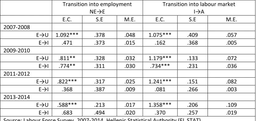
Table 3 presents the econometric results regarding the AWE for different time periods (2007-2008, 2009-2010, 2011-2012 and 2013-2014). This exercise will shed light on the evolution of the impact of husband’s labour market transitions on wife’s transitions into employment (ΝΕ→Ε) and the labour market (I→A). The specification of the econometric model include the variables that have been utilized in the estimation of the models presented on Table 2. We observe that the impact of husband’s job loss (E→U) in the period 2007-2008 is 4.8, in the period 2009-2011 is 3.2, in the period 2012-2013 is 2.5and in the period 2013-2014 is 1.7. Thus, in the course of time the AWE in the case of employment entry becomes weaker. This implies that as the macroeconomic environment worsens, the transition into employment becomes harder for those women with husbands that lost their jobs. However, in the case of labour market entry (I→A) these results follow opposing paths. In particular, we observe that the estimated impact of husband’s transition from employment to unemployment (E → U) for the period 2007-2008 is 5.7, for the period 2009-2011 is 7.2, for the period 2012-2013 is 8.2and for the period 2013-2014 is 10.9. Thus, over time, the impact of the AWE in the case of labour market entry becomes higher. This finding implies that as the economy slows down, the need for a stronger labour market attachment for those women with husbands who lost their jobs is more pronounced. Nevertheless, this need cannot be transformed into employment because of the prolonged economic crisis and the subsequent low job-finding rate (Daouli, et al. 2015). Thus, the pool of unemployed gets larger.

Insert Table 3 about here

(15)

13

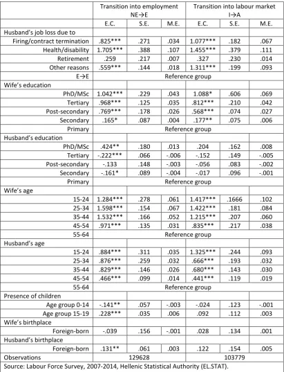
whenever the husband’s transition from the employment state to the non-employment one is considered to be low, then the AWE is practically non-existent. More specifically, the wife’s labour supply responsiveness regarding the transition NE→E is low when the husband is retired. Analogously, when the husband is getting out of employment for family-related reasons, the estimated AWE is small and stands at 1.8 percentage points. In contrast, when the husband lost his job due to firing or contract termination we observe that the wife’s transition probability of moving from the non-employment state to the unemployment one becomes larger. In particular, the estimated marginal effect indicates that women with laid-off husbands between the time period t-1 and t have 3.4 percentage points higher probability to become employed during the same time period. Of course, when the husband is leaving voluntarily the employment state due to health reasons, the wife’s probability of becoming employed increases by 10.7 percentage points. It should be noted that this marginal effect is much higher than the case where the husband has lost his job involuntarily (laid-off/contract termination). Assuming that the income loss due to health reasons is higher than the corresponding loess due to work-related involuntary separation reasons, the above findings imply that the wife’s labour supply responsiveness is increasing with the magnitude of the scheduled income loss at the household level. With regard to the effects of the remaining variables we do not observe any substantial differences than those presented in Table 2. From this point of view the estimated AWE is considered to be quite robust.

Regarding the transition from the inactivity state to the in-labour-force one (I→A) we observe that the estimated results are identical in terms of the direction of the effects with those results pertaining to the transition NE→E. However, they differ with regard to the magnitude of the estimated effect. More specifically, we observe that when the husband has lost his job during the period 𝑡 − 1 and 𝑡, the wife’s probability to enter the labour market is 11.1 percentage points higher than the case where the husband continues to be employed during that period. The same holds when the husband is resign due to family reasons (9.3 percentage points) and when the husband has lost his job due to firing or contract termination reasons.

(16)

14

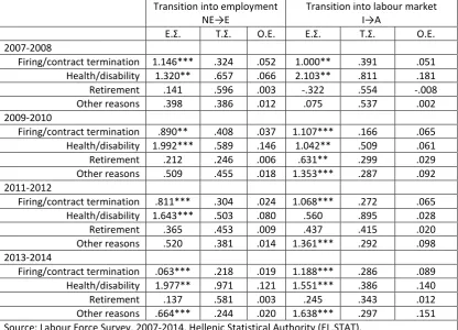
Table 5 presents the estimation results by slicing the dataset into sub-sample of a two-year period in order to find out how the AWE evolves over the crisis in Greece. Focusing only on the impact of the AWE we observe that the effect of husband’s transition from the employment state to the non-employment one on wife’s transition NE→E becomes lower over time. For instance, the estimated marginal effect is 5.2 for the period 2007-2008, 3.7 for the period 2009-2010, 2.4 for the period 2011-2012 and 1.9 for the period 2013-2014. At the same time the effects of husband’s job loss due to health/disability reasons follow a path with enormous variations (6.6 for the period 2007-2008, 14.6 for the period 2009-2010, 8.0 for the period 2011-2012 and for 12.1 for the period 2013-2014). Thus, the wife’s labour supply responsiveness to the income loss arsing from husband’s job loss due to health/disability reasons seems to be substantial but it does not follow a specific time path. However, the wife’s labour supply responsiveness to the income loss arsing from husband’s job loss due to firing/contract termination reasons seems to be significant but it follows a rather negative trend over time. Thus, as the economic crisis intensifies the AWE becomes weaker.

--Insert Table 5 about here --

(17)

15

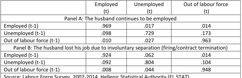
According to the estimated results, employed women in 𝑡 − 1 have a higher probability of being employed in 𝑡 when their husbands continue to be employed during this period. In addition, the transition probability from employment to unemployment is higher when the husband is involuntarily separated from their job (fired/contract termination) and thus the probability of exiting the labour market becomes smaller. In other words, an unemployed woman with an employed husband exerts a lower probability of exiting the labour market compared to a woman with a husband who lost his job due to involuntary separation. In this case, the unemployed woman faces an increasing risk of remaining unemployed for a prolonged period due to the low job-finding rate that characterize the Greek labour market in the post-2010 period. It is worth mentioning that the flows from the unemployment state to the employment one are of the same magnitude for both groups of women. With regard to the transition from the inactivity state in 𝑡 − 1 to the employment, unemployment or inactivity in 𝑡 we found that that women with involuntarily separated husbands have the same transition probability as those women with continuously employed husbands.

--Insert table 6 about here --

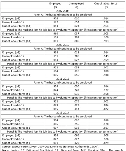
Table 7 presents the estimation results of the wife’s conditional transition probability matrices between 𝑡 − 1 and 𝑡 for a two-year period. Again these probabilities have been estimated for the tow alternative scenarios presented in Table 6. This exercise attempts to analyze the evolution of the “net” AWE over the course of the Greek economic crisis. We observe that women with husbands who involuntarily separated from their jobs face a lower probability of remaining in the employment state but an increasing probability of becoming unemployed (compared

to women with continuously employed husbands). With regard to the wife’s transition

(18)

16

probability of finding a job decreases substantially. This will have significant implications in the determination of the shadow wage and thus on the willingness to accept job offers with lower wage rates. This conclusion is reinforced by the results referring to the transition from the inactivity state to the activity one. In particular, we observe that the wife’s labour force participation is related to the unemployment state and not to the employment one. Women out of labour force with husbands who lost their jobs seem to face increased probabilities over time regarding the transition into unemployment (compared to those women with continuously employed husbands). This results in the decreasing persistence in the inactivity state.

-- Insert table 7 about here --

5. Conclusions

The present study investigates the wife’s labour supply responsiveness to the

husband’s job loss during the period 2007-2014 in Greece. For analytical purposes micro-data from the Labour Force Survey have been utilized. In order to examine the interrelated labour supply decisions of couples we exploited information on both spouses regarding labour market outcomes in the current period and in the period of 12 months before the survey. In this context, we were able to directly estimate that short-term response of wife’s labour supply to household’s income loss arising from the husband’s job loss. It has been documented extensively that involuntary job loss has a substantial negative effect on the individual labor market outcomes. This is of special importance since the labour market outcomes in Greece are severely deteriorated due to the economic downturn that has been demonstrated after the 2008 global economic crisis and the subsequent sovereign debt crisis. These developments exerted a negative impact on the employment dynamics of the Greek economy and thus at the aggregate level then unemployment rate increase considerably. At the same time the probability of moving from the employment state to the unemployment one has been also increased and in the case of married men it has doubled between 2007 and 2014 (0.7% and 2.8%, respectively).

(19)

17

participation becomes larger as the economic crisis deepens. However, this is not true for the case of employment entry where the AWE becomes practically insignificant. The above results are confirmed when the conditional transition probability matrices are estimated for every labour market transition and for women with and without husbands who lost their jobs. We also found that the increased rate of wife’s labour

force participation due to husband’s job loss is not directly converted into increased

employment rates. Instead, it converted directly into higher unemployment rates, a finding that intensifies as the employment conditions deteriorate. The above findings constitute strong indication for downward pressures in the determination of the shadow wage rate for married women in Greece.

The economic policy implications of these findings are worth mentioning. There is an increasing scope for public policy to facilitate employment creation in

order to minimize the period of household’s income loss due to husband’s job loss and

(20)

18

Bibliography

Ayhan H. S. (2015). Evidence of added worker effect from the 2008 economic crisis, IZA Discussion Paper No. 8937.

Baker, M. and Dwayne, B. (1997). The Role of the family in immigrants' labour- market activity: an evaluation of alternative explanations," American Economic Review, vol. 87(4), 705-27.

Bhalotra, S. and Umana-Aponte, M. (2010). The dynamics of women's labour supply in developing countries. IZA Discussion Paper, No. 4879.

Blundell, R. and Macurdy, T. (1999). Labour supply: A review of

alternative approaches," Handbook of Labour Economics, in: O. Ashenfelter& D. Card (ed.), Handbook of Labour Economics, edition 1, vol. 3, ch. 27, 1559-1695 Elsevier.

Bredtmann, J. Otten, S. and Rulff, C. (2014), Husband’s unemployment and wife’s labor supply-the added worker effect across Europe. Ruhr Economic Papers #484.

Chetty, R. and Szeidl, A. (2007). Consumption commitments and risk Preferences. Quarterly Journal of Economics, vol. 122(2), 831-877. Cobb-Clark, D. and Crossley, F.T. (2004). Revisiting the family

investment hypothesis. Labour Economics, vol. 11(3), 373-393.

Congregado, E. Golpe, A. and van Stel, A. (2011). Exploring the big jump in the Spanish unemployment rate: Evidence on an “added-worker” effect.

Economic Modelling, vol. 28(3), 1099-1105.

Cullen, J. and Gruber, J. (2000). Does unemployment insurance crowd

out spousal labour supply? Journal of Labour Economics, vol. 18(3), 546-572. Daouli, J. Demoussis, M. Giannakopoulos N. and Lampropoulou, N (2015) The ins

and outs of Greek unemployment in the Great Depression. University of Patras, mimeo.

Daouli, J. Demoussis, M. Giannakopoulos N. (2006). Child Care Costs and Employment Decisions of Greek Women, SSRN Working Paper Series. Available at SSRN: http://ssrn.com/abstract=917681.

Daouli, J. Demoussis, M. Giannakopoulos N. (2004). Participation of Greek

married women in full-time paid employment. South Eastern Europe Journal of Economics, vol. 2(2), 19-33.

Darby, J. Hart, R.A. and Vecchi, M. (2001) Labour force participation and the business cycle: a comparative analysis of France, Japan, Sweden and the United States.

Japan and the World Economy, vol. 13, 113–133.

Demoussis, M. and Giannakopoulos, N. (2008). Employment dynamics of Greek married women. International Journal of Manpower, 29(5), 423-442. Heckman, J.J. and MaCurdy, T. (1982). Corrigendum on a life cycle

model of female labour supply. Review of Economic Studies, vol. 49(4), 659-860.

Karaoglan, D. and Okten, C. (2015). Labor force participation of married

women in Turkey: a study of the added-worker effect and the discouraged-worker effect,Emerging Markets Finance and Trade, vol. 51(1), 274-290. Kuhn, P. and Schuetze, H. (2001). Self-employment dynamics and self-

employment trends: a study of Canadian men and women, 1982-1998,

(21)

19

Lundberg, S. (1985). The added worker effect," Journal of Labour Economics, vol. 3(1), 11-37.

Meghir, C. Ioannides, I. and Pissarides, C. (1989). Female participation and male

unemployment duration in Greece: evidence from the Labour Force Survey”,

European Economic Review, vol. 33, 395-406.

Mincer, J. (1962). Labour force participation of married women: a study of labour supply”, in Lewis, H.G. (ed.), Aspects of Labour Economics. NBER, Princeton University Press, 63-97.

Morissette, R. and Ostrovsky, Y. (2009). How do families and unattached individuals respond to layoffs? evidence from Canada," CLSRN Working Papers clsrn_admin-2009-49, UBC Department of Economics, revised 25 Sep 2009.

Moulton, B.R. (1986). Random group effects and the precision of regression Estimates. Journal of Econometrics, vol. 32, 385-97.

Nicolitsas, D. (2006). Female labour force participation in Greece. Bank of Greece Economic Bulletin, vol. 12, Bank of Greece, Athens.

OECD (2014). OECD Employment Outlook 2014, OECD Publishing. http://dx.doi.org/10.1787/empl_outlook-2014-en.

Parker, S. and Skoufias, E. (2004). The added worker effect over the business cycle: evidence from Mexico. Applied Economics Letters. vol. 11, 625–630.

Prieto-Rodríguez, J. and Rodríguez-Gutiérrez, C. (2003). Participation of married women in the European labor markets and the ‘‘added worker effect’’.

Journal of Socio-Economics, vol. 32 (4), 429–446.

Starr, M. A. (2014). Gender, added-worker effects, and the 2007-2009 recession: looking within the household. Review of Economics of the Household 12(2), 209–235.

Stephens, M. (2002). Worker displacement and the added worker effect. Journal of Labour Economics, vol. 20(3), 504-537.

Triebe, D. (2015). The added worker effect differentiated by gender and partnership status: Evidence from involuntary job loss, SOEPpapers on Multidisciplinary Panel Data Research, No. 740.

(22)

20

Figures

Figure 1. Unconditional probability of annual transition from employment to unemployment of married males in Greece (2007-2014)

Source: Labour Force Survey (LFS), Hellenic Statistical Authority (EL.STAT.).

[image:22.595.112.490.219.473.2]

(23)

21

[image:23.595.92.512.116.712.2]

Tables

Table 1. Means of wife’s characteristics by husband’s employment status

Husband’s employment status

Wife’s characteristics Employment Unemployment Out of labour force Employment status

Employment 56.66 42.48 25.12 Unemployment 9.05 29.15 3.82 Out of labour force 34.24 28.38 71.05 Education

PhD-MSc 1.68 1.00 0.32 Tertiary 22.84 14.70 10.65 Post-secondary 10.47 9.10 5.05

Secondary 45.76 51.49 36.60 Primary 19.24 23.71 47.38 Age groups

15-24 1.34 2.09 0.06 25-34 20.59 21.98 0.74 35-44 38.51 35.85 4.51 45-54 29.77 31.10 26.52 55-64 9.79 8.99 68.17 Family structure

Family size 3.43 3.50 2.77 Children in the age [0-14] 51.05 49.15 5.26 Children in the age [5-19] 20.37 20.72 6.27 Birthplace

Greece 88.61 73.49 96.43 Foreign-born 11.39 26.51 3.57 Region of Residence

Eastern Macedonia and Thrace 5.58 6.75 5.31 Central Macedonia (greater area) 9.17 8.67 9.52 Western Macedonia 2.38 2.75 2.99 Epirus 3.07 2.51 3.54 Thessaly 6.72 4.88 6.76 Ionian Islands 2.14 1.44 1.91 Western Greece 6.19 5.51 6.25 East and Central Greece 5.00 4.09 5.62 Attica (greater area) 4.85 5.30 5.06 Peloponnese 5.36 3.16 5.11 Northern Aegean 1.78 1.15 1.99 Southern Aegean 2.95 2.97 2.73 Grete 5.79 5.01 4.92 Attica (Athens) 30.68 35.09 30.27 Central Macedonia (Salonica) 8.35 10.72 8.02 Degree of urbanization (residence area)

Urban 66.41 73.76 64.48 Semi-urban 13.79 12.48 14.11 Rural 19.80 13.76 21.41 Source: Labour Force Survey, 2007-2014, Hellenic Statistical Authority (EL.STAT).

(24)

22

Table 2. The impact of the AWE on wife’s transitions into employment and the labour market

Transition into employment

NE→E

Transition into labour market

I→A

E.C. S.E M.E. E.C. S.E M.E.

Husband’s transitions

E→U .784*** .267 .028 1.211*** .132 .080

E→I .613*** .178 .020 .364** .171 .016

E→E Reference group

Wife’s education

PhD/MSc 1.031*** .232 .043 1.087* .604 .069 Tertiary .966*** .125 .035 .811*** .210 .042 Post-secondary .764*** .178 .026 .568*** .074 .027 Secondary .162* .087 .004 .174** .075 .006

Primary Reference group

Husband’s education

PhD/MSc .420** .183 .013 .200 .162 .008 Tertiary -.227*** .066 -.006 -.154 .149 -.005 Post-secondary -.139 .148 -.003 -.052 .083 -.002 Secondary -.164* .089 -.004 -.017 .096 -.001

Wife’s age

15-24 1.302*** .282 .061 1.411*** .1666 .102 25-34 1.617*** .149 .067 1.421*** .181 .084 35-44 1.532*** .164 .052 1.217*** .207 .060 45-54 .990*** .136 .031 .840*** .228 .038 55-64 Reference group

Husband’s age

15-24 .910*** .311 .035 1.308*** .244 .093 25-34 .902*** .255 .032 .658*** .206 .032 35-44 .855*** .143 .026 .674*** .156 .030 45-54 .493*** .097 .014 .438*** .128 .019 55-64 Reference group

Presence of children

Age group 0-14 -.139** .057 -.003 -.023 .122 -.001 Age group 15-19 .230*** .035 .006 .090 .114 .003

Wife’s birthplace

Foreign-born -.037 .158 -.001 .027 .132 .001

husband’s birthplace

Foreign-born .133** .059 .003 .116 .157 .005

Observations 129628 103779

Source: Labour Force Survey, 2007-2014, Hellenic Statistical Authority (EL.STAT).

(25)

[image:25.595.90.511.134.332.2]

23

Table 3. The impact of the AWE on wife’s transitions into employment and the labour market for different time periods

NE→E

Transition into labour market I→A

E.C. S.E M.E. E.C. S.E M.E. 2007-2008

E→U 1.092*** .378 .048 1.075*** .409 .057

E→I .471 .373 .015 .162 .368 .005 2009-2010

E→U .811** .328 .032 1.179*** .133 .072 E→I .774** .311 .030 .734*** .231 .036 2011-2012

E→U .822*** .317 .025 1.241*** .151 .082

E→I .368 .387 .009 .081 .266 .003 2013-2014

E→U .588*** .213 .017 1.358*** .206 .109

E→I .683 .494 .020 .370 .257 .019 Source: Labour Force Survey, 2007-2014, Hellenic Statistical Authority (EL.STAT).

(26)

[image:26.595.90.502.109.647.2]

24

Table 4. The impact of the AWE on wife’s transitions into employment and the labour

market by reason of husband’s job loss

NE→E

Transition into labour market I→A

E.C. S.E. M.E. E.C. S.E. M.E.

Husband’s job loss due to

Firing/contract termination .825*** .271 .034 1.077*** .182 .067 Health/disability 1.705*** .388 .107 1.455*** .379 .111 Retirement .259 .217 .007 .327 .230 .014 Other reasons .559*** .144 .018 1.311*** .199 .093

E→E Reference group

Wife’s education

PhD/MSc 1.042*** .229 .043 1.088* .606 .069 Tertiary .968*** .125 .035 .812*** .210 .042 Post-secondary .769*** .178 .026 .568*** .074 .027 Secondary .165* .087 .004 .177** .075 .006

Husband’s education

PhD/MSc .424** .180 .013 .204 .162 .008 Tertiary -.222*** .066 -.006 -.152 .149 -.005 Post-secondary -.133 .148 -.003 -.056 .083 -.002 Secondary -.161* .089 -.004 -.017 .096 -.001

Wife’s age

15-24 1.284*** .278 .061 1.417*** .1666 .102 25-34 1.598*** .154 .067 1.422*** .181 .084 35-44 1.532*** .166 .052 1.215*** .207 .060 45-54 .971*** .135 .031 .835*** .217 .038 55-64 Reference group

Husband’s age

15-24 .884*** .311 .035 1.325*** .244 .093 25-34 .876*** .259 .032 .666*** .193 .032 35-44 .829*** .146 .026 .680*** .143 .030 45-54 .466*** .099 .014 .441*** .119 .019 55-64 Reference group

Presence of children

Age group 0-14 -.141** .057 -.003 -.024 .123 -.001 Age group 15-19 .228*** .035 .006 .092 .112 .003

Wife’s birthplace

Foreign-born -.039 .156 -.001 .028 .134 .001

Husband’s birthplace

Foreign-born .131** .061 .003 .122 .154 .005

Observations 129628 103779

Source: Labour Force Survey, 2007-2014, Hellenic Statistical Authority (EL.STAT).

(27)

[image:27.595.92.509.135.435.2]

25

Table 5. The impact of the AWE on wife’s transitions into employment and the labour market by reason of husband’s job loss and time period

Transition into employment NE→E

Transition into labour market

I→A

Ε.Σ. Τ.Σ. Ο.Ε. Ε.Σ. Τ.Σ. Ο.Ε.

2007-2008

Firing/contract termination 1.146*** .324 .052 1.000** .391 .051 Health/disability 1.320** .657 .066 2.103** .811 .181 Retirement .141 .596 .003 -.322 .554 -.008 Other reasons .398 .386 .012 .075 .537 .002 2009-2010

Firing/contract termination .890** .408 .037 1.107*** .166 .065 Health/disability 1.992*** .589 .146 1.042** .509 .061 Retirement .212 .246 .006 .631** .299 .029 Other reasons .509 .455 .018 1.353*** .287 .092 2011-2012

Firing/contract termination .811*** .304 .024 1.068*** .272 .065 Health/disability 1.643*** .503 .080 .560 .895 .028 Retirement .365 .453 .009 .437 .415 .020 Other reasons .520 .381 .014 1.361*** .292 .098 2013-2014

Firing/contract termination .063*** .218 .019 1.188*** .286 .089 Health/disability 1.977** .971 .121 1.551*** .386 .140 Retirement .137 .581 .003 .245 .343 .012 Other reasons .664*** .244 .020 1.638*** .297 .151 Source: Labour Force Survey, 2007-2014, Hellenic Statistical Authority (EL.STAT).

(28)

[image:28.595.89.511.148.284.2]

26

Table 6. Estimated transition probabilities by economic activity statuses for women with employed husbands and husbands who lost their jobs due to involuntary separation

Employed (t)

Unemployed (t)

Out of labour force (t) Panel A: The husband continues to be employed

Employed (t-1) .969 .017 .014 Unemployed (t-1) .098 .729 .173 Out of labour force (t-1) .010 .027 .963

Panel B: The husband lost his job due to involuntary separation (firing/contract termination) Employed (t-1) .924 .062 .014 Unemployed (t-1) .092 .804 .104 Out of labour force (t-1) .008 .044 .948 Source: Labour Force Survey, 2007-2014, Hellenic Statistical Authority (EL.STAT).

(29)

[image:29.595.88.512.121.630.2]

27

Table 7. Estimated transition probabilities by economic activity statuses for women with employed husbands and husbands who lost their jobs due to involuntary separation for different time periods

Employed (t)

Unemployed (t)

Out of labour force (t) 2007-2008

Panel A: The husband continues to be employed

Panel B: The husband lost his job due to involuntary separation (firing/contract termination) Employed (t-1) .960 .037 .003 Unemployed (t-1) .103 .797 .100 Out of labour force (t-1) .001 .006 .993

2009-2010

2011-2012

2013-2014

Panel B: The husband lost his job due to involuntary separation (firing/contract termination) Employed (t-1) .926 .066 .008 Unemployed (t-1) .072 .822 .106 Out of labour force (t-1) .001 .120 .879 Source: Labour Force Survey, 2007-2014, Hellenic Statistical Authority (EL.STAT).