Improved Discriminative Bilingual Word Alignment
Robert C. Moore Wen-tau Yih Andreas Bode Microsoft Research
Redmond, WA 98052, USA
{bobmoore,scottyhi,abode}@microsoft.com
Abstract
For many years, statistical machine trans-lation relied on generative models to pro-vide bilingual word alignments. In 2005, several independent efforts showed that discriminative models could be used to enhance or replace the standard genera-tive approach. Building on this work, we demonstrate substantial improvement in word-alignment accuracy, partly though improved training methods, but predomi-nantly through selection of more and bet-ter features. Our best model produces the lowest alignment error rate yet reported on Canadian Hansards bilingual data.
1 Introduction
Until recently, almost all work in statistical ma-chine translation was based on word alignments obtained from combinations of generative prob-abalistic models developed at IBM by Brown et al. (1993), sometimes augmented by an HMM-based model or Och and Ney’s “Model 6” (Och and Ney, 2003). In 2005, however, several in-dependent efforts (Liu et al., 2005; Fraser and Marcu, 2005; Ayan et al., 2005; Taskar et al., 2005; Moore, 2005; Ittycheriah and Roukos, 2005) demonstrated that discriminatively trained models can equal or surpass the alignment accu-racy of the standard models, if the usual unla-beled bilingual training corpus is supplemented with human-annotated word alignments for only a small subset of the training data.
The work cited above makes use of various training procedures and a wide variety of features. Indeed, whereas it can be difficult to design a fac-torization of a generative model that incorporates
all the desired information, it is relatively easy to add arbitrary features to a discriminative model. We take advantage of this, building on our ex-isting framework (Moore, 2005), to substantially reduce the alignment error rate (AER) we previ-ously reported, given the same training and test data. Through a careful choice of features, and modest improvements in training procedures, we obtain the lowest error rate yet reported for word alignment of Canadian Hansards data.
2 Overall Approach
As in our previous work (Moore, 2005), we train two models we call stage 1 and stage 2, both in the form of a weighted linear combination of fea-ture values extracted from a pair of sentences and a proposed word alignment of them. The possible alignment having the highest overall score is se-lected for each sentence pair. Thus, for a sentence pair(e, f)we seek the alignmentˆasuch that
ˆ
a= argmaxa
n
X
i=1
λifi(a, e, f)
where the fi are features and theλi are weights.
The models are trained on a large number of bilin-gual sentence pairs, a small number of which have hand-created word alignments provided to the training procedure. A set of hand alignments of a different subset of the overall training corpus is used to evaluate the models.
In the stage 1 model, all the features are based on surface statistics of the training data, plus the hypothesized alignment. The entire training cor-pus is then automatically aligned using this model. The stage 2 model uses features based not only on the parallel sentences themselves but also on statistics of the alignments produced by the stage
1 model. The stage 1 model is discussed in Sec-tion 3, and the stage 2 model, in SecSec-tion 4. After experimenting with many features and combina-tions of features, we made the final selection based on minimizing training set AER.
For alignment search, we use a method nearly identical to our previous beam search procedure, which we do not discuss in detail. We made two minor modifications to handle the possiblity that more than one alignment may have the same score, which we previously did not take into account. First, we modified the beam search so that the beam size dynamically expands if needed to ac-comodate all the possible alignments that have the same score. Second we implemented a structural tie breaker, so that the same alignment will always be chosen as the one-best from a set of alignments having the same score. Neither of these changes significantly affected the alignment results.
The principal training method is an adaptation of averaged perceptron learning as described by Collins (2002). The differences between our cur-rent and earlier training methods mainly address the observation that perceptron training is very sensitive to the order in which data is presented to the learner. We also investigated the large-margin training technique described by Tsochantaridis et al. (2004). The training procedures are described in Sections 5 and 6.
3 Stage 1 Model
In our previous stage 1 model, we used five fea-tures. The most informative feature was the sum of bilingual word-association scores for all linked word pairs, computed as a log likelihood ratio. We used two features to measure the degree of non-monotonicity of alignments, based on traversing the alignment in the order of the source sentence tokens, and noting the instances where the corre-sponding target sentence tokens were not in left-to-right order. One feature counted the number of times there was a backwards jump in the order of the target sentence tokens, and the other summed the magnitudes of these jumps. In order to model the trade-off between one-to-one and many-to-one alignments, we included a feature that counted the number of alignment links such that one of the linked words participated in another link. Our fifth feature was the count of the number of words in the sentence pair left unaligned.
In addition to these five features, we employed
two hard constraints. One constraint was that the only alignment patterns allowed were 1–1, 1–2, 1– 3, 2–1, and 3–1. Thus, many-to-many link pat-terns were disallowed, and a single word could be linked to at most three other words. The second constraint was that a possible link was considered only if it involved the strongest degree of associ-ation within the sentence pair for at least one of the words to be linked. If both words had stronger associations with other words in the sentence pair, then the link was disallowed.
Our new stage 1 model includes all the features we used previously, plus the constraint on align-ment patterns. The constraint involving strongest association is not used. In addition, our new stage 1 model employs the following features:
association score rank features We define the rank of an association with respect to a word in a sentence pair to be the number of association types (word-type to word-type) for that word that have higher association scores, such that words of both types occur in the sentence pair. The contraint on strength of association we previously used can be stated as a requirement that no link be considered unless the corresponding association is of rank 0 for at least one of the words. We replace this hard constraint with two features based on association rank. One feature totals the sum of the associa-tion ranks with respect to both words involved in each link. The second feature sums the minimum of association ranks with respect to both words in-volved in each link. For alignments that obey the previous hard constraint, the value of this second feature would always be 0.
source words and the distance between the closest target words they are aligned to.
many-to-one jump distance features It seems intuitive that the likelihood of a large forward jump on either the source or target side of an align-ment is much less if the jump is between words that are both linked to the same word of the other language. This motivates the distinction between thed1andd>1parameters in IBM Models 4 and 5.
We model this by including two features. One fea-ture sums, for each wordw, the number of words not linked towthat fall between the first and last words linked tow. The other features counts only such words that are linked to some word other than
w. The intuition here is that it is not so bad to have a function word not linked to anything, between two words linked to the same word.
exact match feature We have a feature that sums the number of words linked to identical words. This is motivated by the fact that proper names or specialized terms are often the same in both languages, and we want to take advantage of this to link such words even when they are too rare to have a high association score.
lexical features Taskar et al. (2005) gain con-siderable benefit by including features counting the links between particular high frequency words. They use 25 such features, covering all pairs of the five most frequent non-punctuation words in each language. We adopt this type of feature but do so more agressively. We include features for all bilingual word pairs that have at least two co-occurrences in the labeled training data. In addi-tion, we include features counting the number of unlinked occurrences of each word having at least two occurrences in the labeled training data.
In training our new stage 1 model, we were con-cerned that using so many lexical features might result in overfitting to the training data. To try to prevent this, we train the stage 1 model by first timizing the weights for all other features, then op-timizing the weights for the lexical features, with the other weights held fixed to their optimium val-ues without lexical features.
4 Stage 2 Model
In our original stage 2 model, we replaced the log-likelihood-based word association statistic with the logarithm of the estimated conditional prob-ability of a cluster of words being linked by the
stage 1 model, given that they co-occur in a pair of aligned sentences, computed over the full (500,000 sentence pairs) training data. We esti-mated these probabilities using a discounted max-imum likelihood estimate, in which a small fixed amount was subtracted from each link count:
LPd(w1, . . . , wk) =
links1(w1, . . . , wk)−d cooc(w1, . . . , wk)
LPd(w1, . . . , wk) represents the estimated
condi-tional link probability for the cluster of words
w1, . . . , wk;links1(w1, . . . , wk)is the number of times they are linked by the stage 1 model, d is the discount; andcooc(w1, . . . , wk)is the number
of times they co-occur. We found that d = 0.4
seemed to minimize training set AER.
An important difference between our stage 1 and stage 2 models is that the stage 1 model con-siders each word-to-word link separately, but al-lows multiple links per word, as long as they lead to an alignment consisting only of one-to-one and one-to-many links (in either direction). The stage 2 model, however, uses conditional probabilities for both one-to-one and one-to-many clusters, but requires all clusters to be disjoint. Our original stage 2 model incorporated the same addtional fea-tures as our original stage 1 model, except that the feature that counts the number of links involved in non-one-to-one link clusters was omitted.
Our new stage 2 model differs in a number of ways from the original version. First we replace the estimated conditional probability of a cluster of words being linked with the estimated condi-tional odds of a cluster of words being linked:
LO(w1, . . . , wk) =
links1(w1, . . . , wk) + 1
(cooc(w1, . . . , wk)−links1(w1, . . . , wk)) + 1
LO(w1, . . . , wk) represents the estimated
con-ditional link odds for the cluster of words
w1, . . . , wk. Note that we use “add-one”
smooth-ing in place of a discount.
Additional features in our new stage 2 model in-clude the unaligned word feature used previously, plus the following features:
sentence order, with the sum of the backwards jumps in the source sentence order relative to the target sentence order. We omit the feature that counts the number of backwards jumps.
multi-link feature This feature counts the num-ber of link clusters that are not one-to-one. This enables us to model whether the link scores for these clusters are more or less reliable than the link scores for one-to-one clusters.
empirically parameterized jump distance fea-ture We take advantage of the stage 1 alignment to incorporate a feature measuring the jump dis-tances between alignment links that are more so-phisticated than simply measuring the difference in source and target distances, as in our stage 1 model. We measure the (signed) source and target distances between all pairs of links in the stage 1 alignment of the full training data. From this, we estimate the odds of each possible target distance given the corresponding source distance:
J O(dt|ds) =
C(target dist=dt∧source dist=ds) + 1 C(target dist6=dt∧source dist=ds) + 1
We similarly estimate the odds of each possi-ble source distance given the corresponding target distance. The feature values consist of the sum of the scaled log odds of the jumps between con-secutive links in a hypothesized alignment, com-puted in both source sentence and target sentence order. This feature is applied only when both the source and target jump distances are non-zero, so that it applies only to jumps between clusters, not to jumps on the “many” side of a many-to-one cluster. We found it necessary to linearly scale these feature values in order to get good results (in terms of training set AER) when using perceptron training.1 We found empirically that we could get good results in terms of training set AER by divid-ing each log odds estimate by the largest absolute value of any such estimate computed.
5 Perceptron Training
We optimize feature weights using a modification of averaged perceptron learning as described by Collins (2002). Given an initial set of feature weight values, the algorithm iterates through the
1Note that this is purely for effective training, since after training, one could adjust the feature weights according to the scale factor, and use the original feature values.
labeled training data multiple times, comparing, for each sentence pair, the best alignmentahyp
ac-cording to the current model with the reference alignmentaref. At each sentence pair, the weight
for each feature is is incremented by a multiple of the difference between the value of the feature for the best alignment according to the model and the value of the feature for the reference alignment:
λi ←λi+η(fi(aref, e, f)−fi(ahyp, e, f))
The updated feature weights are used to compute
ahyp for the next sentence pair. The multiplier η
is called the learning rate. In the averaged percep-tron, the feature weights for the final model are the average of the weight values over all the data rather than simply the values after the final sen-tence pair of the final iteration.
Differences between our approach and Collins’s include averaging feature weights over each pass through the data, rather than over all passes; ran-domizing the order of the data for each learn-ing pass; and performlearn-ing an evaluation pass af-ter each learning pass, with feature weights fixed to their average values for the preceding learning pass, during which training set AER is measured. This procedure is iterated until a local minimum on training set AER is found.
We initialize the weight of the anticipated most-informative feature (word-association scores in stage 1; conditional link probabilities or odds in stage 2) to 1.0, with other feature weights intial-ized to 0. The weight for the most informative fea-ture is not updated. Allowing all weights to vary allows many equivalent sets of weights that differ only by a constant scale factor. Fixing one weight eliminates a spurious apparent degree of freedom. Previously, we set the learning rateηdifferently in training his stage 1 and stage 2 models. For the stage 2 model, we used a single learning rate of 0.01. For the stage 1 model, we used a sequence of learning rates: 1000, 100, 10, and 1.0. At each transition between learning rates, we re-initialized the feature weights to the optimum values found with the previous learning rate.
stage 2 models, setting the learning rates automat-ically. The initial learning rate is the maximum ab-solute value (for one word pair/cluster) of the word association, link probability, or link odds feature, divided by the number of labeled training sentence pairs. Since many of the feature values are simple counts, this allows a minimal difference of 1 in the feature value, if repeated in every training ex-ample, to permit a count feature to have as large a weighted value as the most informative feature, after a single pass through the data.
After the learning search terminates for a given learning rate, we reduce the learning rate by a fac-tor of 10, and iterate until we judge that we are at a local minimum for this learning rate. We con-tinue with progressively smaller learning rates un-til an entire pass through the data produces fea-ture weights that differ so little from their values at the beginning of the pass that the training set AER does not change.
Two final modifications are inspired by the real-ization that the results of perceptron training are very sensitive to the order in which the data is presented. Since we randomize the order of the data on every pass, if we make a pass through the training data, and the training set AER increases, it may be that we simply encountered an unfortunate ordering of the data. Therefore, when training set AER increases, we retry two additional times with the same initial weights, but different random or-derings of the data, before giving up and trying a smaller learning rate. Finally, we repeat the entire training process multiple times, and average the feature weights resulting from each of these runs. We currently use 10 runs of each model. This final averaging is inspired by the idea of “Bayes-point machines” (Herbrich and Graepel, 2001).
6 SVM Training
After extensive experiments with perceptron train-ing, we wanted to see if we could improve the re-sults obtained with our best stage 2 model by using a more sophisticated training method. Perceptron training has been shown to obtain good results for some problems, but occasionally very poor results are reported, notably by Taskar et al. (2005) for the word-alignment problem. We adopted the support vector machine (SVM) method for structured out-put spaces of Tsochantaridis et al. (2005), using Joachims’SV Mstructpackage.
Like standard SVM learning, this method tries
to find the hyperplane that separates the training examples with the largest margin. Despite a very large number of possible output labels (e.g., all possible alignments of a given pair of sentences), the optimal hyperplane can be efficiently approx-imated given the desired error rate, using a cut-ting plane algorithm. In each iteration of the al-gorithm, it adds the “best” incorrect predictions given the current model as constraints, and opti-mizes the weight vector subject only to them.
The main advantage of this algorithm is that it does not pose special restrictions on the out-put structure, as long as “decoding” can be done efficiently. This is crucial to us because sev-eral features we found very effective in this task are difficult to incorporate into structured learning methods that require decomposable features. This method also allows a variety of loss functions, but we use only simple 0-1 loss, which in our case means whether or not the alignment of a sentence pair is completely correct, since this worked as well as anything else we tried.
Our SVM method has a number of free param-eters, which we tried tuning in two different ways. One way is minimizing training set AER, which is how we chose the stopping points in perceptron training. The other is five-fold cross validation. In this method, we train five times on 80% of the training data and test on the other 20%, with five disjoint subsets used for testing. The parameter values yielding the best averaged AER on the five test subsets of the training set are used to train the final model on the entire training set.
7 Evaluation
We used the same training and test data as in our previous work, a subset of the Canadian Hansards bilingual corpus supplied for the bilingual word alignment workshop held at HLT-NAACL 2003 (Mihalcea and Pedersen, 2003). This subset com-prised 500,000 English-French sentences pairs, in-cluding 224 manually word-aligned sentence pairs for labeled training data, and 223 labeled sen-tences pairs as test data. Automatic sentence alignment of the training data was provided by Ul-rich Germann, and the hand alignments of the la-beled data were created by Franz Och and Her-mann Ney (Och and Ney, 2003).
Alignment Recall Precision AER
Prev LLR 0.829 0.848 0.160
CLP1 0.889 0.934 0.086
CLP2 0.898 0.947 0.075
Giza E→F 0.870 0.890 0.118
Giza F→E 0.876 0.907 0.106
Giza union 0.929 0.845 0.124
Giza intersection 0.817 0.981 0.097
[image:6.595.73.291.61.187.2]Giza refined 0.908 0.929 0.079
Table 1: Baseline Results.
package, using the default configuration file (Och and Ney, 2003).2 “Prev LLR” is our earlier stage 1 model, and CLP1 and CLP2 are two versions of our earlier stage 2 model. For CLP1, condi-tional link probabilities were estimated from the alignments produced by our “Prev LLR” model, and for CLP2, they were obtained from a yet earlier, heuristic alignment model. Results for IBM Model 4 are reported for models trained in both directions, English-to-French and French-to-English, and for the union, intersection, and what Och and Ney (2003) call the “refined” combina-tion of the those two alignments.
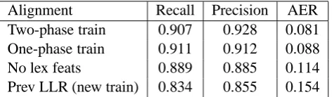
Results for our new stage 1 model are presented in Table 2. The first line is for the model described in Section 3, optimizing non-lexical features be-fore lexical features. The second line gives results for optimizing all features simultaneously. The next line omits lexical features entirely. The last line is for our original stage 1 model, but trained using our improved perceptron training method.
As we can see, our best stage 1 model reduces the error rate of previous stage 1 model by almost half. Comparing the first two lines shows that two-phase training of non-lexical and lexical features produces a 0.7% reduction in test set error. Al-though the purpose of the two-phase training was to mitigate overfitting to the training data, we also found training set AER was reduced (7.3% vs. 8.8%). Taken all together, the results show a 7.9% total reduction in error rate: 4.0% from new non-lexical features, 3.3% from non-lexical features with two-phase training, and 0.6% from other improve-ments in perceptron training.
Table 3 presents results for perceptron training of our new stage 2 model. The first line is for the model as described in Section 4. Since the use of log odds is somewhat unusual, in the second line
2
Thanks to Chris Quirk for providing Giza++ alignments.
Alignment Recall Precision AER
Two-phase train 0.907 0.928 0.081
One-phase train 0.911 0.912 0.088
No lex feats 0.889 0.885 0.114
Prev LLR (new train) 0.834 0.855 0.154
Table 2: Stage 1 Model Results.
Alignment Recall Precision AER
Log odds 0.935 0.964 0.049
Log probs 0.934 0.962 0.051
CLP1(new A & T) 0.925 0.952 0.060
[image:6.595.308.546.63.132.2]CLP1(new A) 0.917 0.955 0.063
Table 3: Stage 2 Model Results.
we show results for a similiar model, but using log probabilities instead of log odds for both the link model and the jump model. This result is 0.2% worse than the log-odds-based model, but the dif-ference is small enough to warrant testing its sig-nificance. Comparing the errors on each test sen-tence pair with a 2-tailed pairedttest, the results were suggestive, but not significant (p= 0.28)
The third line of Table 3 shows results for our earlier CLP1 model with probabilities estimated from our new stage 1 model alignments (“new A”), using our recent modifications to perceptron training (“new T”). These results are significantly worse than either of the two preceding models (p < 0.0008). The fourth line is for the same model and stage 1 alignments, but with our earlier perceptron training method. While the results are 0.3% worse than with our new training method, the difference is not significant (p= 0.62).
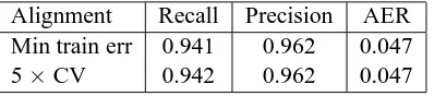
Table 4 shows the results of SVM training of the model that was best under perceptron training, tuning free parameters either by minimizing error on the entire training set or by 5-fold cross val-idation on the training set. The cross-valval-idation method produced slightly lower test-set AER, but both results rounded to 4.7%. While these results are somewhat better than with perceptron training, the differences are not significant (p≥0.47).
8 Comparisons to Other Work
Alignment Recall Precision AER
Min train err 0.941 0.962 0.047
[image:7.595.84.283.62.106.2]5×CV 0.942 0.962 0.047
Table 4: SVM Training Results.
total training data, labeled training data, and test data. The best previously reported result was by Och and Ney (2003), who obtained 5.2% AER for a combination including all the IBM mod-els except Model 2, plus the HMM model and their Model 6, together with a bilingual dictionary, for the refined alignment combination, trained on three times as much data as we used.
Cherry and Lin’s (2003) method obtained an AER of 5.7% as reported by Mihalcea and Peder-sen (2003), the previous lowest reported error rate for a method that makes no use of the IBM mod-els. Cherry and Lin’s method is similar to ours in using explicit estimates of the probability of a link given the co-occurence of the linked words; but it is generative rather than discriminative, it re-quires a parser for the English side of the corpus, and it does not model many-to-one links. Taskar et al. (2005) reported 5.4% AER for a discrimina-tive model that includes predictions from the inter-section of IBM Model 4 alignments as a feature. Their best result without using information from the IBM models was 10.7% AER.
After completing the experiments described in Section 7, we became aware further developments in the line of research reported by Taskar et al. (Lacoste-Julien et al., 2006). By modifying their previous approach to allow many-to-one ments and first-order interactions between align-ments, Lacoste-Julien et al. have improved their best AER without using information from the more complex IBM models to 6.2%. Their best result, however, is obtained from a model that in-cludes both a feature recording intersected IBM Model 4 predictions, plus a feature whose val-ues are the alignment probabilities obtained from a pair of HMM alignment models trained in both di-rections in such a way that they agree on the align-ment probabilities (Liang et al., 2006). With this model, they obtained a much lower 3.8% AER.
Lacoste-Julien very graciously provided both the IBM Model 4 predictions and the probabili-ties estimated by the bidirectional HMM models that they had used to compute these additional fea-ture values. We then added feafea-tures based on this
information to see how much we could improve our best model. We also eliminated one other dif-ference between our results and those of Lacoste-Julien et al., by training on all 1.1 million English-French sentence pairs from the 2003 word align-ment workshop, rather than the 500,000 sentence pairs we had been using.
Since all our other feature values derived from probabilities are expressed as log odds, we also converted the HMM probabilities estimated by Liang et al. to log odds. To make this well de-fined in all cases, we thresholded high probabili-ties (including 1.0) at 0.999999, and low probabil-ities (including 0.0) at 0.1 (which we found pro-duced lower training set error than using a very small non-zero probability, although we have not searched systematically for the optimal value).
In our latest experiments, we first established that simply increasing the unlabled training data to 1.1 million sentence pairs made very little dif-ference, reducing the test-set AER of our stage 2 model under perceptron training only from 4.9% to 4.8%. Combining our stage 2 model features with the HMM log odds feature using SVM train-ing with 5-fold cross validation yielded a substan-tial reduction in test-set AER to 3.9% (96.9% pre-cision, 95.1% recall). We found it somewhat dif-ficult to improve these results further by including IBM Model 4 intersection feature. We finally ob-tained our best results, however, for both training-set and test-training-set AER, by holding the stage 2 model feature weights at the values obtained by SVM training with the HMM log odds feature, and op-timizing the HMM log odds feature weight and IBM Model 4 intersection feature weight with per-ceptron training.3 This produced a test-set AER of 3.7% (96.9% precision, 95.5% recall).
9 Conclusions
For Canadian Hansards data, the test-set AER of 4.7% for our stage 2 model is one of the lowest yet reported for an aligner that makes no use of the expensive IBM models, and our test-set AER of 3.7% for the stage 2 model in combination with the HMM log odds and Model 4 intersection fea-tures is the lowest yet reported for any aligner.4
Perhaps if any general conclusion is to be drawn from our results, it is that in creating a
discrim-3
At this writing we have not yet had time to try this with SVM training.
inative word alignment model, the model struc-ture and feastruc-tures matter the most, with the dis-criminative training method of secondary impor-tance. While we obtained a small improvements by varying the training method, few of the differ-ences were statistically significant. Having better features was much more important.
References
Necip Fazil Ayan, Bonnie J. Dorr, and Christof Monz. 2005. NeurAlign: Combining Word Alignments Using Neural Networks. In Proceedings of the Human Language Technol-ogy Conference and Conference on Empirical Methods in Natural Language Processing, pp. 65–72, Vancouver, British Columbia.
Peter F. Brown, Stephen A. Della Pietra, Vincent J. Della Pietra, and Robert L. Mercer. 1993. The Mathematics of Statistical Machine Translation: Parameter Estimation. Computational Linguis-tics, 19(2):263–311.
Colin Cherry and Dekang Lin. 2003. A Proba-bility Model to Improve Word Alignment. In Proceedings of the 41st Annual Meeting of the ACL, pp. 88–95, Sapporo, Japan.
Michael Collins. 2002. Discriminative Training Methods for Hidden Markov Models: Theory and Experiments with Perceptron Algorithms. In Proceedings of the Conference on Empiri-cal Methods in Natural Language Processing, pp. 1–8, Philadelphia, Pennsylvania.
Alexander Fraser and Daniel Marcu. 2005. ISI’s Participation in the Romanian-English Align-ment Task. In Proceedings of the ACL Work-shop on Building and Using Parallel Texts, pp. 91–94, Ann Arbor, Michigan.
Ralf Herbrich and Thore Graepel. 2001. Large Scale Bayes Point Machines Advances. In Neural Information Processing Systems 13, pp. 528–534.
Abraham Ittycheriah and Salim Roukos. 2005. A Maximum Entropy Word Aligner for Arabic-English Machine Translation. In Proceedings of the Human Language Technology Conference and Conference on Empirical Methods in Nat-ural Language Processing, pp. 89–96, Vancou-ver, British Columbia.
Simon Lacoste-Julien, Ben Taskar, Dan Klein, and Michael Jordan. 2006. Word Alignment via Quadratic Assignment. In Proceedings of the Human Language Technology Conference of the North American Chapter of the Association for Computational Linguistics, pp. 112–119, New York City.
Percy Liang, Ben Taskar, and Dan Klein. 2006. Alignment by Agreement. In Proceedings of the Human Language Technology Conference of the North American Chapter of the Association for Computational Linguistics, pp. 104–111, New York City.
Yang Liu, Qun Liu, and Shouxun Lin. 2005. Log-linear Models for Word Alignment. In Proceed-ings of the 43rd Annual Meeting of the ACL, pp. 459–466, Ann Arbor, Michigan.
Rada Mihalcea and Ted Pedersen. 2003. An Eval-uation Exercise for Word Alignment. In Pro-ceedings of the HLT-NAACL 2003 Workshop, Building and Using Parallel Texts: Data Driven Machine Translation and Beyond, pp. 1–6, Ed-monton, Alberta.
Robert C. Moore. 2005. A Discriminative Frame-work for Bilingual Word Alignment. In Pro-ceedings of the Human Language Technology Conference and Conference on Empirical Meth-ods in Natural Language Processing, pp. 81– 88, Vancouver, British Columbia.
Franz Joseph Och and Hermann Ney. 2003. A Systematic Comparison of Various Statistical Alignment Models. Computational Linguistics, 29(1):19–51.
Ben Taskar, Simon Lacoste-Julien, and Dan Klein. 2005. A Discriminative Matching Approach to Word Alignment. In Proceedings of the Human Language Technology Conference and Conference on Empirical Methods in Natural Language Processing, pp. 73–80, Vancouver, British Columbia.
Ioannis Tsochantaridis, Thomas Hofmann, Thorsten Joachims, and Yasemin Altun. 2005. Large Margin Methods for Structured and Interdependent Output Variables. Journal
of Machine Learning Research (JMLR),