Munich Personal RePEc Archive
Disability Insurance Benefits and Labor
Supply Decisions: Evidence from a
Discontinuity in Benefit Awards
Müller, Tobias and Boes, Stefan
University of Lucerne, University of Lucerne
2016
Online at
https://mpra.ub.uni-muenchen.de/71694/
Disability insurance benefits and labor supply decisions:
evidence from a discontinuity in benefit awards
∗Tobias M¨uller† Stefan Boes‡
June 2, 2016
Abstract
The effect of disability insurance (DI) benefits on the labor supply of individuals is a disputed topic in both academia and policy. We identify the impact of DI benefits on work-ing full-time, part-time or bework-ing out of the labor force by exploitwork-ing a discontinuity in the DI benefit award rate in Switzerland above the age of 55. Using rich survey data, we find that a DI benefit receipt increases the probability of working part-time by about 32%-points, decreases the probability of working full-time by about 35%-points, but has little or no effect on the probability of being out of the labor force for the average beneficiary. We find evi-dence for substantial effect heterogeneity with men more likely adjusting their labor supply from working full-time to part-time, whereas women tend to drop out of the labor market. At the same time, while middle- to high-income and relatively healthy DI beneficiaries are more likely to switch from full-time to part-time employment, low-income and very ill people tend to drop out of the labor force entirely. Our results shed new light on the mechanisms explaining low DI outflow rates and may help to better target interventions.
JEL Classification: J2, C35, C36
Keywords: disability insurance, labor market participation, fuzzy regression discontinuity design, endogenous switching models, maximum simulated likelihood.
∗Acknowledgments: We are grateful to Judit Vall Castello, Teresa Bago d’Uva, Bill Greene, Bruno Ventelou,
Kaspar W¨uthrich, Eva Deuchert, Lukas Kauer, David Roodman, Mujaheed Shaikh, and seminar participants at the iHEA World congress 2015 in Milan, the 2nd EuHEA student - supervisor conference 2015 in Paris, the 2014 SSPH+ Doctoral Workshop in Health Economics and Public Health in Lugano and the Applied Statistics Seminar at the University of Lucerne for helpful suggestions and comments.
†University of Lucerne, Department of Health Sciences and Health Policy and Center for Health, Policy and
Economics, Frohburgstrasse 3, PO Box 4466, CH-6002 Lucerne, Switzerland, email: tobias.mueller@unilu.ch ‡Corresponding author. University of Lucerne, Department of Health Sciences and Health Policy and Center
1
Introduction
In most industrialized countries the costs of disability insurance (DI) programs are substantial in size and place serious fiscal burdens on public finances. Many workers leave the labor market permanently due to health issues driving both the inflow and stock of DI beneficiaries. In fact, the number of DI beneficiaries as a share of the working age population (the disability recipiency rate) has risen rapidly over the past few decades across the OECD: from 1970 to 2013 the average annual growth rate in disability recipiency was at 3.10% in the United States, 2.08% in Great Britain, 2.98% in Australia and 2.69% in Sweden (Burkhauseret al., 2013). Growth can also be seen in Switzerland where the number of beneficiaries has risen from 199’000 in 2000 to 230’000 in 2013 (average annual growth of 1.1%). The trends in DI beneficiaries are also reflected in national DI expenditure levels. For instance, the DI cash transfer payments in the United States totaled $25 billion in 1990, rising to $140 billion in 2013 (Social Security Administration, 2015). Likewise, expenditures in Switzerland increased from 4.1 billion Swiss Francs in 1990 to 9.3 billion Swiss Francs in 2013 (Federal Social Insurance Office, 2015).
As a response to the unsustainable growth in DI costs and the exploding number of benefi-ciaries, policy makers have introduced various reforms addressing the incentive structure of the DI system. However, recent policies have almost exclusively focused on reducing the inflow of new DI beneficiaries by offering employment creating measures such as job placement and career advice for DI applicants. At the same time, most OECD countries have tightened the access to benefits and reduced compensation generosity. Despite these efforts, very little has been done to address the stock of existing beneficiaries, which is surprising given the fact that the DI outflow for reasons other than death is as low as 1% across the OECD (OECD, 2010). What the low outflow suggests is that most DI programs create substantial lock-in effects given that beneficia-ries rarely leave the system, even though some of them might have remaining work-capacities. Economic theory suggests a classical moral hazard issue as explanation: individuals who receive a high disutility from working remain out of the labor force permanently since the DI system redistributes resources to them (Bound & Burkhauser, 1999; Shu, 2015). The negative effects of the DI benefits on labor market participation is also well-documented in the empirical lit-erature (e.g. Bound, 1989; Chen & van der Klaauw, 2008; Marie & Castello, 2012; French & Song, 2014; Moore, 2015; and Frutos & Vall Castello, 2015), although evidence for Switzerland is scarce (notable exceptions are Kauer, 2014, and Eugster & Deuchert, 2015).
major empirical challenge when estimating the impact of DI benefits on working decisions is to address the endogeneity of the individual benefit status. Endogeneity is an issue in this context because participation in DI programs is the outcome of an individual decision to apply for benefits. Furthermore, DI applicants have to undergo an eligibility determination process that is based on a list of predefined medical and vocational criteria. As a consequence, comparing the working decision of beneficiaries and non-beneficiaries will likely be confounded by differences in a number of observable and unobservable characteristics between the two groups. We address the endogeneity of DI benefit status by exploiting a discontinuity in the benefit award rate. Individuals above the age of 55 are much more likely to receive DI benefits than people below that age. The discontinuity in the benefit award rate arises due to the common practice of DI offices to use the age of an applicant as a key factor when deciding upon DI benefits (Federal Social Insurance Office, 2013). The rationale here is that DI offices take into account that prime-aged individuals have much more problems re-entering the job market once they encounter health issues than younger individuals, and thus DI is often used as a substitute for early retirement.1
Given that DI applicants cannot manipulate their age, the discontinuity in the benefit award rate qualifies as a valid exogenous instrument for DI benefits.
We estimate the effects of DI benefits on the decision of working part-time, full-time or staying out of the labor force using a discrete endogenous switching (ES) model (Miranda & Rabe-Hesketh, 2006; Roodman, 2011). A special feature of discrete ES models is that under the assumption of jointly normal errors they allow for an estimation of unconditional average treatment effects (ATE), as well as average treatment effects on the treated (ATT). In contrast to that, two-stage least squares and fuzzy regression discontinuity (RD) estimations only produce local average effects (Angrist & Pischke, 2009). A practical issue with discrete ES models is the rather complicated likelihood function which has to be maximized using simulated likelihood methods (MSL methods).2 To the best of our knowledge, this paper is the first to look at the effects of DI benefits on a multinomial outcome of labor supply through the lens of discrete ES models. The existing literature entirely focuses on the binary decision of working versus not working (e.g., Gruber, 2000; Chen & van der Klaauw, 2008; Marie & Vall Castello, 2012; French & Song, 2014; Moore, 2015) neglecting the fact that a substantial fraction of the working population is part-time employed, which is especially true in the population of people with a disability (OECD, 2010). Hence, modeling the more complex multinomial working decision has the potential to reveal new facets of the incentive effects embodied in DI benefits.
1
Several heads of DI departments confirmed this common practice of local DI offices. 2
The results of our analysis reveal a strong impact of the financial incentives in the Swiss DI system on the labor market decisions of existing DI beneficiaries. Estimations of the discrete ES model reveal a new aspect that could not be captured by the earlier literature that focuses on the simple binary outcome of working versus not working. In particular, we find that individual DI benefit receipt significantly increases the probability of working in a part-time job (ATT: 32%-points), reduces the probability of working full-time (ATT: – 35%-points) but has little or no effect on the probability of staying out of the labor force (ATT: 4%-points) for the average beneficiary. While this suggests that the incentives inherent in DI benefits do not necessarily force beneficiaries out of the labor force, but instead induce a shift in the labor supply decision from working full-time to part-time, we also find evidence for substantial effect heterogeneity. In particular, by comparing the characteristics of individuals in different quartiles of the ATT distributions, we find that men are more likely to shift their labor supply from full-time to part-time, whereas women tend to drop out of the labor force. For low-income and very ill individuals we also find a tendency towards dropping out of the labor force, while the middle- to high-income and relatively healthy DI beneficiaries tend to shift their labor supply from full-time to part-time. These results help to better explain the low DI outflow rates as observed in many OECD countries and may also help to better target policy interventions.
The paper proceeds as follows. In section 2, we briefly review the different strategies that have been used in the literature to identify the effects of DI incentives on labor force participation. In section 3, we discuss the structure of the Swiss DI system and give information on the eligibility determination process relevant for our study. Section 4 describes the data and variables used for the analysis and sheds light on the population of beneficiaries. The empirical strategy, validity checks, the discrete ES model and estimation procedure are outlined in Section 5. Section 6 presents the results and robustness checks. Conclusions are drawn in Section 7.
2
Review of the related literature
Different identification strategies have been used in the past to model the behavioral responses of individuals to DI programs. Early empirical studies estimated labor force participation (LFP) equations with standard regression techniques. For example, Parsons (1980a, 1980b) uses cross-sectional data from the National Longitudinal Survey of Older Men to estimate labor force non-participation as a function of the SSDI3 replacement rate and characteristics such as age, gender, education and health status. The results suggest an elasticity of labor force non-participation
3
with respect to benefit levels4 for prime-aged men (age 45-59) of between 0.49 (1980a) and 0.93 (1980b). Slade (1984) reproduces Parsons’ (1980a, 1980b) findings but uses data from the Retirement History Survey (RHS), in which individual responses were matched to actual Social Security earnings records to avoid using imputed wage data. The elasticity of non-participation is estimated as 0.81, implying a drop in the labor market participation of 0.81% for every 1% increase in the SSDI replacement rate.
These early studies encounter at least three econometric problems: (i) endogeneity in the DI receipt is not addressed, which leads to inconsistent and biased estimates of the impact of the replacement rate (Bound, 1989); (ii) by grouping the disability pension and wages into one single measure (the replacement rate), the separate impact of each is confounded by the other; (iii) in the US, the actual amount of disability benefits depends on a person’s earnings history, thus generating a correlation between the level of benefits and past earnings, leading to additional omitted variable bias on the replacement rate (Chen and van der Klaauw, 2008).
One of the earliest attempts to deal with the endogeneity issue can be found in Haveman and Wolfe (1984) who use a two stage least-squares approach. They calculate elasticities of LFP with respect to expected invalidity benefits of between -0.0003 and -0.0005. In addition, they report predicted LFP rates at the mean of all regressors that suggest that a 20% increase in benefits decreases participation from 91.37% to 90.73%. While the studies by Parsons (1980a, 1980b) and Slade (1984) suggest a virtually one-for-one drop in participation rates, the IV estimates of Haveman and Wolfe (1984) suggest not much of an impact at all. The major problem with the latter study is that the authors fail to provide a convincing justification for their exclusion restrictions required to generate plausible instruments (Bound, 1989).
Other studies propose a fairly different and yet simpler approach to capture the effects of disability insurance benefits on LFP by comparing participation rates of disability payment recipients to appropriate comparison groups. Gastwirth (1972) uses the 1966 Survey of the Disabled to obtain an estimate of how many of those on SSDI might work if they were not receiving benefits. For that purpose, he compares the beneficiaries to the group of men with work impairments who received no income transfers. His empirical work suggests that about 87% of men in the latter group were in the labor force, which he argues to be an upper bound for the proportion of recipients who would work in the absence of SSDI. Swisher (1973) argues that the findings by Gastwirth (1972) exaggerate the potential work disincentive effects of SSDI. She emphasizes that in the 1966 Survey of the Disabled, only 27.3% of the men who reported to be disabled were severely disabled, 28.5% were occupationally disabled and the remaining
4
44.2% reported secondary work limitations. At the same time, the vast majority of men on SSDI claim to be severely disabled. From that she concludes that Gastwirth (1972) should have only included the severely disabled men who were not on the payroll as a credible control group for the SSDI recipients. Her findings show that only 44% of the control group participated in the labor market and only a small fraction of them worked full-time the whole year (10.4%) (Bound and Burkhauser, 1999).
One of the most influential papers to this day is the study by Bound (1989). He suggests that SSDI applicants who fail to pass the medical screening necessary to qualify for the program form a natural control group for the beneficiaries. As a rationale, he argues that the rejected SSDI applicants and beneficiaries should be quite similar with respect to observed and unobserved characteristics, thus making them comparable in their LFP decision. Using data from the 1972 Survey of Disabled and Non-Disabled Adults (SDNA) and the 1978 Survey of Disability and Work (SDW), his analysis shows that less than one-third of the rejected applicants were working at the time of the survey and less than 50% worked at some point in the previous year. In addition, he finds that the earnings of those who do return to work are roughly 30% below pre-disability levels and more than 50% below their able-bodied counterparts. Bound argues that the rejected applicants are healthier and more capable of work than those who receive an income transfer. Therefore, their LFP rate forms an upper bound for the work participation behavior of the beneficiaries in the absence of the invalidity payments.
Campolieti (2004) follows the path by Gruber to examine a $50 increase in monthly disability benefits on labor supply for the QPP program in 1973, which did not occur in the CPP program. She uses the same empirical strategy as Gruber, but unlike Gruber her estimates suggest that disability benefits are not much associated with LFP rates of older men. Campolieti argues that the differences in estimates to Gruber (2000) can be explained by the changes in the screening stringency regimes between the 1970s and 1980s.
Chen and van der Klaauw (2008) use a fuzzy RD approach to exploit a special feature of the eligibility determination process in the US DI program: both the SSDI and SSI program base their disability determination decision for some individuals not solely on medical grounds but also on vocational factors (age, education and work experience) as well. They use the fact that the award rate (the probability of receiving benefits) is a function of the age of an applicant, which is discontinuous at known age levels. The rationale is that individuals just below the cutoff age can be expected to be fairly similar to individuals just above the cutoff age in terms of their observed and unobserved characteristics. Therefore, comparing the two groups around the cutoff age with respect to their LFP reveals the causal effect of the DI benefit receipt. Overall, they find relatively small distorting effects: the LFP rate of beneficiaries would have been at most 20%-points higher had they not received benefits.
Another strand of the literature examines the effects of stricter screening of applicants and tighter eligibility rules on LFP. Staubli (2011) analyzes the impact of a tightening in disability eligibility rules on the labor supply of older workers in Austria. He uses the policy change in-troduced by the Structural Adjustment Act in 1996 which lead to stricter disability eligibility criteria for men at the age of 55 to 57 to examine (i) how tighter criteria for benefits affect enroll-ment and employenroll-ment, and (ii) whether a tightening in eligibility rules leads to spillover effects into other programs. Relying on a DID approach, he finds that the share of beneficiaries in the affected age group significantly decreased by 6 to 7.2%-points after the reform was implemented. In addition, his estimates indicate an increase in employment by 1.7 to 3.4%-points after the policy change. At the same time, his results suggest a raise in the share of individuals receiving unemployment or sickness insurance benefits indicating substantial spillover effects. Similarly, Karlstr¨om et al.(2008) exploit a policy change that tightened eligibility rules for older workers in Sweden. Unlike Staubli (2011), they find only small declines in DI enrollment and no effects on employment. Studies concerning the effects of screening stringency on LFP in the US have been done by Gruber and Kubik (1997) and Autor and Duggan (2003). Both studies find that stricter screening leads to significant increases in the labor supply of older males.
intensified screening of DI benefit applications on working decisions in the Netherlands. The experiment was designed such that in two of the 26 Dutch regions, case workers of the National Social Insurance Institute (NSII) were instructed to screen DI benefit applications more intensely. They find that intensified screening leads to a significant decrease in both 13 weeks sickness absence reports and DI applications. Moreover, their experiment does not show any spillover effects to the inflow into unemployment insurance. Using a cost-benefit analysis, they conclude that the benefits of the intensified screening exceed the costs.
Among the most recent literature, French and Song (2014) study the impact of DI benefit receipt in the United States on the labor supply of individuals taking into account the dynamics of the application process where denied individuals potentially re-apply for benefits in another year. They exploit the random allocation of cases to judges and a substantial variation in judge-specific acceptance rates to show that there is a significant reduction in labor supply of about 26%-points for beneficiaries three years after the determination process. However, they also find that if benefits are denied and there is no appeals option, then individuals are 35%-points more likely to work. Moore (2015) explores a change in DI qualifying conditions in the United States related to drug and alcohol addictions in 1996 to estimate the impact of lost DI eligibility on labor force participation. The results suggest that about 22% of the individuals that experienced a termination of DI started working at levels higher than would actually allow them to apply for DI benefits. Their results point to the importance of medical re-assessments to justify public assistance. Frutos and Vall Castello (2015) estimate a recursive bivariate probit model for the probabilities of working and receiving DI benefits using the percentage of individuals receiving DI benefits by age group and gender as exclusion restriction. They find an average 5%-points decrease in the probability of working after receiving DI benefits.
intensive than the extensive margin. Third, we investigate effect heterogeneity to gain a better understanding about the different responses to DI benefits of different types of beneficiaries. The latter may help policy-makers to better target interventions in the future.
The Swiss evidence on the impacts of DI on individual labor supply is scarce. Exceptions are Kauer (2014) and Eugster and Deuchert (2015). Kauer (2014) explores the abolition of spousal pensions for married DI beneficiaries and finds a significant increase in their labor supply, both at the intensive and extensive margin. Eugster and Deuchert (2015) explore another reform in the Swiss DI system that changed the insurance coverage for partial disabilities. The reform substantially reduced the amount of benefits for beneficiaries below the age 50 at the time of the change, who respond to this change by slightly increasing their labor force participation at the extensive margin by about 2%-points, but do not respond at the intensive margin.
3
Institutional background
3.1 Disability insurance in Switzerland
The Swiss DI is a nationwide, compulsory social insurance that provides rehabilitation measures and cash benefits for Swiss citizens who are disabled. As the social security disability insurance (SSDI) program in the United States, it is mainly financed by social insurance contributions of the working population and public funding. In 2012, the Swiss DI accounts for about 6.5% of the total social security expenditures in Switzerland and is therefore the fourth biggest branch in the Swiss social security system, after sickness insurance (16.5%), old-age insurance (27.2%) and occupational pension plans (33.3%) (Federal Social Insurance Office, 2014). Swiss citizens are eligible for benefits if there is a causal connection between the impairment to health5 and the corresponding earnings loss. Furthermore, residents of Switzerland are only entitled to DI payments if the working incapacity has lasted for at least a year, is likely to persist and the rehabilitation option has been entirely exhausted.
The DI is a prominent topic in the political discourse. Among the recent major reforms, the 4th revision of the Swiss DI Act in 2004 introduced regional medical screening institutions, abolished additional pensions for spouses and introduced a three-quarter pension. With the 5th revision in 2008, the leading principle of the Swiss DI was changed to rehabilitation before pension, which broadly extended the range of possibilities to offer disabled individuals proper incentives and support to stay in the labor market instead of depending entirely on DI bene-fits. Rehabilitation measures include medical measures to treat congenital disabilities, supply
5
of appliances (wheel chairs, hearing aid devices, implants, etc.), occupational measures (career advice, re-training, vocational training, job placement, capital grants, etc.) and daily cash ben-efits as ancillary benben-efits (Federal Social Insurance Office, 2013). However, the 5th revision was primarily focused on measures to reduce the inflow of DI beneficiaries. Measures to reduce the stock of existing beneficiaries were only introduced with the most recent DI revision in 2012 (revision 6a). DI outflow is aimed to be increased by reassessing and possibly terminating exist-ing cases with pathogenesis-etiologically unclear syndromes such as somatoform pain disorders, whiplash and hypersomnia among others (Federal Social Insurance Office, 2015).
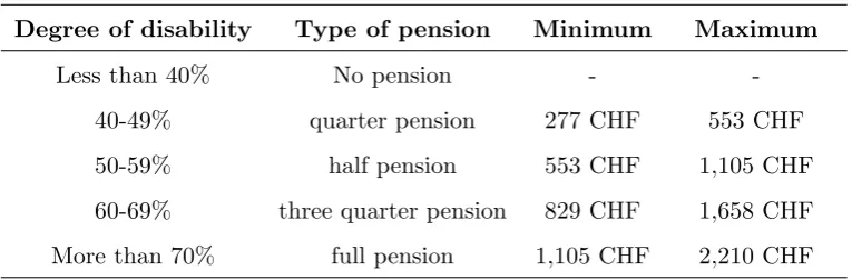
Even though the Swiss DI system emphasizes the importance of reintegration measures, examining the DI statistics presents a different picture: of the total expenditures of about 9.3 billion CHF in 2013, only 23% were spent on rehabilitation measures. The lion’s share of about 60% were used on DI pensions and helplessness allowances. A significant difference between the Swiss system and the SSDI program in the US lies in the method to calculate the amount of DI benefits. In Switzerland, the degree of disability determines the type of pension a claimant receives. The degree of disability is defined as the percentage of the loss of earnings due to disability to the potential earnings of a claimant in the absence of the impairment. Table (1) gives an overview of the types of pensions and minimum and maximum amounts associated with different degrees of disability. For example, claimants with a degree of disability less than 40% are not entitled to any pension at all, whereas claimants with a degree of disability higher than 70% are entitled to a full pension. Overall, the Swiss DI system is very generous in terms of benefits, ranking top alongside the Scandinavian countries. On the other hand, many Anglo-Saxon countries are found on the other end of the compensation rank (OECD, 2009).
— Insert Table 1 about here —
of recipients can be found among individuals aged 20-39. For this age group, job re-integration measures offered by local DI offices are primarily used. Finally, the insured in the age group below 20 years account for about 25% of all recipients. In this age segment, congenital disorders are the main cause for the DI benefit receipt (Federal Social Insurance Office, 2014).
3.2 Eligibility determination process
A person seeking benefits applies at the cantonal DI office. In a first step, the applicant sub-mits the medical documentation of his or her condition, as well as previous earnings records. Caseworkers at the local DI office in collaboration with an interdisciplinary team of medical doc-tors, specialists and vocational consultants then decide whether a person qualifies for benefits. Whether or not an applicant is eligible for benefits is based on a predefined set of medical and vocational factors such as education and age to assess a persons’ capability to work. Before the 4th revision of the Swiss DI system in 2004, the health assessment of the applicant was entirely based on the medical certificates issued by the applicant’s chosen doctor. To standardize and improve the quality of screening, the reform in 2004 introduced several supra-regional medical audit institutions that are authorized to conduct appraisals of benefit claims and to carry out medical examinations. In addition to the medical assessment, a team of vocational consultants evaluates the personal and vocational situation of the applicant. The team has to check for possible reintegration and rehabilitation measures reflecting the guiding principle rehabilitation before pension. After all the relevant information is gathered, the caseworkers have to decide on each case within 12 months. If the decision is not accepted by the applicant, appeals can be submitted to the cantonal insurance court within 30 days. Further levels of appeal are conducted in Federal Supreme Courts (Federal Social Insurance Office, 2013).
4
Data
4.1 Data source
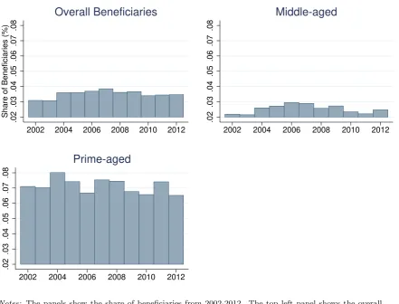
prime-aged men and women are clearly over-represented amongst the beneficiaries. On average about 7.1% of individuals between the age of 55 and 65 collect DI benefits. In the subpopulation of individuals aged 20-54 on the other hand, only about 2.5% receive benefits.
— Insert Figure 1 about here —
Second, unlike administrative datasets the SHP contains rich information on numerous back-ground characteristics that allow to isolate the effect of DI benefits on the labor supply decision of beneficiaries. The data includes information on demographic, socio-economic and various health related indicators. The demographic and socio-economic status variables include the age of the respondent at the time of the interview, an indicator for gender and dummies for region of residence6, the weight of a person in kilograms, the height of a person in centimeters, the
number of kids living in the household between the age of 0 and 17, an indicator for Non-Swiss citizens, marital status, logarithmized gross household income in Swiss Francs, years of schooling and an indicator for life satisfaction. The health indicators that we focus on in our analysis are the number of doctor consultations, the number of ill-days in the past 12 months, a physical activity indicator, an indicator for health impediments in everyday activities, an indicator for medication needed in everyday functioning, a dummy for self-assessed well-being and indicator variables for depression, anxiety and blues, back problems, weakness and weariness, sleeping problems and headaches.7
The sample is restricted to individuals between the age of 18 and 65, since there are no DI benefit recipients below and above these cutoff values. Moreover, the data cleaning procedure excludes all observations without accurate information such as filter errors, inapplicability, no answer or does not know. The final estimation sample contains 3’531 observations.
4.2 DI beneficiaries vs. non-beneficiaries
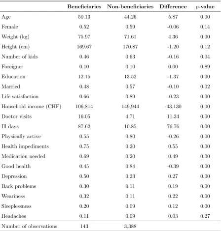
The endogeneity of benefit status can be characterized by comparing the subpopulations of DI beneficiaries and non-beneficiaries. Table (2) reports the mean values and differences in means for a selection of variables for both groups. The comparison of demographic characteristics reveals that the beneficiaries are on average older, heavier in body weight, smaller in body size and live in households with less children than the non-beneficiaries. The comparison of the socio-economic status (SES) suggests that the non-recipients are more educated than the recipients as they attend school for more than one additional year on average. In addition,
non-6
Central Switzerland is used as the base category. 7
beneficiaries typically live in households with significantly higher incomes and they are more satisfied with their life’s than the beneficiaries. Furthermore, the comparison of health indicators shows substantial differences between the groups: the beneficiaries visit the doctor about 3 times more often as the non-beneficiaries and the amount of ill-days is more than seven times as large as in the group of the non-beneficiaries. Moreover, DI benefit recipients are significantly less involved in sports activities and the share of individuals reporting a “very well” or “well” health status is about 39%-points lower for the beneficiaries. Also, around 75% of the beneficiaries claim to have health impediments that severely affect their everyday life and about 69% of them depend on medication to complete everyday tasks. As for the medical conditions, depression, anxiety and blues, back problems, weakness and weariness, sleeping problems and headaches, we find a significantly higher prevalence of such diseases in the group of beneficiaries. Overall, the data on the health indicators draws a consistent picture that suggests that the majority of those on DI benefits suffer from substantial health limitations.
— Insert Table 2 about here —
The bottom line from the mean comparisons is that the population of beneficiaries differs substantially from the population of non-beneficiaries in many observable and likely also un-observable8 characteristics. Any attempt to compare the groups with respect to their working decision is therefore doomed to fail, since we are not comparing similar groups that only differ in their benefit status. Revealing the isolated effect of DI benefits therefore at least involves con-trolling for the observable characteristics and further exploration of the underlying mechanisms that determine DI benefit status to address unobserved confounders.
5
Identification strategy
The main purpose of this study is to identify the effect of DI benefits on the labor market decision of existing DI beneficiaries. We apply a fuzzy regression discontinuity (RD) design to overcome the endogeneity issue in benefit status by exploiting a discrete jump in the benefit award rate above the age of 55. Specifically, we estimate the benefit effects on the individual decision to work part-time, full-time or stay out of the labor force using discrete endogenous switching (ES) models (Miranda & Rabe-Hesketh, 2006; Roodman, 2011).
8
5.1 Discontinuity in the benefit award rate
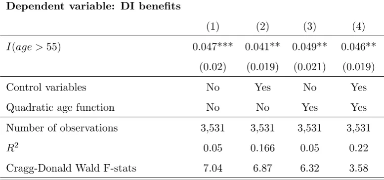
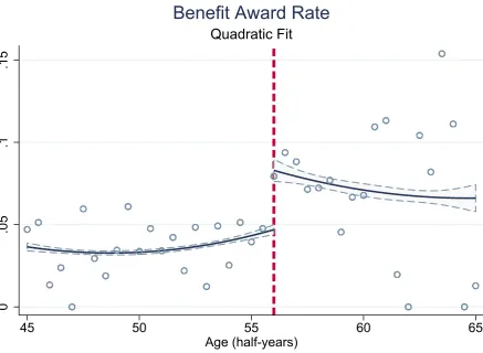
The benefit award rate is the probability of receiving DI benefits in relation to a person’s age and is depicted in Figure (2). The dots represent the mean share of beneficiaries over bins of half-years of age. The scatter plot is overlaid with a quadratic fit and a corresponding 99%-confidence interval. The dashed red vertical line indicates the age of 56. The graph shows that for the individuals below the age of 56, the benefit award rate is roughly stable at a level of about 4-5%. Above the age of 55, the probability of receiving DI benefits is well above the 5%-mark indicating a discontinuous jump in the benefit award rate at the age of 56. This means that individuals just below that age cutoff have a significantly lower probability of receiving DI benefits than people just above the discontinuity. The discontinuity is also confirmed when running classical stage regressions using the benefit status as the dependent variable. Table (3) shows the first-stage effects for four different model specifications. In all cases, the discontinuity is estimated to be approximately 4-5%-points which coincides with the graphical evidence in figure (2). The Cragg-Donald Wald F-statistics are above the usual critical values rejecting the null of a weak instrument and therefore indicating instrument relevance (Stock & Yogo, 2005).
— Insert Figure 2 and Table 3 about here —
5.2 RD validity checks
The key identifying assumption in any RD framework is based on the inability of individuals to precisely control the assignment variable near the threshold. Since applicants cannot manipulate their age, it is reasonable to assume that they have no exact control on whether they are just to the left or right of the cutoff age 56, and thus those below form a natural control group for those above. As a consequence, observable as well as unobservable characteristics should be balanced around the cutoff and treatment is “as good as randomized” (Lee & Lemieux, 2009).
To assess the validity of the RD design we check for discontinuities in the density of the forcing variable and for discontinuities in the baseline covariates at the age cutoff. Both a discontinuity in the assignment variable and predetermined variables would cast doubt on the validity of the RD design and thus our identification strategy. A common check for local random assignment is given by investigating the density of the forcing variable around the threshold. To this end, we conduct the two-step procedure proposed by McCrary (2008) and the resulting density graph can be found in Figure (3). The graph does not provide evidence for a discontinuity at the age threshold and local sorting as the confidence intervals clearly overlap.
— Insert Figure 3 about here —
As an additional validity check, we compare observable characteristics to see whether they are locally balanced around the cutoff. In fact, local random assignment implies that both observable and unobservable factors should not systematically differ between people below and above the cutoff. In Figures (4) and (5), we show the share of women and the years of schooling in a small window around the age cutoff. As clearly visible, none of the graphs indicates a statistically significant jump at the age of 56. In unreported analysis, we also looked at the pattern in some of the other variables listed in Table 2 at the age threshold. While we do not find statistically significant mean differences from just below to above the cut-off, we do not want to emphasize this result too much because some of the variables like reported health status or physical activity might be related to DI benefit status.
— Insert Figures 4 and 5 and Table 4 about here —
age 55 is systematic to the DI practice instead of an aging effect. Thus, overall, these different validity checks do not provide evidence against the RD design.
5.3 The discrete ES model
A discrete ES model is used to quantify the incentive effects of DI benefits on the working decision of existing beneficiaries. The theoretical model is derived using the framework of additive random utility models (ARUM) providing a natural connection to economic choice theory (Marschak, 1960). It is assumed that each decision maker i faces three working choices: yi ∈ {working
part-time (j= 1), full-time (j= 2), staying out of the labor force (j= 3)}. Furthermore, agents are assumed to be rationale in the sense that they choose the alternative that is associated with the highest utility for them. Utility is known by the decision maker but not by the researcher. The researcher only observes some attributes of the agent and the final working decision the individual makes (Train, 2009). The utility for individual ifrom optionj is specified as:
Uij =x′iβj +Diγj+εij ∀ j= 1,2,3; n= 1, ..., N (1)
where xi is a vector of observable characteristics, including the health indicators, demographic
and socio-economic factors described in section 4 and a flexible function in age to account for the RD setup; Di∈ {0,1} is the binary treatment indicator for DI benefit receipt;θj ≡ {βj, γj}
is the vector of model parameters with γj of main interest, andεij is an unobserved error term
that includes choice-relevant factors not contained in xi. A binary threshold crossing model is
introduced to address endogeneity of benefit status:
Di∗=wi′δ+vi (i= 1, ..., N) (2)
Di =
1 ifDi∗ >0 0 ifD∗
i ≤0
whereD∗i is a continuous random variable reflecting the latent propensity to receive DI benefits as a function of observable variables wi, which are the same as in xi but in addition include
the age cutoff as instrumental variable for the benefit status in equation (1); δ is a vector of parameters and vi an error term in the DI benefit status equation.
The vector ψi is composed of all error terms from equation (1) and (2) and is assumed to
follow a multivariate normal distribution with a mean vector of zero and covariance matrix Ω:
ψi=
εi1
εi2 εi3
vi
∼ MVN(0,Ω) where Ω =
σ12 σ12 σ13 σ1v
· σ22 σ23 σ2v
· · σ32 σ3v
· · · σ2v
To ensure parameter identification, one needs to acknowledge that the level and scale of the latent utilities are irrelevant in the model. The absolute level of utility is irrelevant because adding any constant c to the utility of each working option does not change the ordering of utilities and therefore has no effect on the observed labor supply choice of the beneficiary. The level of utility is normalized by choosing a base category (we will use part-time as the base throughout the analysis) and setting the corresponding parameter vector to zero, i.e., θ1= 0. Similarly, the
scale is irrelevant because each latent utility can be multiplied by a positive constant cwithout changing which alternative has the highest utility (Train, 2009). The scale is normalized by imposing constraints on Ω as discussed in Bunch (1991) and Roodman (2011)9.
5.4 Simulation of choice probabilities
Using the structural form of the model, probabilistic statements about individual work decisions can be made. For example, the probability of working full-time given DI benefits is given by:
P(yi = 2|Di = 1, xi) =
P(Ui2> Ui1, Ui2 > Ui3, Di∗ >0)
P(D∗
i >0)
(4)
=
Z x′iβ2+Diγ2
−∞
Z x′i(β2−β3)+Di(γ2−γ3)
−∞
φ2(˜ε12,ε˜32)dε˜12dε˜32
− Rx′iβ2
−∞
Rx′i(β2−β3)
−∞
R−wiδ
−∞ φ3(˜ε12,ε˜32, vi)dε˜12dε˜32dvi
Φ(−wiδ)
= Φ2(x′iβ2+Diγ2, x′i(β2−β3) +Di(γ2−γ3);V1)
−Φ3(x ′
iβ2, x′i(β2−β3),−wiδ;V)
Φ(−wiδ)
where φ2(·) and φ3(·) are bi- and trivariate standard normal densities, Φ2(·) and Φ3(·) are
the corresponding bi- and trivariate standard normal cdf’s with correlation matrix V of the differenced errors ˜εjk =εj −εk in the utility equations for options j and k, andV1 ≡ρ˜ε12,˜ε23 is
the correlation between ˜ε12 and ˜ε23. Equation (4) demonstrates that the choice probabilities in
the discrete ES model are multivariate integrals over subsets of the Euclidean space. The problem is that these choice probabilities cannot be expressed in closed-form. Instead, one has to use simulation methods to evaluate the integrals numerically. We use the Geweke, Hajivassiliou and Keane (GHK) algorithm (Geweke, 1991; Hajivassiliou & McFadden, 1998; Keane, 1990 & 1994a), which has been shown to simulate normal probabilities well (Hajivassiliou et al. 1994). The GHK-algorithm is based on the idea that the choice probabilities in (4) can be re-expressed as a sequence of conditional probabilities that can be simulated recursively. The basic principle of the
9
We follow the standard approach in the literature by imposing variance unity on the error terms to normalize
algorithm is to take a predefined number of draws from the unit interval for each observation and to generate the simulated probability at each iteration step. In this paper, we use the GHK-based conditional mixed process estimator as it is programmed in the Stata routine cmp provided by Roodman (2011). The latent model parameters are estimated by maximum simulated likelihood (MSL), the corresponding log-likelihood function can be found in Appendix A.2.
5.5 Treatment effects
To illustrate the DI benefit effects, we use the latent model coefficients to derive the treatment effect on treated for each labor market outcome. To give an example, the treatment effect on the treated (TOT) for the outcome of working full-time is given by
T OTf ull = P(yi1= 2|Di= 1, xi)−P(yi0 = 2|Di= 1, xi) (5)
= Φ2(x′iβ2+Diγ2, x′i(β2−β3) +Di(γ2−γ3);V1)−Φ2(x′iβ2, x′i(β2−β3);V1)
and similarly for the TOT of working part-time and being out of the labor force. The TOT re-flects the difference between the probability of working full-time given that beneficiaryireceived DI benefits and the probability of working full-time given that the exact same beneficiary did not receive benefits. A negative TOT therefore indicates that the DI benefit receipt decreases the probability of working full-time and vice versa for a positive TOT.
6
Results
6.1 DI benefit effects for the average beneficiary
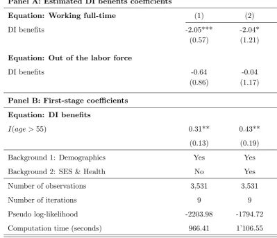
Table (5) shows the estimated coefficients of the discrete ES model for two different model specifications. The table is constructed such that the upper panel shows the estimated utility parameters on the DI benefits for the labor market outcomes of working full-time and staying out of the labor force, whereas the lower panel shows the estimated parameter on the instrument. In both models, the discontinuity in the benefit award rate above the age of 55 is used as the instrument for the benefit status and working part-time is used as the baseline category. In a first step, we estimate the benefit effects while controlling exclusively for demographic background characteristics10. As a result, we obtain a highly significant and negative coefficient
on the benefit status regarding the decision of working full-time. At the same time, there is no statistically significant effect of the DI benefits on the decision of staying out of the labor force.
— Insert Table 5 about here —
In a second step, we add control variables for socio-economic background11, as well as
in-dividual health status12 to our model. Again, we find a negative coefficient on DI benefits for the decision of working full-time but less significant. On the other hand, the coefficient on the benefits for the outcome of not working is close to zero and still far from statistically significant. In addition, our discrete ES model also produces a highly significant first-stage effect which is of same magnitude as shown in Table (3).13 Note that the coefficient estimates in the second specification are basically unchanged if further control variables are added to the equation, like health indicators (number of hospital days, number of specialist visits) and parental education as a proxy for genetic endowment, reinforcing the robustness of the presented findings.
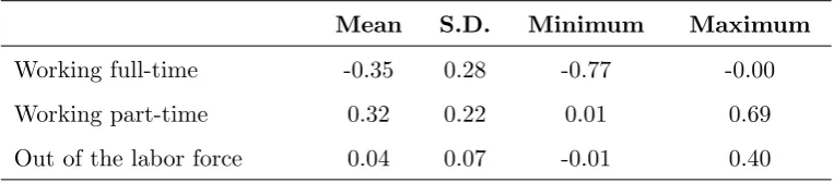
The fact that the coefficient on the benefit status for the labor market outcome of working full-time is negative and significant in all specifications suggests, at first glance, that the DI benefits provide strong work disincentives for the existing beneficiaries. However, to appropri-ately address the question on the benefit effects on the labor market decision of beneficiaries, one needs to translate coefficients into treatment effects as outlined in the previous section. The treatment effects on the treated (TOT) provide the relevant information on the changes in the labor supply decision of an existing beneficiary to the working decision of the same person in the absence of the DI benefits (the counterfactual). Table (6) gives the relevant summary statistics
10
Age, gender, weight, height, number of kids, foreigner and region dummies (base: Central Switzerland) 11
Marital status, years of schooling, log household income, life satisfaction 12
Number of doctor visits, ill-days, physical activity, health impediments, medication needed, indication for self-assessed health and dummies for depression, back problems, weariness, headaches, sleeping problems.
13
of the TOT for each labor market outcome. Starting with the discussion on the benefit effects for the decision of working part-time, we see that for the average beneficiary the probability of working part-time is increased by about 32%-points. In other words, the probability of working part-time for the average beneficiary would have been about 32%-points lower in the absence of DI benefits. Conditional on health status, demographic and socio-economic background of a beneficiary, the results provide strong evidence that the decision of working part-time is signifi-cantly influenced by the benefit status. The treatment effects are strictly positive ranging from roughly 0%-points to a maximum of about 69%-points, which indicates that the probability of working part-time is increased for all beneficiaries in the sample.
Exactly opposite to the effect on the probability of working part-time, we find that a DI benefit receipt on average decreases the probability of working full-time by about 35%-points. Hence the probability of working full-time would have been about 35%-points higher for the average beneficiary if he/she was not entitled to DI benefits. Furthermore, we see that the treatment effects are strictly negative and range from about 0%-points to roughly -77%-points, indicating that the benefit receipt in general decreases the probability of working in a full-time job. Taken together, this leads to the conclusion that DI benefits induce existing beneficiaries to shift their work intensity from full-time to part-time. Following that line of thinking, the financial incentives provided by the Swiss DI system create substantial lock-in effects which at least in part might explain the low DI outflow of existing beneficiaries.
What remains is the discussion of the DI benefit effects for the labor market outcome of being out of the labor force. Table (6) shows that the probability of being out of the labor force is only weakly increased by about 4%-points for the average beneficiary. However, there is substantial heterogeneity in the effects, with some beneficiaries affect by as much as +40%-points. This heterogeneity will be further analyzed in the next subsection.
To summarize, the average beneficiary tends to shift work intensity from full- to part-time, and the probability of dropping out of the labor force is hardly influenced by the DI benefits. The analysis of this more complex labor market decision reveals aspects which have not been captured by the literature before, which has mainly focused on the simple binary working decisions (e.g. Bound (1989), Gruber (2000), Chen and van der Klaauw (2008), Marie and Vall Castello (2012)).
6.2 Effect Heterogeneity
outcomes separately plus the corresponding quartiles dividing the distributions into four equally-sized groups of beneficiaries. Regarding the decision of working part-time, Figure (6) provides two key insights. First, the TOTs are all non-negative indicating that a DI benefit receipt increases the probability of working part-time for all beneficiaries in the sample. Second, the TOTs range from 0%-points to a maximum of 69%-points, which suggests substantial effect heterogeneity between DI beneficiaries. In fact, the lower quartile of the TOTs ranges from 0%-points to 12.6%-points suggesting rather small reactions in the labor supply decision as a response to benefit receipt. On the other hand, beneficiaries in the upper quartile heavily respond to the benefits as the likelihood of working part-time is increased by about 53%-points up to 68%-points.
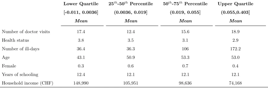
Based on this evidence for effect heterogeneity, the question arises how the members of the different quartiles can be characterized. Table (7) gives an answer to this question showing the mean values for a selection of health, demographic and socio-economic status variables for each of the quartiles. When comparing the beneficiaries in the highest quartile with the strongest reaction to the benefits to those in the lowest quartile with the weakest reaction, then three major differences between the groups can be identified. The reaction to the DI benefits is strongest for (i) men, who are in (ii) relatively good health as indicated by the lowest number of doctor visits and number of ill-days and who have (iii) relatively high incomes. The fact that especially those beneficiaries with low-income react the least to the benefits can be explained by the comparably high replacement rate of benefits for those individuals. In addition, being in poor health might explain a general inability to adjust the individual labor supply.
— Insert Figures 6, 7 and 8 and Table 7 about here —
Moving on to the discussion of working full-time, Figure (7) shows that the TOTs are weakly negative for all beneficiaries. The probability of working full-time for beneficiaries in the lowest quartile of the TOT distribution is reduced between 67%-points and 77%-points. In contrast, for beneficiaries in the upper quartile the probability to work full-time is reduced between 0%-points and 9%-points. Again it is interesting to compare the beneficiaries in the different quartiles regarding their observable characteristics (see Table (7)). The beneficiaries in the lower quartile with a strong negative reaction to DI benefits are mostly men with a comparably high socio-economic status who are in relatively good health. Combining these results leads to the conclusion that especially comparatively healthy men with high income adjust their labor supply from working full-time to part-time as a response to DI benefit receipt.
of the labor force has highest mass around small positive effects, but the upper quartile of the distribution indicates effects of DI benefits from 5.5 to 40.3%-points. Consistent with the above results, Table (7) indicates that it is mainly the low-income individuals and the beneficiaries in bad health that drop out of the labor market.
6.3 Additional sensitivity checks
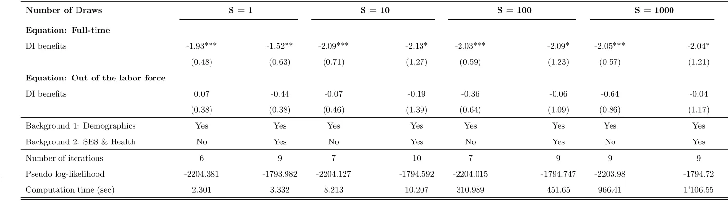
In this section, we show the estimated model coefficients as the number of pseudo-random draws (S) increases. Table (8) shows the discrete ES estimates for 1, 10, 100 and 1000 draws per observation, the number of iterations needed to reach convergence, the value of the pseudo log-likelihood at the coefficient vector and the computation time in seconds. All simulations were ran on an Intel(R) Core(TM) i7-4790 CPU @ 3.60 GHz with 16GB RAM on Windows 10 using Stata/MP 14.0. Recall that the main results are based on 1000 draws per observation so that Table (8), column 4 is identical to the results presented earlier. For small numbers of draws, we know from asymptotic theory that the MSL estimator is not equivalent to the ML estimator and is inconsistent (Gouri´eroux & Monfort, 1991). This is likely to be the case for the estimates corresponding to S = 1 and S = 10 draws per observation. For such small S, the significantly reduced computation time comes at the cost of inconsistent parameter estimates. However, as the number of draws is increased to S= 100 or higher, the MSL estimates stabilize and remain basically unchanged. Table (8) suggests that estimates with as few as 100 random draws per observation produce reliable coefficient estimates that are close to those withS = 1000. This is also relevant to know from a practical point of view since the differences in computation time are considerable: for the full specification used to produce the results discussed in the last section, the computation time is roughly 7 minutes for S = 100, but already 18 minutes for S = 1000. If the number of draws is further increased above S = 100014, the coefficient estimates hardly change but again come at the cost of a much higher computational time.
7
Concluding remarks
Over the course of the past few decades, the number of beneficiaries and the costs of DI programs have exploded in most OECD countries. At the same time only a small fraction of those who are entitled to DI benefits ever leave the DI system and very little is known about the mechanisms related to DI outflow. Policy-makers who want to effectively improve the incentive structure of the DI system therefore need to ask the question of how the working decision of existing
14
beneficiaries is affected by the DI benefits. This paper investigates this question by analyzing the potential lock-in effects created by the financial incentives embodied in the Swiss DI system. We use a fuzzy RD design exploiting a discontinuity in the DI benefit award rate to instru-ment individual benefit status. Allowing for a multinomial outcome of labor force participation (full-time, part-time, out of the labor force), we estimate discrete endogenous switching (ES) models (Miranda & Rabe-Hesketh, 2006; Roodman, 2011) to identify the benefit effects on the labor market decision of existing beneficiaries. Unlike the existing literature (e.g. Gruber (2000), Chen & van der Klaauw (2008), Marie & Castello (2012), French & Song (2014), Moore (2015)), we do not confine ourselves on the binary choice of working versus not working. The main reason for this choice is that we expect stronger effects at the intensive than the extensive margin due to the principle in the Swiss DI system of rehabilitation before pension.
Our results reveal important new aspects of the labor supply decision of existing beneficiaries and confirm earlier evidence that individual working decisions are considerably influenced by DI benefits. The DI benefits, conditional on demographic and socio-economic background and health status, increase the probability of working in a part-time employment by about 32%-points, decrease the probability of working full-time by about 35%-points and have little or no effect on the decision of staying out of the labor force for the average beneficiary. It follows that the DI benefits induce a change in the labor supply of beneficiaries from working full-time to working part-time instead of forcing them completely out of the labor market. A positive interpretation of these findings would be that the DI system works in the sense that people who receive benefits remain in the work force. A more critical interpretation is that the financial incentives provided by the DI system triggers beneficiaries to lower their work intensity and therefore keeps them dependent on income transfers, which in turn adds a possible explanation for the low DI outflow.
Appendix A1
Variable construction
The indicator for DI benefits is constructed from a question about the annual amount of DI pensions a person receives and equals one for individuals who report to receive DI benefits and zero for those who do not receive income transfers from the Swiss DI. There is also information about the amount of DI pensions in the Swiss Household Panel, but we decided against using this variable as the main explanatory variable in our model because of many missing values and likely reporting error, which would yield biased results. The discrete labor force participation variable is equal to 1 for individuals who work part-time, it is equal to 2 for those who work full-time and equal to 3 for those who are unemployed or not in the labor force.
Appendix A2
Simulated log-likelihood
The vector of model parameters θj ≡ {βj, γj} and Ω are estimated by maximizing a simulated
log-likelihood function of the form,
SLL(θ,Ω;x, y) =
3
X
j=1
N
X
n=1
dijDilog( ˜P(yi=j|Di = 1))
+
3
X
j=1
N
X
n=1
dij(1−Di) log( ˜P(yi=j|Di= 0)) (6)
where dij is an indicator for the choice taken by individual i, Di is the indicator for the DI
Tables and Figures
Table 1: Degree of disability and pensions
Degree of disability Type of pension Minimum Maximum
Less than 40% No pension - -40-49% quarter pension 277 CHF 553 CHF 50-59% half pension 553 CHF 1,105 CHF 60-69% three quarter pension 829 CHF 1,658 CHF More than 70% full pension 1,105 CHF 2,210 CHF
Source:Federal Social Insurance Office (2014). Notes: The minimum and maximum pensions
Table 2: Mean comparison of beneficiaries and non-beneficiaries
Beneficiaries Non-beneficiaries Difference p-value
Age 50.13 44.26 5.87 0.00
Female 0.52 0.59 -0.06 0.14 Weight (kg) 75.97 71.61 4.36 0.00 Height (cm) 169.67 170.87 -1.20 0.12 Number of kids 0.46 0.63 -0.16 0.04 Foreigner 0.10 0.10 0.00 0.89 Education 12.15 13.52 -1.37 0.00 Married 0.48 0.57 -0.10 0.02 Life satisfaction 0.66 0.89 -0.23 0.00 Household income (CHF) 106,814 149,944 -43,130 0.00 Doctor visits 16.05 4.71 11.34 0.00 Ill days 87.62 10.85 76.76 0.00 Physically active 0.55 0.80 -0.26 0.00 Health impediments 0.75 0.20 0.55 0.00 Medication needed 0.69 0.20 0.49 0.00 Good health 0.45 0.84 -0.39 0.00 Depression 0.50 0.23 0.27 0.00 Back problems 0.30 0.11 0.19 0.00 Weariness 0.32 0.11 0.22 0.00 Sleeplessness 0.20 0.09 0.12 0.00 Headaches 0.11 0.09 0.03 0.27 Number of observations 143 3,388
Table 3: First-stage regression of DI benefit receipt on age threshold
Dependent variable: DI benefits
(1) (2) (3) (4)
I(age >55) 0.047*** 0.041** 0.049** 0.046**
(0.02) (0.019) (0.021) (0.019) Control variables No Yes No Yes Quadratic age function No No Yes Yes Number of observations 3,531 3,531 3,531 3,531
R2 0.05 0.166 0.05 0.22 Cragg-Donald Wald F-stats 7.04 6.87 6.32 3.58
Notes: First-stage regression results using the indicator for DI benefits as dependent variable
and data in a window of±20 years around the age cutoff. The instrumental variable is the
indicator for the discontinuity in the benefit award rate above the age of 55. All specifications
include age centered around threshold and an interaction of centered age and the instrument.
The set of exogenous controls variables includes all the demographic, socio-economic and health
related variables as described in Section 4. Standard errors are clustered at the household level.
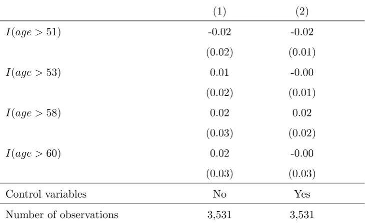
Table 4: Testing alternative cutoffs
Dependent variable: DI benefits
(1) (2)
I(age >51) -0.02 -0.02
(0.02) (0.01)
I(age >53) 0.01 -0.00
(0.02) (0.01)
I(age >58) 0.02 0.02
(0.03) (0.02)
I(age >60) 0.02 -0.00
(0.03) (0.03) Control variables No Yes Number of observations 3,531 3,531
Notes:First-stage regression results using the indicator for DI benefits as dependent
vari-able and data in a window of±20 years around the age cutoff. All specifications include
age centered around threshold and an interaction of centered age and the instrument.
The set of exogenous controls variables includes all the demographic, socio-economic
and health related variables as described in Section 4. Standard errors clustered at the
Table 5: Discrete ES estimates of the effect of DI benefits on labor supply
Panel A: Estimated DI benefits coefficients
Equation: Working full-time (1) (2)
DI benefits -2.05*** -2.04* (0.57) (1.21)
Equation: Out of the labor force
DI benefits -0.64 -0.04 (0.86) (1.17)
Panel B: First-stage coefficients
Equation: DI benefits
I(age >55) 0.31** 0.43**
(0.13) (0.19) Background 1: Demographics Yes Yes Background 2: SES & Health No Yes Number of observations 3,531 3,531 Number of iterations 9 9 Pseudo log-likelihood -2203.98 -1794.72 Computation time (seconds) 966.41 1’106.55
Notes: Discrete ES coefficient estimates on the DI benefit status for the labor market outcomes
of working full-time and out of the labor force (base category: working part-time) based on
1’000 antithetic GHK draws. Coefficients on background variables not shown. Standard errors
clustered at the household level. Significance levels: ***p <0.01 **p <0.05 *p <0.1.
Background 1: Age, gender, weight (kg), height (cm), number of kids, foreigner, region dummies
(base: Central Switzerland), type of community dummies (base: rural)
Background 2: Marital status, years of schooling, logarithmized household income, life
satisfac-tion, number of doctor visits, number of ill-days, physical activity, health impediments,
medi-cation needed, indimedi-cation for self-assessed health and dummies for depression, back problems,
Table 6: Average effects of DI benefits derived from discrete ES model
Mean S.D. Minimum Maximum
Working full-time -0.35 0.28 -0.77 -0.00 Working part-time 0.32 0.22 0.01 0.69 Out of the labor force 0.04 0.07 -0.01 0.40
Notes: Summary statistics of the TOTs for the labor market outcomes working full-time,
part-time and out of the labor force. The TOTs are based on the coefficient estimates from
Table 7: Mean values of background characteristics by TOT quartile
Working full-time
Lower Quartile 25th-50thPercentile 50th-75thPercentile Upper Quartile
[-0.768, -0.674] (-0.674, -0.283] (-0.283, -0.090] (-0.090, -0.000]
Mean Mean Mean Mean
Number of doctor visits 13.5 14.4 8.8 27.9
Health status 3.2 3.5 3.6 3.0
Number of ill-days 121.3 65.9 51.9 112.5
Age 53.2 47.7 45.9 53.9
Female 0.0 0.3 0.8 1.0
Years of schooling 12.8 12.5 11.5 11.8
Household income (CHF) 111,765 111,696 113,423 89,849
Working part-time
Lower Quartile 25th-50thPercentile 50th-75thPercentile Upper Quartile
[0.009, 0.126] (0.126, 0.268] (0.268, 0.524] (0.524, 0.686]
Mean Mean Mean Mean
Number of doctor visits 26.4 10.9 11.8 15.0
Health status 3.0 3.5 3.3 3.5
Number of ill-days 100.7 86.1 91.4 71.8
Age 52.6 47.3 47.8 52.9
Female 0.9 0.7 0.4 0.1
Years of schooling 11.8 11.6 12.3 12.9
Household income (CHF) 100,841 97,861 101,428 112,770
Out of the labor force
Lower Quartile 25th-50thPercentile 50th-75thPercentile Upper Quartile
[-0.011, 0.0036] (0.0036, 0.019] (0.019, 0.055] (0.055,0.403]
Mean Mean Mean Mean
Number of doctor visits 17.4 12.4 15.6 18.9
Health status 3.8 3.5 3.1 2.9
Number of ill-days 36.4 36.3 106 172.2
Age 43.1 50.9 53.3 53.0
Female 0.3 0.6 0.7 0.4
Years of schooling 12.4 12.1 12.1 12.1
Household income (CHF) 148,990 105,951 98,636 74,168
Table 8: Sensitivity checks on the number of simulation draws
Number of Draws S = 1 S = 10 S = 100 S = 1000
Equation: Full-time
DI benefits -1.93*** -1.52** -2.09*** -2.13* -2.03*** -2.09* -2.05*** -2.04*
(0.48) (0.63) (0.71) (1.27) (0.59) (1.23) (0.57) (1.21)
Equation: Out of the labor force
DI benefits 0.07 -0.44 -0.07 -0.19 -0.36 -0.06 -0.64 -0.04
(0.38) (0.38) (0.46) (1.39) (0.64) (1.09) (0.86) (1.17)
Background 1: Demographics Yes Yes Yes Yes Yes Yes Yes Yes
Background 2: SES & Health No Yes No Yes No Yes No Yes
Number of iterations 6 9 7 10 7 9 9 9
Pseudo log-likelihood -2204.381 -1793.982 -2204.127 -1794.592 -2204.015 -1794.747 -2203.98 -1794.72
Computation time (sec) 2.301 3.332 8.213 10.207 310.989 451.65 966.41 1’106.55
Notes:Discrete ES coefficient estimates using different numbers of simulation draws (S). The simulations were ran on an Intel(R) Core(TM) i7-4790 CPU @ 3.60 GHz with 16GB RAM on Windows 10 using
Stata/MP 14.0. See notes from table (6) for a description of the background characteristics used in each specification. Standard errors clustered at the household level: ***p <0.01 **p <0.05 *p <0.1.
Figure 1: Share of DI beneficiaries
.02
.03
.04
.05
.06
.07
.08
Share of Beneficiaries (%)
2002 2004 2006 2008 2010 2012
Overall Beneficiaries
.02
.03
.04
.05
.06
.07
.08
2002 2004 2006 2008 2010 2012
Middle-aged
.02
.03
.04
.05
.06
.07
.08
2002 2004 2006 2008 2010 2012
Prime-aged
Notes: The panels show the share of beneficiaries from 2002-2012. The top left panel shows the overall
share of beneficiaries which is at a level of about 3.5% within this timeframe. The top right panel shows
the share of beneficiaries for the middle-aged (ages 20-54) subpopulation (average: 2.5%). The bottom left
panel finally shows the percentage of DI beneficiaries between the ages of 55-65 with an average share of
Figure 2: RD validity checks I: discontinuity in the benefit award rate
0
.05
.1
.15
45 50 55 60 65
Age (half-years)
Quadratic Fit
Benefit Award Rate
Notes: The figure displays the discontinuity in the benefit award rate overlaid with a quadratic fit and the
Figure 3: RD validity checks III: density of the forcing variable
0
.01
.02
.03
.04
0 20 40 60 80
Notes: The figure displays the years of schooling around the age cutoff at 56 (bins of half-years of
Figure 4: RD validity checks II: inspection of baseline covariates
.4
.45
.5
.55
.6
.65
45 50 55 60 65
Age (half-years) Linear Fit
Share of Women
Notes: The figure displays the discontinuity in the benefit award rate overlaid with a quadratic fit
Figure 5: RD validity checks II (cont’d): inspection of baseline covariates
12.
5
13
13.
5
14
14.
5
45 50 55 60 65
Age (half-years) Linear Fit
Years of Schooling
Notes: The figure displays the share of women around the age cutoff at 56 (bins of half-years of
Figure 6: Distribution of the treatment effects on the treated (TOT), part I
Average TOT: 32-ppts
Lower Quartile Median Upper Quartile
0
2
4
6
Share
of
B
enef
iciaries
(%)
0 .1 .2 .3 .4 .5 .6 .7
Treatment effect on treated (%-points)
Working Part-Time
Notes: The figure shows the distribution of the treatment effect on treated (TOT) for the labor market
outcome of working part-time overlaid with a kernel density estimate. The dashed lines indicate the 25th,
the 50th and the 75th percentiles. A positive (negative) sign on the TOT indicates an increase (decrease)
Figure 7: Distribution of the treatment effects on the treated (TOT), part II
Average TOT: -35-ppts
Lower Quartile Median Upper Quartile
0
5
10
Share
of
B
enef
iciaries
(%)
-.8 -.6 -.4 -.2 0
Treatment effect on treated (%-points)
Working Full-Time
Notes: The figure shows the distribution of the treatment effect on treated (TOT) for the labor market
outcome of working full-time overlaid with a kernel density estimate. The dashed lines indicate the 25th,
the 50th and the 75th percentiles. A positive (negative) sign on the TOT indicates an increase (decrease)
in the probability of working full-time as a response to the benefit receipt.
References
Angrist, J. D. & Pischke, J.-S. (2009), Mostly Harmless Econometrics – An Empiricist’s Companion, Princeton University Press.
Autor, D. H. & Duggan, M. G. (2003), The Rise in Disability Rolls and the Decline in Unemployment, The Quarterly Journal of Economics, vol. 118 (1), 157-205.
Bhat, C.(2001), Quasi-random maximum simulated likelihood estimation of the mixed multi-nomial logit model, Transportation Research, B 35, 677-693.
Figure 8: Distribution of the treatment effects on the treated (TOT), part III
Average TOT: 4%-ppts Lower Quartile
Median
Upper Quartile
0
10
20
30
Share
of
B
enef
iciaries
(%)
0 .1 .2 .3 .4
Treatment effect on treated (%-points)
Out of the Labor Force
Notes: The figure shows the distribution of the treatment effect on treated (TOT) for the labor market
outcome of staying out of the labor force overlaid with a kernel density estimate. The dashed lines indicate
the 25th, the 50th and the 75th percentiles. A positive (negative) sign on the TOT indicates an increase
(decrease) in the probability of staying out of the labor market as a response to the benefit receipt.
Bound, J. & Burkhauser, R. V. (1999), Economic analysis of transfer programs targeted on people with disabilities. In: Ashenfelter, O., Card, D. (Eds.), Handbook of Labor Economics, vol. 3C. North-Holland, Amsterdam.
Burkhauser, R. V., Daly M. C., McVicar D., Wilkins R. (2013), Disability Benefit Growth and Disability Reform in the U.S.: Lessons from Other OECD Nations, Federal Reserve Bank of San Francisco, Working Paper Series.
Bunch, D. (1991), Estimability in the multinomial probit model, Transportation research, B 25, 1-12.