Fitted ROC Model Parameters
MWITONDI, Kassim, MOUSTAFA, R E and HADI, A S
Available from Sheffield Hallam University Research Archive (SHURA) at:
http://shura.shu.ac.uk/9389/
This document is the author deposited version. You are advised to consult the
publisher's version if you wish to cite from it.
Published version
MWITONDI, Kassim, MOUSTAFA, R E and HADI, A S (2013). A Data-Driven Method
for Selecting Optimal Models Based on Graphical Visualisation of Differences in
Sequentially Fitted ROC Model Parameters. Data Science Journal, 12,
WDS247-WDS253.
Copyright and re-use policy
See
http://shura.shu.ac.uk/information.html
A DATA-DRIVEN METHOD FOR SELECTING OPTIMAL MODELS
BASED ON GRAPHICAL VISUALISATION OF DIFFERENCES IN
SEQUENTIALLY FITTED ROC MODEL PARAMETERS
K S Mwitondi*
1, R E Moustafa
2, and A S Hadi
3*1Sheffield Hallam University, Faculty of Arts, Computing, Engineering and Sciences, Sheffield S1 1WB, UK
Email: [email protected]
,
[email protected]2George Washington University, Statistics Department, 2140 Pennsylvania Ave., NW, Washington DC, 20052,
USA
Email: [email protected]
,
[email protected]3The American University in Cairo, Egypt/Cornell University, 291 Ives Hall, Cornell University, Ithaca, NY
14853-3901, USA
Email: [email protected]
,
[email protected]ABSTRACT
Differences in modelling techniques and model performance assessments typically impinge on the quality of knowledge extraction from data. We propose an algorithm for determining optimal patterns in data by separately training and testing three decision tree models in the Pima Indians Diabetes and the Bupa Liver Disorders datasets. Model performance is assessed using ROC curves and the Youden Index. Moving differences between sequential fitted parameters are then extracted, and their respective probability density estimations are used to track their variability using an iterative graphical data visualisation technique developed for this purpose. Our results show that the proposed strategy separates the groups more robustly than the plain ROC/Youden approach, eliminates obscurity, and minimizes over-fitting. Further, the algorithm can easily be understood by non-specialists and demonstrates multi-disciplinary compliance.
Keywords: Bayesian error, Data mining, Data visualisation, Decision trees, Domain partitioning, Optimal bandwidth, ROC curves, Visual analytics, Youden Index
1
INTRODUCTION
Choosing from a range of competing models is a common practice in predictive modelling in which the selection of the optimal model and its performance depends on a combination of factors. In classification, for instance, the consequences of misclassification largely depend on the true class of the object being classified and the way it is ultimately labelled. Generally, the performance of both parametric and non-parametric models depends exclusively on the chosen model, the sampled data, and the available knowledge for the underlying problem. For instance, the accuracy and reliability of, say, a medical test will depend not only on the diagnostic tools but also on the definition of the state of the condition being tested. Such variations make model complexity a natural challenge to data modelling (Mwitondi, 2010). Thus, when data sources, repositories, and modelling tools are shared, it is imperative to work out a unifying environment with the potential to yield consistent results across applications. Achieving this goal requires striking a balance between model accuracy and reliability across applications (Mwitondi & Said, 2011). This paper examines how multiple model performances can be used to devise a generalised strategy for attaining the foregoing balance in predictive modelling. Using a generic two-class scenario, it addresses the underlying issues relating to prediction errors and combines model generated numerals and graphics to decipher data patterns for optimality. More specifically, the paper sets off from conventional approaches for group separation, ROC curves (Egan, 1975) and the Youden Index (Youden, 1950), to propose an iterative algorithm for detecting separation levels based on estimated data densities. The paper is organised as follows. Section 2 provides an overview of the methods and simulations. Section 3 outlines the modelling strategy, implementation, results, and discussions. The concluding remarks and potential future applications are outlined in Section 4.
2
METHODS AND SIMULATIONS
The ultimate goals are to illustrate the nature of variation in the performance of various models given the random nature of the data used to train and test them and to devise a modelling strategy for optimising the model selection process. The illustrations and the strategy derive from the Bayesian rule as outlined in Berger (1985), the decision trees (DT) domain partitioning technique as described in Breiman et al. (1984), and the receiver operating characteristics (ROC) analysis as outlined in Egan (1975).
2.1 Allocation rule errors due to data randomness
As shown in Table 1, the total empirical error is typically associated with randomness due to the allocation region and randomness due to assessing the rule by random training and validation data (Mwitondi, 2003). Table 1. Error types associated with domain-partitioning modelling (Source: Mwitondi, 2003)
POPULATION TRAINING CROSS VALIDATION TEST
Thus, given that there are data points in different classes, the overall misclassification error is computed as the sum of the weighted probabilities of observing data belonging to a particular class given that we are not in that class. For instance,
∑ ∑ ( ) ( ) (1)
where and ( ) represent the partition region and the class priors respectively in a typical Bayesian context. Various approaches for minimising this error have been proposed - see, for instance, Reilly and Patino-Leal (1981), Wan (1990), Freund and Schapire (1997), and Mwitondi et al. (2002). A commonly acceptable practice is to vary the allocation rule in order to address specific requirements of an application. We illustrate the scenario based on decision trees as in Breiman et al. (1984) and ROC curves (Egan, 1975).
2.2 Decision trees modelling
Growing a tree amounts to sequentially splitting the data into, typically, two super sets, A and B, based on a single predictor at a time. The observations in A and B lie on either side of the hyper-plane chosen in such a way that a given measure of impurity is minimised. The splitting continues until an adopted stopping criterion is reached. Selecting an optimal model is one of the major challenges data scientists face. Breiman et al. (1984) propose an automated cost-complexity measure described as follows. Let the complexity of any sub-tree be defined by its number of terminal nodes, . Then, if we define the cost-complexity parameter , the cost-complexity measure can be defined as
( ) ( ) (2)
Let be any branch of the sub-tree ( ), and define ( ) ∑ ( )
where represents the set of all terminal nodes in . They further show that given t any non-terminal node in ( ), the inequality ( )
( ) holds. It can be shown that for any sub-tree we can define a measure impurity as a function of as
( ) ( ) (3)
2.3 ROC curves analysis, optimality, and Youden Indexing
Without loss of generality, consider a binary medical diagnostic test scenario in which patients are tested for a particular disease and there are four possible outcomes: true positive (TP), true negative (TN), false positive (FP), and false negative (FN). In this case, the ROC curve is constructed based on the proportions
(4)
where SST and SPT denote the sensitivity and specificity respectively and NTP and NFN denote
the number of those with the disease and who are diagnosed with it and those having the disease but cleared by the test respectively. Similarly, NTN and NFP are the number of those without the disease who test negative and
those testing positive without having the disease, respectively. As with type I and II errors, the usefulness of a test cannot be determined by SST/SPT alone, and so a ROC analysis trade-off is needed. Assuming four possible outcomes, the ROC accuracy (ACCR) and error (ERR) are defined as
(5)
If we denote the data by X and the set of class labels as { }, the probability of accuracy can be
computed as follows, where the integral is over both classes.
( ) ( ) ∑ ( )∫ ( ) ( ) ( ) (6)
The main goal of predictive modelling is to maximise ( ) or equivalently minimise ( ) consistently across applications. By appropriately costing each of the class allocation measures, we can make the outcome not only depend on the diagnostic tools and techniques but also on the definition of the state of the tested condition. For instance, one would rather set “low specificity” for a cancer diagnostic test, i.e., let it trigger on low-risk symptoms, than miss the symptoms. Our model implementations are focused on striking this balance. One way of determining the optimal cut-off point for the ROC curves is to use the Youden Index (Youden, 1950). Its main idea is that for any binary classification model with corresponding cumulative distribution functions ( ) and ( ), say, then for any threshold t, the relationship ( ) ( ) ( ) ( )
holds. We can then compute the index as the maximum difference between the two as
{ ( ) ( ) } { ( ) ( )} (7)
Within a model, the Youden Index is the maximum differences between the true and false positive values and between competing models ordering of the indices highlights performance order.
3
MODELLING STRATEGY, IMPLEMENTATION, RESULTS, AND
DISCUSSIONS
Table 2. Data attributes for the Pima Indians diabetes and the Bupa liver disorders datasets
PIMA INDIANS DIBETES DATA BUPA LIVER DISORDERS DATA
NTP Number of times pregnant MCV Mean corpuscular volume
PGC Plasma glucose concentration ALKPHOS Alkaline phosphotase
DBP Diastolic blood pressure SGPT Alamine aminotransferase
TSF Triceps skin fold thickness SGOT Aspartate aminotransferase
BMI Body mass index GAMMAGT Gamma-glutamyl transpeptidase
DPF Diabetes pedigree function DRINKS Daily half-pint drink equivalents
AGE Age (years) CLASS Binary target
CLASS Binary Target
3.1 Implementation and results
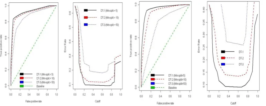
[image:5.595.78.515.331.505.2]Graphical results for both datasets are presented in Figure 1. Left to right, the first two panels correspond to Pima ROC and predictive patterns while the remaining two correspond to those of the Bupa dataset.
Figure 1. Pima (left) and Bupa(right) ROC curves and model over/fitting points
Based on the ROC convention, a classifier is optimal only if it yields results in the top left corner, given the set conditions. Thus, the performance ranking in both cases was DT-1, DT-2, and DT-3. The maximum differences (Youden Indices) between the TPR and FPR for each model, the areas under the curve, and the minimum prediction errors are highlighted in Table 3, agreeing with this ranking. Note that Bupa’s gaps between DT1 and DT2 and between DT2 and DT3 are much wider than Pima’s, implying that DT1 and DT2 performance on the Pima Indians data is almost indistinguishable. Further, repeated simulations are expected to vary depending on factors such as data sources and the settings defined in Section 2.2.
Table 3. Performance table for each of the three models on each of the two datasets
PIMA-1 PIMA-2 PIMA-3 BUPA-1 BUPA-2 BUPA-3
YOUDEN INDEX 0.7838 0.7392 0.5907 0.8128 0.7169 0.4583
AREA UNDER THE CURVE 0.9273 0.9086 0.8556 0.9527 0.9069 0.7487
[image:5.595.73.490.668.739.2]Accuracy of the test is a function of how well it separates the groups, and it is assessed by the corresponding area under the curve. Traditionally, a 90%-100% area under the curve is considered excellent while anything about 60% and less is a failure. Because ROC curves may mask or over-fit data estimated parameters, we propose a strategy for enhancing the formulation of a generalised error.
3.2 Proposed strategy for optimal model selection
Typically, one classifier is preferred to another if it yields a higher class posterior probability than the other (Web, 2005; Mwitondi, 2003). We have shown that the rate at which the models out-perform each other is data-dependent, and so the fitting patterns may provide a good starting point in the search for optimality. If we assume a Bayesian error from a notional population on which the performance of a predictive model is assessed to be (data-dependent error), then the relationship below holds.
( ) [ ] [ ] (8)
We can then measure model reliability by tracking the quantity [ ] as an indicator of stability/variability across models. The algorithm, described in the following simple steps, seeks to minimise the risk of over-fitting or under-fitting the data across applications.
Given a set of competing classifiers { } Extract the vectors and
Set For j:=1:K
For
Store the Differences DIFFS, TP and FP End For
Set a long bandwidth vector (typically Gaussian) ( ) While NOT END of Do
Compute and plot the densities of and End While
Examine the resulting plots and choose the one that best separates the groups End.
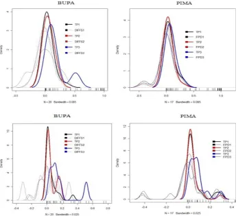
Figure 2. Differences between sequential TP and FP values and those of differences between them
The Gaussian kernel was used in approximating the differences in the algorithm. The optimal choice of the bandwidth is estimated as ( ̂⁄ ) ⁄ ̂ ⁄ (Silverman, 1984) where sigma is the standard deviation of the samples Runs based on these optimal bandwidth values yielded similar results to those in Figure 2 at suggesting DT1 for BUPA and DT2 for PIMA. Because each of the ROC curves in Figure 1 measures the probability that the corresponding model will rank a randomly chosen positive instance higher than it will rank a randomly chosen negative case, the patterns in Figure 2 provide an insight into the level of class separation and can be used to guide model selection.
4
CONCLUDING REMARKS AND POTENTIAL FUTURE DIRECTIONS
irrespective of the nature of the applications. We hope that this study will supplement previous studies that have focused on methods for selecting optimal models in our increasingly expanding cross-disciplinary research environment.
5
REFERENCES
Berger, J. O. (1985) Statistical Decision Theory and Bayesian Analysis, Springer-Verlag.
Breiman, L., Friedman, J. Stone, C. J., & Olshen, R. A. (1984) Classification and Regression Tree, Chapman
and Hall, ISBN-13: 978-0412048418.
Egan, J. P. (1975) Signal Detection Theory and Roc Analysis, Academic Press; ISBN-13 978-0122328503.
Freund, Y. & Schapire, R. (1997) A decision-theoretic generalization of on-line learning and an application to boosting. Journal of Computer and System Sciences 55 (1), pp 119–139.
Forsyth, R. S. (1990) PC/BEAGLE User's Guide, BUPA Medical Research Ltd.
Mwitondi, K. S. (2003) Robust Methods in Data Mining, PhD Thesis, School of Mathematics, University of
Leeds, Leeds, University Press.
Mwitondi, K. S. & Said, R. A. (2011) A step-wise method for labelling continuous data with a focus on striking a balance between predictive accuracy and model reliability. International Conference on the Challenges in Statistics and Operations Research (CSOR).
NIDDK (1990) Pima Indians Diabetes Data, National Institute of Diabetes and Digestive and Kidney Diseases.
Reilly, P. M. & Patino-Leal, H. (1981) A Bayesian Study of the Error-in-Variables Model. Technometrics 23,
(3).
Silverman, B. W. (1986) Density Estimation for Statistics and Data Analysis. Monographs on Statistics & Applied Probability, Chapman and Hall, ISBN-13: 978-0412246203.
Sing, T., Sander, O., Beerenwinkel, N., & Lengauer, T. (2005) ROCR: Visualizing Classifier Performance in R.
Bioinformatics 21 (20), pp. 3940-3941.
Youden, W.J. (1950) Index for rating diagnostic tests. Cancer 3, pp 32-35.