Overview: In this lab we will model a pendulum using frequency response (Bode plot) methods, plus

1

ECE-320 Lab 5: Modeling and Controlling a Pendulum

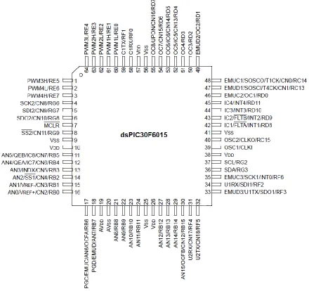
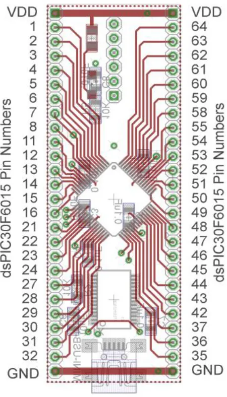
Overview: In this lab we will model a pendulum using frequency response (Bode plot) methods, plus some intuition about the form of the transfer function. We will be using the dsPIC30F6015 again, and this time we will be using a servo motor. For a servo motor we tell the motor where to go (what angular position) and it moves there on its own (it has an internal PID controller). We can also tell the motor how fast to move. Most of the initial code will be given to you (see the class website), and you will have to modify the code as you go on. The dsPIC30F6015 has been mounted on a carrier board that allows us to communicate with a terminal (your laptop) via a USB cable. In what follows you will need to make reference to the pin out of the dsPIC30F6015 (shown in Figure 1) and the corresponding pins on the carrier (shown in Figure 2)

3 Part A (Copying the initial files)

Set up a new folder for this lab, and copy the files for this lab from the class website to this folder.

Part B (Downloading and installing MPLAB) You will need to go to the website

https://www.microchip.com/pagehandler/en-us/family/mplabx/

and download the newest version of MPLABX. If you have an older of MPLAB it will probably work . It is probably easiest to download a zipped version and the unzip it. Do not intall any C compilers yet.

Part C (Downloading and installing MPLAB XC16 compiler) You will need to go to the website

https://www.microchip.com/pagehandler/en-us/family/mplabx/

and download the MPLAB XC16 compiler for the dsPIC. We want to use the free version of the compiler.

Part D (Setting up Communications with Secure CRT)

In this step we will make sure all of our systems are working before we go on.

Connect the PICkit3 to the carrier board and your computer (the white arrow goes near the white spot on the carrier board, or on the pin closest to the actual dsPIC chip.)

Connect the separate communication cable to the carrieer board and your computer.

Connect power to the power board and toggle to on switch (the green LED should then be on)

4 We are going to want to be able to record and plot data, so we will be writing to the screen. In order to do this we will using Secure CRT because it is installed on your computer by default.

Go to ProgramsAll ProgramsSecureCRTSecureCRT6.7 (it’s ok if you don’t have 6.7). You should get a screen like this (although the list of Sessions will probably be shorter for you):

5 You should then get a screen that looks like this

Click on New Session

Choose Serial from this menu, then click on Next at the bottom

6 You will next get the following screen. You should already know which port to use (it may not be

COM5 on your computer). Select a Baud rate of 115200 and be sure everything is filled in as below. The click on Next.

7 Finally, you may get a screen like that below, and if you do then you need to select Connect.

Now you should have a terminal like that shown below

8 Part E (Putting it all together)

Now we are ready to start. Note that at some point in the following process you may need to let the system download firmware. Be sure you have selected the correct device (or it will do this twice).

Start MPLAB X IDE (not IPE)

Select File, then New Project (the screen should default to Microchip Embedded and Standalone Project)

Click on Next

In the Select Device section, select the following:

Family: 16-bit DSCs (dsPIC30)

Device: dsPIC30F6015

Click on Next

In the Select Tool section, select PICkit3

Click on Next

In the Select Compiler section, select XC16

Click on Next

In the Select Project Name and Folder section, choose a name and project location.

Click on Finish

Make sure the file pendulum.cis in the Project folder. Right click on Source Files, then on Add Existing Item, then select pendulum.c.

9 For future reference, if you see the following message when trying to compile the program (don’t do this yet!)

You are trying to change protected boot and secure memory. In order to do this you must select the "Boot, Secure and General Segments" option on the debug tool Secure Segment properties page.

Failed to program device

Then

 Right Click on the Project Name (under Projects on the left panel) and select Properties  Under Categories in the left panel, click on PICkit3

 Under Option categories at the top, select Secure Segment  On the right select Boot, Secure, and General Segments  Then select ok at the bottom.

10 Part F (Implementing a stop button, this should already be done from previous labs)

Finally we need to set an external stop button for our system. This is particularly important once we connect a motor to the system since just stopping MPLABX does not shut off the motor by itself, and we need to be able to directly shut off the motor. There are two parts to our stop button- an LED that shows the system is armed (and disarmed) and a switch that is connected to an external interrupt (interrupt 4 in this case). Connect an LED and the switch as shown in the following figure:

Note that the interrupt is at a high voltage unless the switch is pushed. You should wire this so the switch is easily accessable.

11 Part G: Setting up the Second UART, the pendulum encoder, and the power.

In order to communicate with the servo motor, we will be using the second UART (UART2). To connect the motor control module to the dsPIC, connect the green wire to ground, the yellow wire to pin 32 (U2TX) , and the white wire to pin 31 (U2RX).

Next we need to connect the pendulum position encoder as shown in the figure below (the resistors are 10k )

Connect the servo motor to the motor control module using the white connector (there should be only one way to do this.) Note that there is a white connector on the motor part, and a white connector on the

motor control module. Do not confuse this with the pot connector connectect to the gear (which we are not using.)

Finally, connet the 12 volt power supply to the motor control module, this will power the servo motor.

Part H: Initial Communication

12 The light on the bottom of the motor control module should flash rapidly a few times and then flash slowly. The program should then write some information to to the screen. Most of this is making sure the parameters we are sending to the motor are being set correctly. For each of these parameters, we are writing to the motor and then reading back to see if the motor is set correctly. If any of them look incorrect (incorrect is most likely zero), push the interupt stop button, stop the program, and reload it and try again (including pushing down on the restart button.) The CW limit should be 100 degrees, and the CCW limit should be 200 degrees.

Once the program starts there are four items written to the SecureCRT screen. The first column should always be a 0. If it is a 1 then the program has not got to the end of the main while loop before the next interrupt has occurred, and the sampling rate is too high (note that writing to the screen is the primary cause of reduced speeds.) The second column is the time, the third column is the control signal (u) in radians, and the fourth column is the position of the pendulum (in radians.) The position of the

pendulum should initially be zero, and if you move the pendulum to the right (counter clock wise) you should get small negative numbers, and moving it to the left (clockwise) should produce small positive numbers. Do not go on until everythin in this part is working correctly.

Once this is done, you need to comment out the part of the code that disables the motor just before the main while loop (just before you set the control parameters.)

Part I: Determining the Frequency Response

In order to determine the magnitude portion of the frequency response, we need to input a cosine of a known amplitude and frequency, and record the output amplitude. We will not be measuring the phase portion of the frequency response in this lab.

In the code pendulum.c near the very end of the code in the main while loop, you need to uncomment and modify the following line of code:

u = 0.087*sin(TWO_PI*1.2*time);

Note that this line of code assume an input amplitude of 0.087 rad (5 degrees) and an input frequency of 1.2 Hz.

For the frequencies 1.2, 1.3, 1.4, 1.5 1.6, 1.7, 1.8, 1.9, 2.0, 2.25, 2.5 3.0 3.5, and 4.0 Hz, you need to do the following:

 Change the code for the desired frequency  Compile the code and download it.

 Start the code running

13  Look at the output written on the screen, particularly the last 10 seconds, and identify the

maximum positive output and the maximum negative output. Record the input frequency and the average of the absolute values of these amplitudes.

Open the Matlab program process_data_pendulum.m, and input the frequency, the input amplitude (0.087), and the average of the absolute values of the output amplitudes. Save this file, and then in the Matlab command window, type

data = process_data_pendulum

This will write to the array data, and write the frequency and gain at that frequency to the screen. Remember the frequency at which the maximum gain occurs.

Now we will fit this frequency response data to the transfer function

2 2 2 ( ) 2 p n n

G s Ks

s  s  

 

and we need to estimate the paramters K,  , and n.

To estimate these parameters we will use the Matlab program model_pendulum.m which utilizes Matlab’s fminsearch routine. The input arguments to model_pendulum.m are the array data, the initial guess of the parameter K (assume it is 1.0), the initial guess of the parameter  (assume it is 0.05), and the initial guess of the parameter _n (assume it is the frequency of the maximum gain, converted to

radians/sec.) The program spits a bunch of incredibly useful information to the screen, and eventually produces a plot of the transfer function and the measured data. The title indicates the estimated values of the parameters. If the transfer function does not seem to match the measured data very well you may want to try different initial estimates of the parameters, or rerun your system to check on the values you put into process_data_pendulum.m.

Assuming you do have reasonable estimates, you need to collect at least six additional data points, at least three near the peak and one on each side of the peak. Include your new data in

process_data_pendulum (you can add it to the end) and rerun all of the programs above. Include your final figure in your memo.

Part J: Comparing to the Step Response

14 In the program pendulum.c, uncomment the line position_pendulum() which is just inside the main while loop. This will set the pendulum to the middle of its range and then stop. Compile, download and run the program, then stop the program.

Now we want a step input, so comment out the lines

position_pendulum()

and

u = 0.087*sin(TWO_PI…)

Then uncomment the line

u = 10.0*PI/180.0;

Set up SecureCRT to log the recorded data to a file input_10_degree_step.

Compile, download, and run the program. You only need to run this for a few seconds. Then turn off the log function.

Edit the file plot_step_response_fit.m so the transfer function parameters fit your model, and make sure your are reading in the correct file. Run the program and be sure to include the figure in your memo. You should get a reasonable match between the model and measured systems. Note that this Matlab code converts your continuous-time transfer function to a discrete-time transfer function with a delay of two samples.

Part K: Designing and Implemmenting an I or a PI Controller

Our pendulum system is a regulator system, in that the goal is to hold the position of the pendulum in one place (downward at 0 degrees). This is somewhat different from a controller since the input value to the system is where we want the system to be. We want to look at how our regulator system responds to disturbances, which we will model as initial conditions.

Edit the Matlab file DT_PID_driver.m so the parameters of the transfer function match those you measured. Be sure the sample time Ts is also correct for your system (it should be 0.0175 seconds). You need to design an I or a PI controller (by guess and check) so the system returns to zero with as little “drama” as you can manage. In addition to changing the parameters of the controller you can also change the value of ISUM.

Once you feel you have a good regulator/controller you need to implement it in the program pendulum.c. This primarily involves commenting out any of the code that sets u to anything, and uncommenting the code

15 Before you try your regulator, you need to uncomment the code

postion_pendulum();

Compile, download, and run the system.(The pendulum should move to a center position.) Then comment this line of code out.

Before you go on, while the system is disconnected, tap the pendulum to get an idea of how fast it takes before the pendulum stops moving and returns to the zero position. However, try not to tap it so hard the base of the pendulum moves (its ok if it moves a little.)

Now that your regulator/controller is implemented, recompile, and download your code. Be sure you have also set ISUM to the value that you want. When you first start the system th pendulum may again move to the center position. Once the system is running, tap the pendulum and see how well it returns to the zero (down) position. It is ok if the base of the pendulum moves, since that is how we are trying to control the position of the pendulum. Again, the goal is to keep the pendulum pointed down compared to no regulator.

At this point you may want to try and improve on your regulator/controller, so you need to iterate a bit. It is likely to “twitch” a bit (twitch being a technical term) since we are dealing with errors in

measurement and limted control over the motor. Do the best you can here. When you feel you have a good system log the data for about 20 seconds and tap the pendulum. Plot the motion of the pendulum in Matlab and include this figure in your memo.

Part L: Refining Your Controller

There is one last thing we can play with in our system to try and change the response of the motor. Right now the motor is set to move as fast as possible which sometimes actually induces motion in the

pendulum.

In the code pendulum.c, in the routine setup_motor, the line of code

bob = sprintf(sbuf,”%c1023\r”,send);

controls the speed of the motor. We can approximately model our motor speed using the equation 0.01168* 0.017

motor speed B

Where speed is the motor speed in radians/sec and B is an integer between 1 and 1023. Note that you need to include four digits in the code for the motor speed. For example, if you want the motor speed to be 64, you need to use the code