ECE-420: Discrete-Time Control Systems Homework 3
Due: Thursday September 25 at 5 PM Exam 1, Friday September 26
1) Consider the continuous-time plant with transfer function 1 ( )
( 1)( 2) p s s G s
We want to determine the discrete-time equivalent to this plant, Gp( )z , by assuming a zero order hold is placed before the continuous-time plant to convert the discrete-time control signal to a continuous time control signal.
Show that if we assume a sampling interval of T, the equivalent discrete-time plant is
2 2 3
2
(0.5 0.5e ) (0.5 0.5 )
( )
( )( )
T T T T T
p T T
z e e e e
G z
z e z e
Note that we have poles were we expect them to be, but we have introduced a zero in going from the continuous time system to the discrete-time system.
2) In this problem assume the feedback configuration shown below.
a) Assume
1 0 1
0 , ( ) , ( ) ( ) 1 c c p p c
b z b
G z G z
H z z b
z
If the plant is equal to 3 and we want all of the closed loop poles at -0.5, show that the controller and closed loop transfer functions are
2 2 1 (2 0.25) 3 12 ( ) , ( ) 1 0.25 c o z z z z z
G z G z
z
b) Assume
0 1 0
( ) b , ( )
) 1,
1 (
c c p
c p P
b z b
z G z
H z
z z a
G
If the plant is equal to 2 0.5
z and the closed loop poles are at -0.5 and -0.333, show that the controller
and the closed loop transfer function are
2
1.167 0.167 2.333 0.333
( ) , ( )
1 0.833 0.167
c o
z z
G z G z
z z z
3) The file zoh_files.slxand zoh_driver.m illustrate how to model discrete-times systems from continuous-time systems in both Matlab and Simulink.
The first system in zoh_files.slx illustrates how to utilize a sample and hold and a zero order hold to allow modelling a continuous-time system as a discrete-time system.
The second system is the equivalent discrete-time constructed in Matlab. If you run the file zoh_driver.m you should see the results of the two simulations lie on top of each other.
The third system is a continuous-time state variable model of an open loop plant.
The fourth system is the equivalent discrete-time state variable system with state variable feedback modelled in Matlab.
For this problem, you need to modify the third system using sample and hold(s) and zero order hold(s) so you can model the system as a discrete-time system and include state variable feedback. For this problem turn in your plot of the outputs (the Matlab and Simulink should be the same) and print your zoh_files.slx file (so I can see it). This problem should be very simple, but I want you to have to see how to do some of these things in Matlab and Simulink.
Note that we can write the discrete-time state equations as
( 1) ( ) ( )
( ) ( ) ( )
x n Gx n Hu n y n Cx n Du n
4) (sisotool) The file DT_PID.mdl is a Simulink model that implements a discrete-time PID controller. It is somewhat unusual in that the plant is represented in state-variable form, but this is the usual form we will be using in this class. The Simulink model looks like the following:
The file DT_PID_driver.m is the Matlab file that runs this code. We will be utilizing Matlab’s sisotool
for determining the pole placement and the values of the gains.
Before we go on, we need to remember the following two things about discrete-time systems:
For stability, all poles of the system must be within the unit circle. However, zeros can be outside of the unit circle.
The closer to the origin your dominant poles are, the faster your system will respond. However, the control effort will generally be larger.
The basic transfer function form of the components of a discrete-time PID controller are as follows:
Proportional (P) term : C z( )K E zp ( ) Integral (I) term: ( ) 1
1 1
i i
K K z
C z
z z
Derivative (D) term : ( ) (1 1) d( 1) d
K z
C z K z
z
PI Controller: To construct a PI controller, we add the P and I controllers together to get the overall transfer function:
( )
( )
1 1
p i p
i p
K K z K K z
C z K
z z
In sisotool this will be represented as
2
( ) ( )
( )
( 1) ( 1)
K z az K z a
C z
z z z
In order to get the coefficients we need out of the sisotool format we equate coefficients to get:
PID Controller: To construct a PID controller, we add the P, I, and D controllers together to get the overall transfer function:
2 2 2
( 1) ( 1) ( ) ( 2 )
( 1)
( )
1 ( 1) ( 1)
p i d p i d p d d
i d
p
K z z K z K z K K K z K K z K
K z K z
C z K
z z z z z z
In sisotool this will be represented as
2
( )
( )
( 1)
K z az b
C z
z z
In order to get the coefficients we need out of the sisotool format we equate coefficients to get:
, 2 ,
d p d i p d
K Kb K Ka K K K K K
For the PID controller, we can have either two complex conjugate zeros or two real zeros.
Note that these calculations are pretty much done for you in the driver file DT_PID_driver.m
The file DT_PID_driver implements a controller for the default plant 3 9.348 2 8.
0.88 879 ( )
1.495 49
p
z z
z z z
G
assuming a sampling interval of Ts 0.1 seconds.
You may want to read the review of sisotool at the end of this homework before going on.
For the remainder of this problem, you are to design two controllers for the plant
3 2
12
( ) 5
1.9 0.5 p G z z z z z
assuming a sampling interval of 0.1 seconds.
A) Modify the default plant in the Matlab program DT_PID_driver.m and run the program. This
program is set up to implement a P controller for the default plant with gain 0.0116. It will put the value of the transfer function for the system, G zp( ), in your workspace.
B) Start sisotool and load in the transfer function. It is easiest to get the parameters you need if you use the pole-zero form of the controller. To do this type
Edit → SISO Tool Preferences → Options and click on zero/pole/gain.
D) Use sisotool to determine a PID controller (I would suggest real zeros, but it is up to you!) so the system has a settling time less than 2.5 seconds and a percent overshoot less than 15%. The control effort must also be within the allowed bounds. Print out the root locus plots and the step response using DT_PID_driver.m and print out the graph. Include the values of k kp, ,i and k with your d graph.
Sisotool (Brief) Example
Run the Matlab program DT_PID_driver.m. This program is set up to implement a P controller with gain 0.0116. It will put the value of the transfer function for your system,G zp( ), in your workspace.
Now we are ready for sisotool.
Getting Started
Type sisotool in the command window
Click close when the help window comes up
Click on View, then Design Plots Configuration, and turn off all plots except the Root Locus plot (set the Plot Type to Root Locus for Plot 1, and set the Plot Type to None for all other Plots)
Loading the Transfer Function
In the SISO Design window, Click on file → import.
We will usually be assigning Gp(z) to block G (the plant). Under the System heading, click on the line that indicates G, then click on Browse.
Choose the available Model that you want assigned to G (Click on the appropriate line) and then click on Import, and then on Close.
Click OK on the System Data (Import Model) window
Once the transfer function has been entered, the root locus is displayed. Make sure the poles and zeros of your plant are where you think they should be.
Generating the Step Response
Click on Analysis → Response to Step Command (the system is unstable at this point)
You will probably have two curves on your step response plot. To just get the output, type Analysis → Other Loop Responses. If you only want the output, then only r to y is checked, and then click OK. However, sometimes you will also want the r to u output, since it shows the control effort for P, I, and PI controllers.
You can move the location of the pole in the root locus plot by putting the cursor over the pink button and holding the left mouse button down as you move the pole locations. You should note that the step response changes as the pole locations change.
Entering a Compensator (controller): We will implement a PI controller here
Click on Designs, then Edit Compensators.
Right click in the Dynamics window to enter real poles and zeros. You will be able to changes these values very easily later. Since we want a PI controller, we need a pole to be a 1 and we need to be able to change the value of the zero. For now assume the zero is at -1.
Look at the form of C to be sure it's what you intended, and then look at the root locus with the compensator.
You can again see how the step response changes with the compensator by moving the locations of the zero (grab the pink dot and slide it) and moving the gain of the system (grab the squares and drag them). Remember we need all poles and zeros to be inside the unit circle for stability!
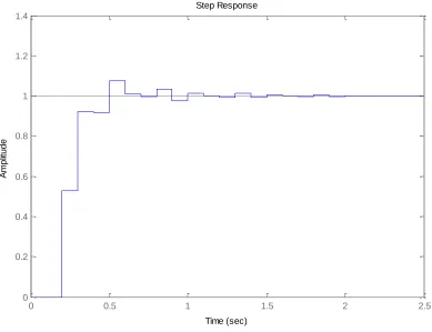
[image:7.612.119.508.283.582.2] Move the pole and zero around until the zero is approximately -0.295 and the gain is approximately 0.0563. You should get a figure like that shown in Figure 1.
Figure 1. Discrete-time example with w PI controller.
Adding Constraints
Right Click on the Root Locus plot, and choose Design Requirements then either New to add new constraints, or Edit to edit existing constraints.
At this point you have a choice of various types of constraints.
Remember these constraints are only exact for ideal second order systems!!!!!
Step Response
Time (sec)
A
m
p
lit
u
d
e
0 0.5 1 1.5 2 2.5
Printing/Saving the Figures:
To save a figure sisotool has created, click File → Print to Figure
Odds and Ends :
You may want to fix the axes. To do this,
Right click on the Root Locus Plot
Choose Properties
Choose Limits
Set the limits and turn the Auto Scale off
You may also want to put on a grid, as another method of checking your answers. To do this, right click on the Root Locus plot, then choose Grid