ECE 300 Signals and Systems Fall 2005 RDT
Measurement of Fourier Coefficients
Lab 05
by Bruce A. Black with some tweaking by others
Objectives
• To measure the Fourier coefficients of several waveforms and compare the measured values
with theoretical values.
• To become acquainted with the Agilent E4402B Spectrum Analyzer.
Equipment
Agilent E4402B Spectrum Analyzer Agilent Function Generator
Oscilloscope BNC T-Connector
Background
Recently we learned to calculate the line spectrum of a periodic signal by using the Fourier
series. We have in our lab spectrum analyzers that can display the spectrum of a signal in
pseudo- real time. The Agilent E4402B Spectrum Analyzer (SA) can be used to view the power
spectrum of any signal of frequency up to 3 GHz. The SA displays a “one-sided spectrum” in decibels (dBs) versus frequency. In lab we will observe the spectra of sinusoids, square and triangle waves, and pulse trains, but first we must learn how to convert the Fourier series coefficients that we calculate to the dB values displayed by the spectrum analyzer.
Recall that any periodic signal x t
( )
can be written as( )
2 00 0
, where 1
j kf t k k
x t a e π f
∞
=−∞
=
∑
= T .Writing out a few terms gives
( )
0 0 0 00 0 0
2 1 1 2
2 2 2 2 2 2
2 1 0 1 2
2 2 2 2 2 2
2 1 0 1 2
j f t j f t j f t j f t
j f t j f t j f t j f t
j a j a j a j a
x t a e a e a a e a e
a e e a e e a a e e a e e
π π π π
π π π π
− −
− −
− −
− −
= + + + + + +
= + + + + + 0 +
k
(1)
where we have used the fact that a−k =a∗ whenever x t
( )
is real-valued. Notice that, aside from, the terms come in pairs (actually, complex conjugate pairs). We can combine each positive-frequency term with its matching negative positive-frequency term to obtain
0
a
( )
0 2 1 cos 2(
0 1)
2 2 cos 2 2(
0 2)
x t =a + a πf t+ a + a π f t+ a + . (2)
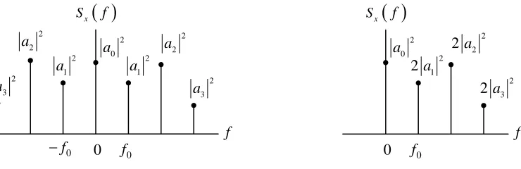
to be ak 2 (and corresponds most directly with equation (1)). The corresponding one-sided power spectrum is shown in Fig. 2. To make the one-sided spectrum, the powers associated with
complex exponentials at frequencies kf0 and −kf0 are added. The result, representing the
average power in the sinusoid 2 ak cos 2
(
πf tk + ak)
, is shown at frequency (andcorresponds most directly with equation
[image:2.612.106.476.178.298.2]0 kf (2)).
( )
x S f f 0 f 0 f − 2 0 a 2 1 a 2 1 a 2 2 a 2 2 a 2 3 a 2 3 a 0( )
x S f f 0 f 2 0 a 2 1 2a 2 2 2a 2 3 2 a 0Figure 1: Two-Sided Power Spectrum Figure 2: One-Sided Power Spectrum
The SA displays a one-sided spectrum as shown in Fig. 2, but instead of showing the value of
2
2ak at each frequency, the spectrum analyzer shows average power in decibels with respect to
a one millivolt RMS reference. For the sinusoid at frequency , the average power in decibels
is given by
0
kf
10
10 log k
k dB ref P P P = ,
where the power Pk represents the power spectrum coefficient
2
2ak , and the power Pref is the
average power delivered to a one-ohm resistor by a one millivolt RMS sinusoid. We have
(
)
2
2
2
10 log dBmV
0.001 k k dBmV
a
P = .
The units “dBmV” indicate that the reference for the decibels is a one millivolt RMS sinusoid.*
[image:2.612.93.274.179.298.2]Pre-Lab
1. Calculate the Fourier series coefficientsak, k= ± ±0, 1, 2,…, 9± , for each of the three waveforms given below. Be sure your results make sense. It is recommended that you produce a plot of the waveform produced by your Fourier Series coefficients to verify their accuracy.
2. Calculate the decibel power level (dBmV) that you expect will be displayed by the spectrum
analyzer for each term, again for each waveform.
3. For each waveform, create a table in your lab notebook containing a column of values of
and a column of values of predicted decibel levels. Leave two additional blank columns, one for measured decibels and one for dB difference. (Note that % difference is
k a
not the correct error measure when measuring in dBs.)
4. Read the documents “SA_hints_E4402B” and “Reading_SA_Display_E4402B”, both
available on the spectrum analyzer webpage.
The waveforms, each having zero DC offset, are:
a) x t1
( )
=0.1cos 2 100 10(
π × 3t)
Vb) x2
( )
t is a square wave of period 10 μs and peak-to-peak amplitude 0.2 V.c) x t3
( )
is a triangle wave of period 10 μs and peak-to-peak amplitude 0.2 V.Just to be sure there is no confusion regarding the waveforms, they are displayed below.
a) b)
Procedure
Getting Ready
Before connecting any input to the spectrum analyzer, be sure that there is no large DC offset on the signal – in our case, no DC offset should be contained in the signal. The only sure way to know this is to properly examine the signal on the oscilloscope. Be sure you understand the implications of the different input impedance of the scope and the spectrum analyzer before you begin this lab.**
Measuring the Spectrum
1. Use the function generator to generate a sinusoid of frequency 100 kHz and (open circuit)
amplitude 0.1 V (waveform a). Use the oscilloscope to verify the amplitude**. Now observe the signal power spectrum on the spectrum analyzer. Measure the power level and frequency. Compare with your pre-lab calculations. Provide a plot the SA display, indicating important features, in your notebook.
Informally vary the frequency and the amplitude of the sinusoid and observe how the spectrum analyzer display changes. Record your observations
2. Use the function generator to generate a square wave of period 10 μs and peak-to-peak
amplitude 0.2 V (waveform b). Using the spectrum analyzer, measure the level of the first nine harmonics. Compare with the values you calculated in the pre-lab. Provide a plot the SA display, indicating important features, in your notebook.
3. Use the function generator to generate a triangle wave of period 10 μs and peak-to-peak
amplitude 0.2 V (waveform c). Use the spectrum analyzer to measure the level of the first nine harmonics. Compare with the values you calculated in the pre-lab. Provide a plot the SA display, indicating important features, in your notebook.
4. Now use the function generator to generate a pulse train having a period of 10 μs, a
peak-to-peak amplitude of 0.2 V and a duty cycle of 20%. (The “duty cycle” is the pulse width divided by the period.) Measure the spectrum using the spectrum analyzer. Provide a plot the SA display, indicating important features, in your notebook. Identify the flowing features of the spectrum: envelope of the spectrum (overall shape), the frequency of the nulls of the envelope, and the frequency locations of the various spectral components. You may need to observe a wider range of frequencies to see these features. Compare the spectrum with the spectrum of the “plain” square wave.
5. Take data that will allow you to quantitatively answer the following questions:
(c) What happens when the duty cycle is fixed, but the pulse period is changed? Be sure to record and explain the changes to all the spectral features.
Report
In your lab notebook present your theoretical results, measured results, comparisons, comments, and answers to the questions posed above. Be sure that all members of your lab group sign the lab notebook, and hand the notebook in at the end of lab.
** Note concerning Agilent FG amplitude readings
The Agilent function generators have an interesting feature built into their displays. The FG is a
50 Ω output impedance device, designed to deliver maximum power to a 50 Ω load. The FG by
default will display the voltage amplitude delivered to a 50 Ω load, independent of what is
actually connected. By changing the display setting to “High-Z”, the FG display will display the voltage delivered to a high impedance load, assuming a high impedance load is connected.
However, the FG remains a 50 Ω output impedance device. Since the scope and spectrum