2) Using the Digilent EE bread board construct the circuit shown in Figure 1 using your 1 f capacitor and a 1

1

ECE-205 Lab 2

Introduction to the Digilent EE Board

Throughout this lab we will focus on the use of the Digilent Electronics Explorer board for measuring the response of first and second order circuits. Our goal is to become familiar with some of the features of this board and how to use it.

The end result of this Lab will be a memo written to me that includes the figures you generated. Each figure needs to have a figure number and a caption. The body of the memo should be fairly short (less than one paragraph). Do not reiterate what you did in the lab, but tell me what parts of the lab were confusing, what you liked and what you didn’t like.

Part A

1) Obtain a 1 µf capacitor and a 1 kΩ resistor from you lab kit. Using an R/L/C meter measure the actual values for the resistor and the capacitor and record them in your memo. Your estimated time constant for your circuit should be τ =RC and you should use this value in the result of the lab. This value should be near 1 ms, but it may be up to 20% off.

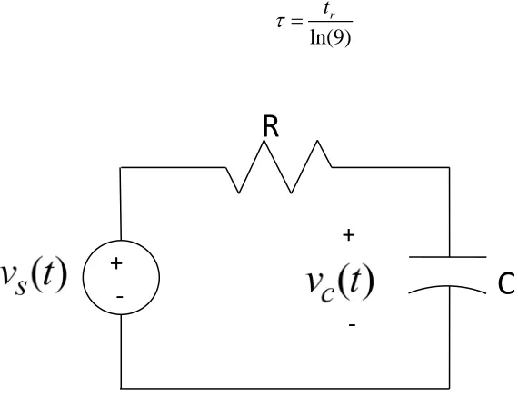
2) Using the Digilent EE bread board construct the circuit shown in Figure 1 using your 1 µf capacitor and a 1 kΩ resistor. These components should be available in your lab kit. We will measure the output of the circuit as the voltage across the capacitor. We will be trying to estimate the time constants for this circuit as we vary the resistance. The time constant for this circuit is τ =RC, and we will measure the time constant by determining the 10%-90% rise time, t_r, and using the formula

ln(9)

r

t

τ =

Figure 1. Circuit for Part A.

2 2) As you build this circuit, there are a few things you should do and notice

• In this class we will be using the Analog side of the board. The right hand side of the Scope, Analog, and Power components are grounded. Use a short wire to jumper one of these grounds to the blue rail, so we have a common ground for all of your circuits.

• The voltage source is AGW1 (use the left pin) from the Analog block. The ground is common so you do not need to connect a ground. Just use a wire from AGW1 to the resistor.

• The EE board measures voltages with respect to ground. Since we want to measure the voltage across the capacitor, and one pin of the capacitor is connected to ground, we just need to connect a wire from the Scope block, to the positive side of the capacitor. Let’s connect a wire from terminal DC1 to the positive end of the capacitor. For the scope, DC means we are using DC coupling, while AC means we are using AC coupling. If we use DC coupling we can have a nonzero average signal, which is what we want now.

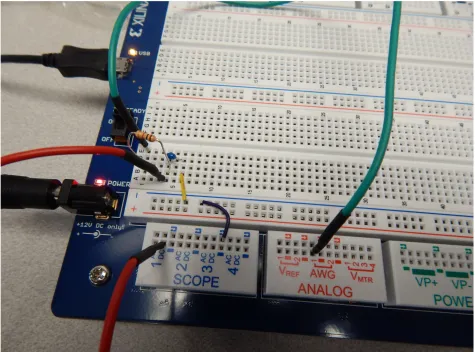
My final wiring for this circuit looked like that shown in Figure 2.

3 3) Start Digilent Waveforms.

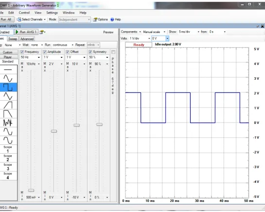
4) Start the Function Generator. Set channel 1 to a 50 Hz square wave, with a 1 DC offset and peak to peak value of 2.0 volts (the amplitude of the waveform will be 1 Volt). The symmetry should be set to 50%. If your range of frequencies or volts is not in the menu, select the upper or lower value that you want to change, Set channel 2 to a zero output (we will not be using it). The scope channel should look something like that shown in Figure 3 once you have started the waveform generator. (Note that I have used the Settings-> Options to set my waveform to blue.)

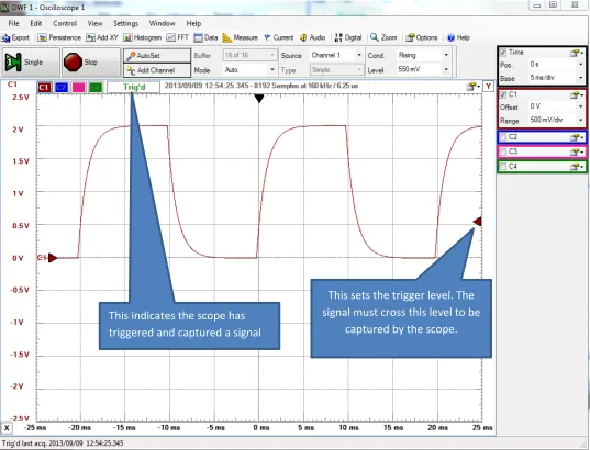
4 5) Start the Oscilloscope. Turn off all of the channels except C1. Set the Time Base to 5 ms/div and for C1 set the scale to 500 mV/div with and offset of 0 volts. If you select the pull down menu at the right of the C1 channel box, you can change some of the parameters. I have changed the color for the signal on mine. If you start the scope and the waveform generator is on, your oscilloscope channel should look more or less like that in Figure 4. However, it may not and that will be explained shortly.

There are two important things to check on this figure, or whenever you use a scope. The first is to make sure you have “triggered”. The scope captures a signal once the signal has crossed the trigger level or threshold. If you do not see any signal and the scope has not triggered, change the trigger level by moving the trigger level (see Figure 4.)

Note that if you “right click” in the scope screen, there are many options to choose.

Figure 4. Oscilloscope screen for channel 1 for Part A. This indicates the scope has

triggered and captured a signal

This sets the trigger level. The signal must cross this level to be

5 6) Next we want to make measurements on our signal. In the scope window, right click the mouse and select HotTrack. This may have the effect of suddenly filling your screen with way more information than you wanted. We will first use these cursors to measure the rise time, and hence the time constant of our circuit.

7) If your Digilent EE board is reasonably calibrated, your output signal should go from approximately zero volts to 2 volts. We need to measure the rise time (t_r ) or the time it takes the signal to go from 10% to 90% of its final value. Using the cursors, determine the time your signal takes to go from 0 to 0.2 volts (10% of 2.0 volts), and from 0 to 1.8 volts (90% of 2.0 volts). The difference in time is the rise time (subtract the 0 to 10% time from the 0 to 90% time). Using this rise time, compute the time constant using the formula

ln(9)

r

t

τ =

Your time constant should be very close to the time constant you computed in step 1 for this circuit. Compute your percent error, and if it is more than 20% off ask for help. Record your work computing your error and include it in your memo.

8) We can actually use the built in functions to determine the rise time (which is the same as the fall time, by the way). At the top of the scope screen, select Measure (there is a yellow triangle next to it). Then select + Add, then Channel 1, then Horizontal, then Rise Time then Average. Click on the green + Add selected

measurement to add this measurement to the measurement window. Compute the time constant again with this value of the rise time.

9) Add the Fall Time to the measurements, and use this to estimate the time constant.

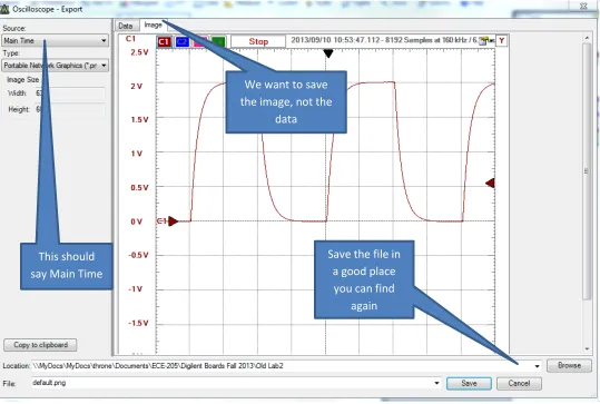
10) Next we want to capture a screen shot to put into your memo. Near the top left corner of the oscilloscope is the Export icon. Click on this icon, and you will get a figure somewhat like that shown in Figure 5 (See next page.) On the left you want to select Main Time and above the image you want to select Image instead of Data. Save this screen shot to a file. Then (right now!) include this screen shot in your memo for this lab. Do not wait to see if it all worked out! Put in a figure number and an appropriate caption.

Part B

We are now going to repeat the above procedures for two different time constants. Hopefully you will get more of a feel for what a time constant means by doing this. In what follows, be sure your signal has reached steady state. This means it is not changing and is basically flat. It should start and end flat (the slope of the signal is zero)

1) Replace the 1 kΩ resistor with the variable resistor in your lab kit. One of the outside pins should not be connected to anything. That is, to use this as a variable resistor the input is one of the outside pins and the output is the middle pin (or you could do it the other way).

2) Adjust the variable resistor so the rise/fall time is between 0.5 and 0.6 ms. Capture a screen shot of the waveform and the measurement to include in your memo. This time choose Main Window as the source so it will show the measurements. Put this figure in your memo with a figure number and an appropriate caption.

6

or it is wrong and you will have to do this again! Capture a screen shot of the waveform and the measurement

to include in your memo. This time choose Main Window as the source so it will show the measurements. Put this figure in your memo with a figure number and an appropriate caption.

Figure 5. Saving a screen shot.

Part C

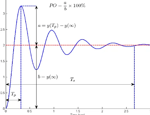
In this part, we will look at the response of a second order circuit and how changing the damping ratio changes the characteristic of the output. The Figure 6 shows some of the important characteristics we usually measure for the step response for an underdamped second order systems. These include the Percent Overshoot (PO), the steady state value (y(∞)), the Time to Peak (T_p), and the Settling Time (T_s). In this part of the lab we are mostly interested in the percent overshoot.

This should say Main Time

We want to save the image, not the

data

Save the file in a good place

7 Figure 6. Important characteristics of the step response of an underdamped second order system.

1) Construct the second order circuit shown in Figure 7. For this circuit, use your variable resistor for R, use a 0.01 µfcapacitor, and a 33 mH inductor.

Figure 7. Second order circuit for Part C

+ -

8 2) Set up the Digilent EE board to provide the input and measure the output. The input should be a square wave with frequency between 500 Hz and 1.5 kHz with a 0.5 volt offset and 1 volt peak to peak. You should change the time access on the Arbitrary Waveform Generator screen so you get a good signal with only a few periods. This will help you decide how to set the time scale on the scope.

3) Set the variable resistor somewhere in the middle of its range just so we can get an output signal. The output is the voltage across the capacitor. Since all measurements are with respect to ground, and we want to measure the voltage across the capacitor, you will need to use two channels on the scope. Connect DC Channel 1 to the positive side of the capacitor, and connect DC Channel 2 to the negative side of the capacitor. Once you have connected these wires and see some signals on the scope, turn off channels 1 and 2. Now right click on the mouse somewhere in the space below the channel selectors and select Add Mathematical Channel -> Simple. This allows us to make simple calculations using the channels we have. We want the output to be C1 minus C2, so modify channel M1 so this is true. (You should also change the scaling to get a good picture on the scope.)

4) The parameters for this problem are _n 1

LC

ω = and

2

R C L

ζ = , so by varying the resistor we can directly

vary the damping ratio but not change the natural frequency.

5) Choose a resistance to provide no overshoot. Try to get as close to no overshoot as you can though. Export the scope shot of your waveform, and put it in your memo. Be sure to number your figure, and give it a good caption.

6) Choose a resistance to provide an overshoot between 40 and 50%. Use the cursors to verify the overshoot. (Do not use the measurement function for this, it does not measure percent overshoot the same way we do.) Export a scope shot of your waveform and put it in your memo. Be sure to number your figure, and give it a good caption. Include your calculation of the overshoot in your memo.

Part D

Now we want to measure the time constant for an unknown first order system. This is what you will be doing for part of your Lab Practical, so pay attention!! Get a numbered black box from your instructor and write the number down. Place the circuit so you can read the numbers. The red connectors are the positive terminals and should be on top, and the black connectors are the ground terminals and should be on the bottom. The

instructions below are a bit vague, since you should have an idea of how to do this and each system is different.

1) Using the alligator clips, connect the signal generator AWG1 to the left side of the box, and the scope to the right side. Connect one of the two ground wires to the Digilent EE ground..

2) Set the input signal to a square wave with an offset of 0.5 volts and 0.5 volt amplitude (1 volt peak to peak, with the lowest value 0 and the highest value 1.0)

3) Set the time scales so you get a reasonable plot on the scope, and you get enough periods that there is a good estimate of the rise or fall times (no ? in the estimate boxes)

4) Determine the time constant and check with your instructor to determine if your value is acceptable

9