Combining Relational and Distributional Knowledge for Word Sense Disambiguation

Combining Relational and Distributional Knowledge

for Word Sense Disambiguation

Richard Johansson Luis Nieto Pi ˜na

Spr˚akbanken, Department of Swedish, University of Gothenburg Box 200, SE-40530 Gothenburg, Sweden

{richard.johansson, luis.nieto.pina}@svenska.gu.se

Abstract

We present a new approach to word sense disambiguation derived from recent ideas in distributional semantics. The input to the algorithm is a large unlabeled cor-pus and a graph describing how senses are related; no sense-annotated corpus is needed. The fundamental idea is to em-bed meaning representations of sensesin the same continuous-valued vector space as the representations of words. In this way, the knowledge encoded in the lex-ical resource is combined with the infor-mation derived by the distributional meth-ods. Once this step has been carried out, the sense representations can be plugged back into e.g. the skip-gram model, which allows us to compute scores for the differ-ent possible senses of a word in a given context.

We evaluated the new word sense dis-ambiguation system on two Swedish test sets annotated with senses defined by the SALDO lexical resource. In both evalu-ations, our system soundly outperformed random and first-sense baselines. Its ac-curacy was slightly above that of a well-known graph-based system, while being computationally much more efficient. 1 Introduction

For NLP applications such as word sense disam-biguation (WSD), it is crucial to use some sort of representation of the meaning of a word. There are two broad approaches commonly used in NLP to represent word meaning: representations based on the structure of a formal knowledge representa-tion, and those derived from co-occurrence statis-tics in corpora (distributionalrepresentations). In a knowledge-based word meaning representation,

the meaning of a word string is defined by map-ping it to a symbolic concept defined in a knowl-edge base or ontology, and the meaning of the con-cept itself is defined in terms of its relations to other concepts, which can be used to deduce facts that were not stated explicitly: amouseis a type ofrodent, so it has prominentteeth. On the other hand, in a data-driven meaning representation, the meaning of a word in defined as a point in a ge-ometric space, which is derived from the word’s cooccurrence patterns so that words with a similar meaning end up near each other in the vector space (Turney and Pantel, 2010). The most important re-lation between the meaning representations of two words is typicallysimilarity: amouseis something quite similar to arat. Similarity of meaning is of-ten operationalized in terms of the geometry of the vector space, e.g. by defining a distance metric.

may correspond to more than one underlying con-cept. For instance, the word mouse can refer to a rodent or anelectronic device. Except for sce-narios where a small number of senses are used, lexical-semantic resources such as WordNet (Fell-baum, 1998) for English and SALDO (Borin et al., 2013) for Swedish are crucial in applications that rely on sense meaning, WSD above all.

Corpus-derived representations on the other hand typically have only one representation per surface form, which makes it hard to search e.g. for a group of words similar to the ro-dent sense of mouse1 or to reliably use the vec-tor in machine learning methods that generalize from the semantics of the word (Erk and Pad´o, 2010). One straightforward solution could be to build a vector-space semantic representation from a sense-annotated corpus, but this is infeasible since fairly large corpora are needed to induce data-driven representations of a high quality, while sense-annotated corpora are small and scarce. In-stead, there have been several attempts to cre-ate vectors representing the senses of ambiguous words, most of them based on some variant of the idea first proposed by Sch¨utze (1998): that senses can be seen as clusters of similar contexts. Fur-ther examples where this idea has reappeared in-clude the work by Purandare and Pedersen (2004), as well as a number of recent papers (Huang et al., 2012; Moen et al., 2013; Neelakantan et al., 2014; K˚ageb¨ack et al., 2015). However, sense dis-tributions are often highly imbalanced, it is not clear that context clusters can be reliably created for senses that occur rarely.

In this work, we build a word sense disambigua-tion system by combining the two approaches to representing meaning. The crucial stepping stone is the recently developed algorithm by Johansson and Nieto Pi˜na (2015), which derives vector-space representations of word senses by embedding the graph structure of a semantic network in the word vector space. A scoring function for selecting a sense can then be derived from a word-based dis-tributional model in a very intuitive way simply by reusing the scoring function used to construct the original word-based vector space. This approach to WSD is attractive because it can leverage corpus statistics similar to a supervised method trained on an annotated corpus, but also use the

lexical-1_{According to Gyllensten and Sahlgren (2015), this}

prob-lem can be remedied by making better use of the topology of the neighborhood around the search term.

semantic resource for generalization. Moreover, the sense representation algorithm also estimates how common the different senses are; finding the predominant sense of a word also gives a strong baseline for WSD (McCarthy et al., 2007), and is of course also interesting from a lexicographical perspective.

We applied the algorithm to derive vector rep-resentations for the senses in SALDO, a Swedish semantic network (Borin et al., 2013), and we used these vectors to build a disambiguation system that can assign a SALDO sense to ambiguous words occurring in free text. To evaluate the system, we created two new benchmark sets by processing publicly available datasets. On these benchmarks, our system outperforms a random baseline by a wide margin, but also a first-sense baseline signif-icantly. It achieves a slightly higher score than UKB, a highly accurate graph-based WSD sys-tem (Agirre and Soroa, 2009), but is several orders of magnitude faster. The highest disambiguation accuracy was achieved by combining the proba-bilities output by the two systems. Furthermore, in a qualitative inspection of the most ambiguous words in SALDO for each word class, we see that the sense distribution estimates provided by the sense embedding algorithm are good for nouns, adjectives, and adverbs, although less so for verbs. 2 Representing the meaning of words

and senses

In NLP, the idea of representing word meaning geometrically is most closely associated with the distributional approach: the meaning of a word is reflected in the set of contexts in which it ap-pears. This idea has a long tradition in linguistics and early NLP (Harris, 1954).

Dumais, 1997; Kanerva et al., 2000).

As an alternative to context-counting vectors, geometric word representations can be derived in-directly, as a by-product when training classifiers that predict the context of a focus word. While these representations have often been built using fairly complex machine learning methods (Col-lobert and Weston, 2008; Turian et al., 2010), such representations can also be created using much simpler and computationally more efficient log-linear methods that seem to perform equally well (Mnih and Kavukcuoglu, 2013; Mikolov et al., 2013a). In this work, we use theskip-grammodel by Mikolov et al. (2013a): given a focus word, the contextual classifier predicts the words around it. 2.1 From word meaning to sense meaning The crucial stepping stone to WSD used in this work is toembedthe semantic network in a vec-tor space: that is, to associate each sensesi jwith a

sense embedding, a vectorE(si j)of real numbers, in a way that makes sense given the topology of the semantic network but also reflects that the vectors representing the lemmas are related to those corre-sponding to the underlying senses (Johansson and Nieto Pi˜na, 2015).

Figure 1 shows an example involving an ambiguous word. The figure shows a two-dimensional projection2 of the vector-space rep-resentation of the Swedish wordrock(meaning ei-ther ‘coat’ or ‘rock music’) and some words re-lated to it: morgonrock ‘dressing gown’, jacka ‘jacket’, kappa ‘coat’, oljerock ‘oilskin coat’, l˚angrock ‘long coat’, musik ‘music’, jazz ‘jazz’, h˚ardrock ‘hard rock’,punkrock‘punk rock’,funk ‘funk’. The words for styles of popular music and the words for pieces of clothing are clearly sepa-rated, and the polysemous wordrock seems to be dominated by its music sense.

The sense embedding algorithm will then pro-duce vector-space representations of the two senses ofrock. Our lexicon tells us that there are two senses, one related to clothing and the other to music. The embedding of the first sense (‘coat’) ends up near the other items of clothing, and the second sense (‘rock music’) near other styles of music. Furthermore, the embedding of the lemma consists of a mix of the embeddings of the two

2_{The figures were computed in scikit-learn}

(Pe-dregosa et al., 2011) using multidimensional scaling of the distances in a 512-dimensional vector space.

senses: mainly of the music sense, which reflects the fact that this sense is most frequent in corpora.

rock

rock-1 rock-2

kappa oljerock

jacka långrock

morgonrock musik

hårdrock punkrock jazz

funk

Figure 1: Vector-space representation of the Swedish wordrock and its two senses, and some related words.

2.2 Embedding the semantic network

We now summarize the method by Johansson and Nieto Pi˜na (2015) that implements what we de-scribed intuitively above,3 and we start by intro-ducing some notation. For each lemma li, there is a set of possible underlying concepts (senses) si1, . . . ,simi for which li is a surface realization. Furthermore, for each sensesi j, there is a

neigh-borhood set consisting of concepts semantically related to si j. Each neighbor ni jk of si j is asso-ciated with a weightwi jk representing the degree of semantic relatedness betweensi j andni jk. How we define the neighborhood, i.e. what we mean by the notion of “semantically related,” will obvi-ously have an impact on the result of the embed-ding process. In this work, we simply assume that it can be computed from any semantic network, e.g. by picking a number of hypernyms and hy-ponyms in a lexicon such as WordNet for English, or primary and secondary descriptors if we are us-ing SALDO for Swedish.

We assume that for each lemma li, there ex-ists aD-dimensional vectorF(li)of real numbers; these vectors can be computed using any method described in Section 2. Finally, we assume that there exists adistance function∆(x,y)that returns

a non-negative real number for each pair of vec-tors inRD; in this work, this is assumed to be the squared Euclidean distance.

3_{http://demo.spraakdata.gu.se/richard/}

The goal of the algorithm is to associate each sense si j with a sense embedding, a real-valued vector E(si j) in the same vector space as the lemma embeddings. The lemma embeddings and the sense embeddings will be related through a mix constraint: the lemma embeddingF(li)is de-composed as a convex combination ∑jpi jE(si j), where the {pi j} are picked from the probability simplex. Intuitively, the mix variables correspond to the occurrence probabilities of the senses, but strictly speaking this is only the case when the vec-tors are built using context counting.

We now have the machinery to state the opti-mization problem that formalizes the intuition de-scribed above: the weighted sum of distances be-tween each sense and its neighbors is minimized, and the solution to the optimization problem so that the mix constraint is satisfied for the senses for each lemma. To summarize, we have the fol-lowing constrained optimization program:

minimize

E,p

∑

i,j,k

wi jk∆(E(si j),E(ni jk))

subject to

_∑

pi jE(si j) =F(li) ∀i

∑

j

pi j=1 ∀i

pi j≥0 ∀i,j (1)

This optimization problem is hard to solve with off-the-shelf methods, but Johansson and Nieto Pi˜na (2015) presented an approximate algorithm that works in an iterative fashion by considering one lemma at a time, while keeping the embed-dings of the senses of all other lemmas fixed.

It can be noted that the vast majority of words are monosemous, so that the procedure will leave the embeddings of these words unchanged. These will then serve as as anchors when creating the embeddings for the polysemous words; the re-quirement that lemma embeddings are a mix of the sense embeddings will also constrain the solution. 3 Using the skip-gram model to derive a

scoring function for word senses

When sense representations have been created us-ing the method described in Section 2, they can be used in applications including WSD. Exactly how this is done in practice will depend on the prop-erties of the original word-based vector space; in

this paper, we focus on the skip-gram model by Mikolov et al. (2013a).

In its original formulation, the skip-gram model is based on modeling the conditional probability that a context featurecoccurs given the lemmal:

P(c|l) =e

F0(c)·F(l)

Z(l)

The probability is expressed in terms of lemma embeddingsF(l)and contextF0(c): note that the word and context vocabularies can be distinct, and that the corresponding embedding spacesFandF0 are separate.Z(l)is a normalizer so that the prob-abilities sum to 1.

The skip-gram training algorithm then maxi-mizes the following objective:

∑

i,j

logP(ci j|li)

Here, theliare the lemmas occurring in a corpus, andci jthe contextual features occurring aroundli. In practice, a number of approximations are typi-cally applied to speed up the optimization; in this work, we applied thenegative samplingapproach (Mikolov et al., 2013b), which uses a few random samples instead of computing the normalizerZ(l). By embedding the senses in the same space as the words using the algorithm in Section 2, our im-plicit assumption is that contexts can be predicted by senses in the same way they can be predicted by words: that is, we can use the sense embed-dingsE(s)in place ofF(l)to model the probabil-ity P(c|s). Assuming the context features occur-ring around a token are conditionally independent, we can compute the joint probability of a sense and the context, conditioned on the lemma:

P(s,c1, . . . ,cn|l) =P(s|l)P(c1, . . . ,cn|s)

=P(s|l)P(c1|s)· · ·P(cn|s).

Now we have what we need to compute the poste-rior sense probabilities4:

P(s|c1, . . . ,cn,l) = _∑P(s|l)P(c1,...,cn|s) siP(si|l)P(c1,...,cn|si)

= P(s|l)e(F

0_(c

1)+...+F0(cn))·E(s)

∑_siP(si|l)e(F

0_(c

1)+...+F0(cn))·E(si)

4_{We are using unnormalized probabilities here.}

Finally, we note that we can use a simpler formula if we are only interested in ranking the senses, not of their exact probabilities:

score(s) =logP(s|l) +

_∑

ci

F0(ci)·E(s) (2)

We weighted the context vectorF0(ci)by the dis-tance of the context word from the target word, corresponding to the random window sizes com-monly used in the skip-gram model. We leave the investigation of more informed weighting schemes (K˚ageb¨ack et al., 2015) to future work. Further-more, we did not make a thorough investigation of the effect of the choice of the probability dis-tributionP(s|l)of the senses, but just used a uni-form distribution throughout; it would be inter-esting to investigate whether the accuracy could be improved by using the mix variables estimated in Section 2, or a distribution that favors the first sense.

4 Application to Swedish data

The algorithm described in Section 2 was applied to Swedish data: we started with lemma embed-dings computed from a corpus, and then created sense embeddings by using the SALDO semantic network (Borin et al., 2013).

4.1 Creating lemma embeddings

We created a corpus of 1 billion words down-loaded from Spr˚akbanken, the Swedish language bank.5 The corpora are distributed in a format where the text has been tokenized, part-of-speech-tagged and lemmatized. Compounds have been segmented automatically and when a lemma was not listed in SALDO, we used the parts of the pounds instead. The input to the software com-puting the lemma embedding consisted of lemma forms with concatenated part-of-speech tags, e.g. dricka..vbfor the verb ‘to drink’ anddricka..nnfor the noun ‘drink’. We used theword2vectool6 to build the lemma embeddings. All the default set-tings were used, except the vector space dimen-sionality which was set to 512. We made a small modification to word2vec so that it outputs the context vectors as well, which we need to compute the scoring function defined in Section 3.

5_{http://spraakbanken.gu.se}

6_{https://code.google.com/p/word2vec}

4.2 SALDO, a Swedish semantic network

SALDO (Borin et al., 2013) is the most compre-hensive open lexical resource for Swedish. As of May 2014, it contains 125,781 entries orga-nized into a single semantic network. Compared to WordNet (Fellbaum, 1998), there are similari-ties as well as considerable differences. Both re-sources are large, manually constructed semantic networks intended to describe the language in gen-eral rather than any specific domain. However, while both resources are hierarchical, the main lexical-semantic relation of SALDO is the associ-ationrelation based on centrality, while in Word-Net the hierarchy is taxonomic. In SALDO, when we go up in the hierarchy we move from spe-cialized vocabulary to the most central vocabulary of the language (e.g. ‘move’, ‘want’, ‘who’); in WordNet we move from specific to abstract (e.g. ‘entity’). Every entry in SALDO corresponds to a specific sense of a word, and the lexicon con-sists of word senses only. There is no correspon-dence to the notion of synonym set as in WordNet. The sense distinctions in SALDO are more coarse-grained than in WordNet, which reflects a differ-ence between the Swedish and the Anglo-Saxon traditions of lexicographical methodologies.

Each entry except a special root is connected to other entries, itssemantic descriptors. One of the semantic descriptors is called theprimary de-scriptor, and this is the entry which better than any other entry fulfills two requirements: (1) it is a semantic neighbor of the entry to be described and (2) it is more central than it. That two words are semantic neighbors means that there is a direct semantic relationship between them, for instance synonymy, hyponymy, antonymy, meronymy, or argument–predicate relationship; in practice most primary descriptors are either synonyms or hyper-nyms. Centrality is determined by means of sev-eral criteria. The most important criterion is fre-quency: a frequent word is more central than an infrequent word. Other criteria include stylistic value (a stylistically unmarked word is more cen-tral) and derivation (a derived form is less central than its base form), semantic criteria (a hypernym being more central than a hyponym).

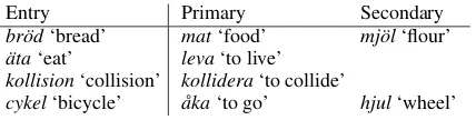
Entry Primary Secondary

br¨od‘bread’ mat‘food’ mj¨ol‘flour’

¨ata‘eat’ leva‘to live’

kollision‘collision’ kollidera‘to collide’

cykel‘bicycle’ ˚aka‘to go’ hjul‘wheel’ When using SALDO in the algorithm described in Section 2, we need to define a set of neigh-bors ni jk for every sense si j, as well as weights

wi jk corresponding to the neighbors. We defined the neighbors to be the primary descriptor and in-verse primaries (the senses for whichsi jis the pri-mary descriptor); we excluded neighbors that did not have the same part-of-speech tag assi j. The secondary descriptors were not used. For instance, br¨od has the primary descriptormat, and a large set of inverse primaries mostly describing kinds (e.g. r˚agbr¨od‘rye bread’) or shapes (e.g. limpa ‘loaf’) of bread. The neighborhood weights were set so that the primary descriptor and the set of inverse primaries were balanced: e.g. 1 for mat and 1/N if there wereN inverse primaries. After computing all the weights, we normalized them so that their sum was 1. We additionally considered a number of further heuristics to build the neighbor-hood sets, but they did not seem to have an effect on the end result.

5 Inspection of predominant senses of highly ambiguous words

Before evaluating the full WSD system in Sec-tion 6, we carry out a qualitative study of the mix variables computed by the algorithm described in Section 2. Determining which sense of a word is the most common one gives us a strong baseline for word sense disambiguation which is often very hard to beat in practice (Navigli, 2009). McCarthy et al. (2007) presented a number of methods to find the predominant word sense in a given corpus.

In Section 2, we showed how the embedding of a lemma is decomposed into a mix of sense em-beddings. Intuitively, if we assume that the mix variables to some extent correspond to the occur-rence probabilities of the senses, they should give us a hint about which sense is the most frequent one. For instance, in Figure 1 the embedding of the lemma rock is closer to that of the second sense (‘rock music’) than to that of the first sense (‘coat’), because the music sense is more frequent. For each lemma, we estimated the predominant sense by selecting the sense for which the corre-sponding mix variable was highest. To create a dataset for evaluation, an annotator selected the

most polysemous verbs, nouns, adjectives, and ad-verbs in SALDO (25 of each class) and determined the most frequent sense by considering a random sample of the occurrences of the lemma. Table 1 shows the accuracies of the predominant sense selection for all four word classes, as well as the average polysemy for each of the classes.

Part of speech Accuracy Avg. polysemy

Verb 0.48 6.28

Noun 0.76 6.12

Adjective 0.76 4.24

Adverb 0.84 2.20

Overall 0.71 4.71

Table 1: Predominant sense selection accuracy. For nouns, adjectives, and adverbs, this heuris-tic works quite well. However, similar to what was seen by McCarthy et al. (2007), verbs are the most difficult to handle correctly. In our case, this has a number of reasons, not primarily that this is the most polysemous class. First of all, the most fre-quent verbs, which we evaluate here, often partici-pate in multi-word units such as particle verbs and in light verb constructions. While SALDO con-tains information about many multi-word units, we have not considered them in this study since our preprocessing step could not deterministically extract them (as described in Section 4). Secondly, we have noticed that the sense embedding process has a problem with verbs where the sense distinc-tion is a distincdistinc-tion between transitive and intran-sitive use, e.g. koka ‘to boil’. This is because the transitive and intransitive senses typically are neighbors in the SALDO network, so their context sets will be almost identical and the algorithm will try to minimize the distance between them. 6 WSD evaluation

To evaluate our new WSD system, we applied it to two test sets and first compared it to a num-ber of baselines, and finally to UKB, a well-known graph-based WSD system.

Our two test sets were the SALDO examples (SALDO-ex)7 and the Swedish FrameNet exam-ples(SweFN-ex)8. Both resources consist of sen-tences selected by lexicographers for illustration of word senses. At the time of our experiments, SALDO-ex contained 4,489 sentences. In each

sentence, one of the tokens (the target word) has been marked up by a lexicographer and assigned a SALDO sense. SweFN-ex contained 7,991 sen-tences, and as in SALDO-ex the annotation con-sists of disambiguated target words: the differ-ence is that instead of a SALDO sense, the tar-get word is assigned a FrameNet frame (Fill-more and Baker, 2009). However, using the Swedish FrameNet lexicon (Friberg Heppin and Toporowska Gronostaj, 2012), frames can in most cases be deterministically mapped to SALDO senses: for instance, the first SALDO sense of the nounstam(‘trunk’ or ‘stem’) belongs to the frame PLANT SUBPART, while the second sense (‘tribe’) is in the frame AGGREGATE.

We preprocessed these two test sets using Spr˚akbanken’s annotation services9 to tokenize, compound-split, and lemmatize the texts and to determine the set of possible senses in a given con-text. All unambiguous instances were removed from the sets, and we also excluded sentences where the target consisted of more than one word. We then ended up with 1,177 and 1,429 instances in SALDO-ex and SweFN-ex, respectively. Figure 2 shows the distribution of the number of senses for target word in the combination of the two sets.

2 4 6 8 10 12

Polysemy 0

200 400 600 800 1000 1200 1400 1600

Frequency

Figure 2: Histogram of the number of senses for target words in the test sets.

6.1 Comparison to baselines

We applied the contextual WSD method defined by Eq. 2 to the two test sets. As the simplest base-line, we used a random selection. A much more

9_{http://spraakbanken.gu.se/korp/}

annoteringslabb/

difficult baseline is to select the first sense10in the inventory; this baseline is often very hard to beat for WSD systems (Navigli, 2009). Furthermore, we evaluated a simple approach that selects the sense whose value of the mix variable in Section 2 is highest. Table 2 shows the result.

System SALDO-ex SweFN-ex

Random 39.3 40.3

Sense 1 52.5 53.5

By mix variables 47.6 53.9

Contextual WSD 62.7 63.3

Table 2: Comparison to baselines.

We see that our WSD system clearly outperforms not only the trivial but also the first-sense baseline. Selecting the sense by the value of the mix vari-able (which can be regarded as a prior probability) gives a result very similar to the first-sense base-line: this can be useful in sense inventories where senses are not ranked by frequency or importance. (This result is lower in SALDO-ex, which is heav-ily dominated by verbs; as we saw in Section 5, the mix variables seem less reliable for verbs.) 6.2 Analysis by part of speech

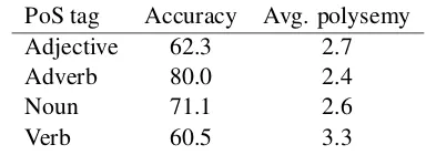
The combined set of examples from SALDO-ex and SweFN-ex contains 1,723 verbs, 575 nouns, 287 adjectives, and 15 adverbs. We made a break-down of the result by the part of speech of the tar-get word, and we show the result in Table 3.

PoS tag Accuracy Avg. polysemy

Adjective 62.3 2.7

Adverb 80.0 2.4

Noun 71.1 2.6

Verb 60.5 3.3

Table 3: Results for different parts of speech. Again, we see that verbs pose the greatest dif-ficult for our methods, while disambiguation ac-curacy is higher for nouns. Adjectives are also difficult to handle, with an accuracy just slightly higher than what we had for the verbs. (There are too few adverbs to allow any reliable conclusion to be drawn about them.) To some extent, the dif-ferences in accuracy might be expected to be cor-related with the degree of polysemy, but there are

10_{Unlike in WordNet, SALDO’s senses are not explicitly}

also other factors involved, such as the structure of the SALDO network. We leave an investigation of the causes of these differences to future work. 6.3 Comparison to graph-based WSD

To find a more challenging comparison than the baselines, we applied the UKB system, a WSD system based on personalized PageRank in the sense graph, which has achieved a very compet-itive result for a system without any annotated training data (Agirre and Soroa, 2009). Because of limitations in the UKB software, the test sets are slightly smaller (1,055 and 1,309 instances, re-spectively), since we only included test instances where the lemmas could be determined unambigu-ously. The result is presented in Table 4. This ta-ble also includes the result of a combined system where we simply added Eq. 2 to the log of the probability output by UKB.

System SALDO-ex SweFN-ex

Contextual WSD 64.0 64.2

UKB 61.2 61.2

Combined 66.4 66.0

Table 4: Comparison to the UKB system. Our system outperforms the UKB system by a slight margin; while the difference is not statisti-cally significant, the consistent figures in the two evaluations suggest that the results reflect a true difference. However, in both evaluations, the com-bination comes out on top, suggesting that the two systems have complementary strengths.

Finally, we note that our system is much faster: UKB processes the SweFN-ex set in 190 seconds, while our system processes the same set in 450 milliseconds, excluding startup time.

7 Conclusion

We have presented a new method for word sense disambiguation derived from the skip-gram model. The crucial step is to embed a semantic network consisting of linked word senses into a continuous-vector word space. Unlike previous approaches for creating vector-space representa-tions of senses, and due to the fact that we rely on the network structure, we can create represen-tations for senses that occur very rarely in corpora. Once the senses have been embedded in the vector space, deriving a WSD model is straightforward. The word sense embedding algorithm (Johansson

and Nieto Pi˜na, 2015) takes a set of embeddings of lemmas, and uses them and the structure of the semantic network to induce the sense representa-tions. It hinges on two ideas: 1) that sense embed-dings should preserve the structure of the semantic network as much as possible, i.e. that two senses should be close geometrically if they are neighbors in the graph, and 2) that lemma embeddings can be decomposed into separate sense embeddings.

We applied the sense embedding algorithm to the senses of SALDO, a Swedish semantic net-work, and a vector space trained on a large Swedish corpus. These vectors were then used to implement a WSD system, which we evaluated on two new test sets annotated with SALDO senses. The results showed that our new WSD system not only outperforms the baselines, but also UKB, a high-quality graph-based WSD implementation. While the accuracies were comparable, our system is several hundred times faster than UKB.

Furthermore, we carried out a qualitative in-spection of the mix variables estimated by the em-bedding algorithms and found that they are rela-tively good for predicting the predominant word senses: more so for nouns, adjectives and adverbs, less so for verbs. This result is consistent with what we saw in the quantitative evaluations, where selecting a sense based on the mix variable gave an accuracy similar to the first-sense baseline.

In future work, we will carry out a more sys-tematic evaluation of the word sense disambigua-tion system in several languages. For Swedish, a more large-scale evaluation requires an annotated corpus, which will give more reliable quality esti-mates than the lexicographical examples we have used in this work. Fortunately, a 100,000-word multi-domain corpus of contemporary Swedish is currently being annotated on several linguistic lev-els in the KOALA project (Adesam et al., 2015), including word senses as defined by SALDO. Acknowledgments

References

Yvonne Adesam, Gerlof Bouma, and Richard Johans-son. 2015. Defining the Eukalyptus forest – the Koala treebank of Swedish. InProceedings of the 20th Nordic Conference of Computational Linguis-tics, Vilnius, Lithuania.

Eneko Agirre and Aitor Soroa. 2009. Personalizing PageRank for word sense disambiguation. In Pro-ceedings of the 12th Conference of the European Chapter of the ACL (EACL 2009), pages 33–41, Athens, Greece.

Lars Borin, Markus Forsberg, and Lennart L¨onngren. 2013. SALDO: a touch of yin to WordNet’s yang. Language Resources and Evaluation, 47(4):1191– 1211.

Ronan Collobert and Jason Weston. 2008. A unified architecture for natural language processing: Deep neural networks with multitask learning. In Pro-ceedings of the 25th International Conference on Machine Learning, pages 160–167.

Katrin Erk and Sebastian Pad´o. 2010. Exemplar-based models for word meaning in context. InProceedings of the ACL 2010 Conference Short Papers, pages 92–97, Uppsala, Sweden.

Christiane Fellbaum, editor. 1998. WordNet: An elec-tronic lexical database. MIT Press.

Charles J. Fillmore and Collin Baker. 2009. A frames approach to semantic analysis. In B. Heine and H. Narrog, editors, The Oxford Handbook of Lin-guistic Analysis, pages 313–340. Oxford: OUP.

Karin Friberg Heppin and Maria Toporowska Gronos-taj. 2012. The rocky road towards a Swedish FrameNet – creating SweFN. InProceedings of the Eighth conference on International Language Re-sources and Evaluation (LREC-2012), pages 256– 261, Istanbul, Turkey.

Amaru Cuba Gyllensten and Magnus Sahlgren. 2015. Navigating the semantic horizon using relative neighborhood graphs. CoRR, abs/1501.02670.

Zellig Harris. 1954. Distributional structure. Word, 10(23).

Eric H. Huang, Richard Socher, Christopher D. Man-ning, and Andrew Y. Ng. 2012. Improving word representations via global context and multiple word prototypes. InAssociation for Computational Lin-guistics 2012 Conference (ACL 2012), Jeju Island, Korea.

Richard Johansson and Luis Nieto Pi˜na. 2015. Embed-ding a semantic network in a word space. In Pro-ceedings of the 2015 Conference of the North Amer-ican Chapter of the Association for Computational Linguistics – Human Language Technologies, Den-ver, United States.

Mikael K˚ageb¨ack, Fredrik Johansson, Richard Johansson, and Devdatt Dubhashi. 2015. Neural context embeddings for automatic discovery of word senses. In Proceedings of the Workshop on Vector Space Modeling for NLP, Denver, United States. To appear.

Pentti Kanerva, Jan Kristoffersson, and Anders Holst. 2000. Random indexing of text samples for latent semantic analysis. InProceedings of the 22nd An-nual Conference of the Cognitive Science Society.

Thomas K. Landauer and Susan T. Dumais. 1997. A solution to Plato’s problem: The latent seman-tic analysis theory of acquisition, induction and rep-resentation of knowledge. Psychological Review, 104:211–240.

Omer Levy and Yoav Goldberg. 2014. Linguistic regularities in sparse and explicit word representa-tions. In Proceedings of the Eighteenth Confer-ence on Computational Natural Language Learning, pages 171–180, Ann Arbor, United States.

Diana McCarthy, Rob Koeling, Julie Weeds, and John Carroll. 2007. Unsupervised acquisition of pre-dominant word senses. Computational Linguistics, 33(4):553–590.

Tom´aˇs Mikolov, Kai Chen, Greg Corrado, and Jeffrey Dean. 2013a. Efficient estimation of word repre-sentations in vector space. InInternational Confer-ence on Learning Representations, Workshop Track, Scottsdale, USA.

Tom´aˇs Mikolov, Ilya Sutskever, Kai Chen, Greg Cor-rado, and Jeff Dean. 2013b. Distributed representa-tions of words and phrases and their compositional-ity. InAdvances in Neural Information Processing Systems 26.

Tom´aˇs Mikolov, Wen-tau Yih, and Geoffrey Zweig. 2013c. Linguistic regularities in continuous space word representations. InProceedings of the 2013 Conference of the North American Chapter of the Association for Computational Linguistics: Human Language Technologies, pages 746–751, Atlanta, USA.

Andriy Mnih and Koray Kavukcuoglu. 2013. Learning word embeddings efficiently with noise-contrastive estimation. InAdvances in Neural Information Pro-cessing Systems 26, pages 2265–2273.

Hans Moen, Erwin Marsi, and Bj¨orn Gamb¨ack. 2013. Towards dynamic word sense discrimination with random indexing. InProceedings of the Workshop on Continuous Vector Space Models and their Com-positionality, pages 83–90, Sofia, Bulgaria.

Roberto Navigli. 2009. Word sense disambiguation: a survey. ACM Computing Surveys, 41(2):1–69.

per word in vector space. In Proceedings of the 2014 Conference on Empirical Methods in Natural Language Processing (EMNLP), pages 1059–1069, Doha, Qatar.

Sebastian Pad´o and Mirella Lapata. 2007. Dependency-based construction of semantic space models. Computational Linguistics, 33(1).

Fabian Pedregosa, Ga¨el Varoquaux, Alexandre Gram-fort, Vincent Michel, Bertrand Thirion, Olivier Grisel, Mathieu Blondel, Peter Prettenhofer, Ron Weiss, Vincent Dubourg, Jake VanderPlas, Alexan-dre Passos, David Cournapeau, Matthieu Brucher, Matthieu Perrot, and Edouard Duchesnay. 2011. Scikit-learn: Machine learning in Python. Journal of Machine Learning Research, 12:2825–2830.

Amruta Purandare and Ted Pedersen. 2004. Word sense discrimination by clustering contexts in vector and similarity spaces. InHLT-NAACL 2004 Work-shop: Eighth Conference on Computational Natu-ral Language Learning (CoNLL-2004), pages 41– 48, Boston, United States.

Magnus Sahlgren. 2006. The Word-Space Model. Ph.D. thesis, Stockholm University.

Hinrich Sch¨utze. 1998. Automatic word sense dis-crimination. Computational Linguistics, 24(1):97– 123.

Joseph Turian, Lev-Arie Ratinov, and Yoshua Bengio. 2010. Word representations: A simple and gen-eral method for semi-supervised learning. In Pro-ceedings of the 48th Annual Meeting of the Associa-tion for ComputaAssocia-tional Linguistics, pages 384–394, Uppsala, Sweden.