Karst Network
By
Ted McCormack B.Eng., MSc., PG Dip. Stat.
A Thesis submitted to the University of Dublin for the degree of
Doctor of Philosophy
Department of Civil, Structural and Environmental Engineering
University of Dublin
as an exercise for a degree at this or any other university.
I also give the library permission to lend or copy this thesis, upon request, for academic purposes. This permission covers only single copies made for study purposes, subject to normal conditions of acknowledgment.
_____________
In this thesis, hydrochemical methods are used in combination with hydrologic analysis to characterise and model the Gort Lowlands catchment in western Galway, specifically focussing on an interlinked chain of ephemeral lakes (known as turloughs). The Gort Lowlands is a relatively unique karstic system, both hydrologically and hydrochemically, and lies within the pure Carboniferous lowlands of western Ireland. The primary source of water to the catchment is derived from the largely impermeable Devonian sandstone catchment found on the Slieve Aughty Mountains. Three rivers draining from these mountains (the Owenshree, Ballycahalan and Beagh Rivers) discharge down into the karst lowlands allogenically, imparting the catchment with a distinct hydrochemical flux.
The Gort Lowlands catchment has been monitored and sampled for over three years, focussing on five turloughs in particular, Blackrock, Coy, Coole, Garryland and Caherglassaun. These turloughs form an interlinked chain, joined by subterranean conduits which ultimately drain at a series of intertidal springs at Kinvara. The turloughs are known to act as surcharge tanks, filling with excess water when the underground conduit network has reached capacity. Over the study period, these turloughs as well as rivers, groundwater and outlet springs were sampled monthly in an effort to characterise the hydrochemical behaviour of the entire catchment. The hydrologic behaviour of the karst lowlands was found to be dominated by an active conduit network. This network is fed by the Beagh, Owenshree and Ballycahalan Rivers which contribute 55.3%, 24% and 20.7% of the total flow respectively. The flow through this conduit network is supplemented by input from the epikarst system which surrounds it. Hydrochemical and modelling studies found this epikarstic contribution to add approximately 10-17% extra flow to the system.
very similar concentrations to their feeding river whereas the lower three turloughs displayed higher alkalinity concentrations, most likely due to the contribution of high alkalinity water from the epikarst as water moved through the system. Using alkalinity and EC measurements, the contrasting water retention behaviour of the turloughs was investigated. Blackrock and Coole turloughs both exhibit flow-through behaviour whereas Coy and Caherglassaun present surcharge tank behaviour. The behaviour of Garryland changes depending on water level; at lower water levels, it acts as a surcharge tank and at higher water levels, it hydraulically joins with Coole and acts more like a flow-through system. Alkalinity measurements also showed an influx of diffuse groundwater into the turloughs over the flooding season, particularly during a recession period. The volume of water entering the turloughs amounted to between 1 and 10% of the entire volume that drained from a turlough during a recession period.
Analysis of nutrient concentrations (nitrogen, N, and phosphorus, P) within the catchment found that as water moves through the conduit network, it gains N and loses P. The gain in N is due to contribution from the N-enriched epikarst. As a result of this enrichment, the N load at the tidal spring at Kinvara was shown to be approximately 17% higher than that of the combined river input into the system. This load is lower than would be expected (based on model results) due to N losses within the turloughs. It was postulated that the primary mechanism of N loss within the turloughs was denitrification. Unlike N, P loads decrease as water moves through the system. The P load discharging at Kinvara was found to be approximately 8% lower than the combined input from the rivers. This reduction was due to the minimal contribution of P from the epikarst and P losses from the turloughs. The primary mechanism of P loss within the turloughs was deemed to be sedimentation. Overall, the turloughs appear to act as nutrient sinks over flooded periods, particularly the surcharge tank turloughs. Blackrock and Coy turloughs, however, were found to be nutrient sources, primarily due to the presence of an abattoir at Blackrock (enhancing N and P) and a high degree of grazing during dry periods (enhancing P).
Firstly, I would like to express my thanks to Dr. Laurence Gill for supervising me throughout this thesis. Laurence has been there throughout my PhD research to offer valuable advice and constructive suggestions, whether it came to numerical modelling advice or chain-sawing tree stumps out of rivers, Laurence’s hands-on approach to project supervision was extremely helpful and often entertaining.
Thank you to my co-supervisor Professor Paul Johnston for his guidance over the course of this project and the effort he put into acquiring my project funding.
I wish to acknowledge the AXA Research Fund for providing the funding that enabled me to undertake this research project.
I wish to thank Owen Naughton for being smarter than me about all things karst, and to Pat Veale for his help with fieldwork and laboratory testing.
I would like to thank my fellow Pearse Street office dwellers, Aisling, Andy, Davie, Francesco, John, Mairead, Seanie and the Commissioner. Four years in Pearse Street has been a true experience and a stunning performance. I fear I shall never again be part of an office of such high calibre nonsense.
I would also like to thank all those who helped me with site work over the years. In particular, I wish to thank Laura, Maurice and Maeve for their contribution.
I would like to thank Aisling, for putting up with me both in the office and out of it. I look forward to the chocolate biscuit cake you have promised me when this is all over.
Declaration ... i
Summary ... ii
Acknowledgements ... iv
List of Figures ... xi
List of Tables ... xxi
Abbreviations ... xxiii
1
Introduction ... 3
1.1 Background ... 3
1.2 Aims and objectives... 4
2
Literature review... 9
2.1 Overview of Karst Hydrology ... 9
2.2 Karst Aquifers ... 10
2.2.1 Recharge ... 12
2.2.2 Flow Systems ... 14
2.2.3 Discharge ... 17
2.2.4 Chemistry... 18
2.3 Karst Network Development ... 20
2.3.1 Energy Supply ... 20
2.3.2 Fracture Enlargement ... 21
2.3.3 Development of Vadose Zone and Epikarst ... 22
2.3.4 Conduit Network Development ... 24
2.4 Investigative Techniques ... 26
2.4.1 Geomorphology and Speleology ... 26
2.4.2 Boreholes and Test Wells ... 27
2.4.3 Geophysical Methods ... 28
2.4.4 Artificial Tracers ... 31
2.4.5 Environmental Tracers (Isotopes) ... 34
2.4.6 Spring Hydrographs ... 37
2.4.7 Spring Water Chemistry (Hydrochemistry) ... 39
2.5 Modelling Karst Aquifers ... 43
3
Background and Site Description ... 57
3.1 Irish Karst ... 57
3.2 The Gort Lowlands: Geology and Hydrogeology ... 59
3.3 Speleological Investigations ... 66
3.4 Turloughs ... 70
3.4.1 Definition and Origin ... 70
3.4.2 Distribution ... 71
3.4.3 Turlough Hydrology ... 73
3.4.4 Turlough Ecology ... 75
3.5 Previous Hydrological Studies in the Gort Lowlands ... 83
3.5.1 Gort Flood Studies ... 84
3.5.2 Review of Gort Flood Studies and Proposed Engineering Works ... 88
3.6 Gort Lowland Turlough Network ... 92
3.6.1 Blackrock turlough ... 92
3.6.2 Coy turlough... 93
3.6.3 Coole turlough... 95
3.6.4 Garryland turlough ... 96
3.6.5 Caherglassaun turlough ... 97
3.7 Summary ... 99
4
Instrumentation and Data Collection ... 103
4.1 Introduction ... 103
4.2 Continuous Monitoring ... 103
4.2.1 Turlough Water Levels ... 104
4.2.2 Groundwater Levels ... 105
4.2.3 Rainfall ... 107
4.2.4 River Gauging ... 107
4.3 Monthly Sampling ... 111
4.4 External Data ... 114
4.5 Chemical Analysis ... 115
4.5.1 General Chemistry ... 115
4.5.2 Nutrients ... 116
4.5.3 Stable Isotopes ... 117
5.2 Turloughs ... 123
5.2.1 Updating Turlough Surveys ... 126
5.3 Rainfall & Evapotranspiration ... 128
5.3.1 Rainfall ... 128
5.3.2 Evapotranspiration ... 131
5.4 Rivers ... 131
5.4.1 Rating Curves ... 132
5.4.2 Rainfall-Runoff Modelling... 136
5.4.3 Analysis ... 140
5.5 Groundwater ... 143
5.6 Tide ... 150
6
Pipe Network Modelling ... 155
6.1 Introduction ... 155
6.2 Physical Model: ... 155
6.2.1 Results ... 158
6.2.2 Effect of Bypass ... 160
6.2.3 Effect of Inlet Constriction ... 160
6.2.4 Effect of Throttles ... 162
6.2.5 Effect of River Input ... 164
6.2.6 Tracer Studies ... 166
6.2.7 Physical Model Conclusions ... 171
6.3 Gort Lowlands Infoworks Model ... 172
6.3.1 Infoworks CS ... 172
6.3.2 Gort Lowlands Model ... 173
6.3.3 Recalibration ... 180
6.3.4 Model Analysis – Model Parameters ... 195
6.4 Evaluating the Impact of Climate Change using the Pipe-Network Model. ... 201
6.4.1 Global Trends ... 201
6.4.2 Climate Change in Ireland... 203
6.4.3 Application of the Gort Lowlands Model ... 204
6.4.4 Results ... 208
6.5 Water Quality Modelling ... 218
7.1.2 Land Use and Associated Nutrients/Contamination ... 227
7.1.3 Previous Studies and Findings ... 231
7.2 Alkalinity, pH, and Electrical Conductivity ... 234
7.2.1 Results of Monthly Sampling ... 235
7.2.2 Quantifying Diffuse Input using CTD Divers... 247
7.2.3 CTD Study of Blackrock and Coy turloughs ... 251
7.2.4 CTD Study of Kinvara Bay ... 260
7.3 Nutrients ... 268
7.3.1 Results ... 269
7.4 Nutrient Modelling ... 291
7.4.1 Turlough Nutrient Retention. ... 291
7.4.2 Diffuse Contribution... 301
7.4.3 Water Quality Modelling - Discussion ... 303
7.5 Discussion ... 304
7.5.1 Hydrochemical behaviour across the catchment ... 305
7.5.2 Hydrochemical Behaviour within turloughs ... 307
7.6 Ballinduff ... 316
8
Stable Isotopes of water,
18O and
2H ... 323
8.1 Background ... 323
8.2 Isotopes in Precipitation... 327
8.3 Isotopes in Surface water and Groundwater ... 332
8.3.1 Rivers ... 336
8.3.2 Turloughs ... 339
8.3.3 Groundwater ... 345
8.3.4 Kinvara ... 347
8.4 Discussion ... 350
9
Conclusions ... 355
9.1 Conclusions... 355
9.2 Recommendations for Further Research ... 362
Figure 2.1: Global distribution of major outcrops of carbonate rocks (dark blue: pure, continuous,
light blue: impure, discontinuous) (Williams and Ford, 2006) ... 9
Figure 2.2: Conceptual model for a carbonate aquifer (White, 2002) ... 11
Figure 2.3: Illustration displaying duality of recharge (allogenic vs. autogenic) and infiltration (point vs. diffuse) (Goldscheider and Drew, 2007)... 13
Figure 2.4: Estavelle at Coy Turlough. Acting as sink in summer (a) and a spring in winter (b) ... 18
Figure 2.5: Relationship between soil CO2, rate of limestone solution and fissuring beneath the soil. (Williams, 1983) ... 23
Figure 2.6: Resistivity study of Caherglassaun turlough (overlaid with topography plot), (O'Connell et al., 2012). ... 30
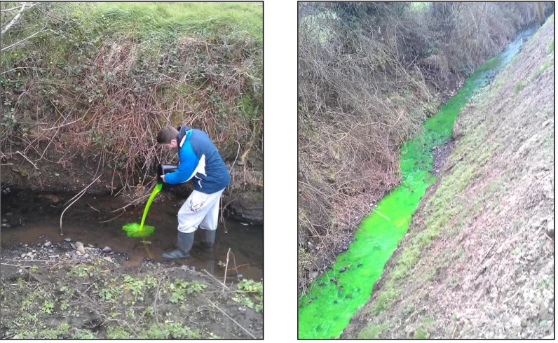
Figure 2.7: Injection of uranine dye into a small stream. ... 32
Figure 2.8: Tracer tests in the Gort Lowlands catchment carried out as part of the Gort Flood Studies Report (Drew, 2003). ... 34
Figure 2.9: Hydrological and isotopic budget of a lake system (Mook, 2001) ... 36
Figure 2.10: Storm hydrograph from Big Spring MO, showing quickflow ... 38
Figure 2.11: Piston flow behaviour in Coy turlough, January 2013. Blue line is EC, Black line is Stage. ... 41
Figure 2.12: Double fissured porosity system (Drogue, 1980) ... 44
Figure 2.13: Conceptual model of Fontaine de Vacluse system (Fleury et al., 2007) ... 47
Figure 2.14: Classification of distributive karst modelling methods (Kovacs and Sauter, 2007) ... 48
Figure 2.15: DCN model of downstream part of Hölloch cave (Jeannin, 2001) ... 50
Figure 3.1: Distribution of carboniferous limestone in Ireland (Drew, 2008). ... 57
Figure 3.2: Map of Gort lowlands showing the locations of turloughs, rivers, lakes, springs, swallow holes and towns. ... 60
Figure 3.3: East-West sketch section through the Burren and Gort Lowlands (Simms, 2001). The location of the section X-X can be seen in Figure 3.4 ... 61
Figure 3.4: Bedrock geology of the Gort Lowlands ... 61
Figure 3.5: Ballylee sink north discharging (A) and empty (B). ... 63
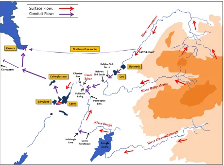
Figure 3.6: Schematic map displaying the distribution of flow within the Gort Lowlands. ... 66
Figure 3.7: Map displaying locations of speleological sites of interest and explored cave systems (red lines). ... 67
Figure 3.10: Flow-through and surcharge tank conceptualisations of turloughs (Naughton, 2011). . 75
Figure 3.11: Horses grazing at Coy turlough. ... 82
Figure 3.12: Flooding at Kiltartan, November 2009 (Jennings O'Donovan & Partners, 2011). ... 84
Figure 3.13: Groundwater level contour maps showing the hydraulic gradient of the catchment during March and April 1997 (based on the maps of Southern Water Global (1998)) ... 86
Figure 3.14: Locations of proposed engineering works as part of the Gort Flood Studies Review (Jennings O'Donovan & Partners, 2011). ... 91
Figure 3.15: Blackrock turlough, summer vs. winter. ... 93
Figure 3.16: Coy turlough, summer vs. winter. ... 94
Figure 3.17: Coole turlough, summer vs. winter. ... 95
Figure 3.18: Garryland turlough, summer vs. winter. ... 96
Figure 3.19: Caherglassaun turlough, summer vs. winter. ... 97
Figure 3.20: Caherglassaun turlough water levels and Kinvara tidal variation (Gill et al., 2013b). ... 98
Figure 4.1: Monitoring locations (measuring water depth or rainfall). ... 104
Figure 4.2: Diver platform, site laptop, diver download cable and various diver models. ... 105
Figure 4.3: Various groundwater access points within the catchment. ... 106
Figure 4.4: Francis Gap rain gauge. ... 107
Figure 4.5: OPW River gauging station showing pressure transducer and staff gauge. ... 108
Figure 4.6: Measuring river flow. ... 109
Figure 4.7: ADC meter used to measure flow. ... 109
Figure 4.8: Low flow and high flow (8/6/2012) comparison at Owendalulleegh River. ... 110
Figure 4.9: Measuring high flows on Ballycahalan River (8/612). ... 110
Figure 4.10: Plot of sampling network displaying site type (colour) and name. ... 112
Figure 5.1: Turlough water levels (stage) for all turloughs, daily rainfall from Francis Gap rain gauge ... 124
Figure 5.2: Blackrock turlough ... 128
Figure 5.3: Blackrock turlough LIDAR updated survey. ... 128
Figure 5.4: Upgraded stage-volume curve for Blackrock turlough. ... 128
Figure 5.5: Daily rainfall correlation between Kilchreest and Francis Gap (Sep 2010-April 2013). .. 129
Figure 5.6: Monthly rainfall for Kilchreest rain gauge (2010-2013). ... 129
Figure 5.7: Rainfall contour map for the Gort Lowlands (Office of Public Works, 2013)... 130
Figure 5.8: PE data used for the Gort Lowlands. ... 131
Figure 5.12: Ballycahalan rating curve. ... 134
Figure 5.13: Owendalulleegh River rating curve. ... 135
Figure 5.14: Beagh River rating curve. ... 136
Figure 5.15: NAM conceptual structure (from O’Brien et al. (2013)). ... 137
Figure 5.16: Example of observed (blue) & predicted (red) runoff for Kilchreest River ... 139
Figure 5.17: Owenshree River hydrograph with NAM flow estimations. ... 140
Figure 5.18: Cumulative flow for Owenshree, Ballycahalan and Beagh Rivers ... 141
Figure 5.19: Lough Cutra and its feeding/receiving rivers... 142
Figure 5.20: Owendalulleegh inflow and Beagh outflow from Lough Cutra. ... 142
Figure 5.21: Owenshree flow & Blackrock turlough level (August-October 2012). Red circles indicate periods when flow exceeds 1.23m3/h and thus causes a response from the turlough. ... 143
Figure 5.22: Various degrees of borehole water level fluctuation within the catchment. Solid line represents continuous monitoring using a diver. Points and dotted line represent point measurements and interpolation. ... 144
Figure 5.23: Borehole locations in this study superimposed upon groundwater level fluctuations as mapped out by the Gort Flood Studies (Southern Water Global, 1998). ... 145
Figure 5.24: BH3 & Blackrock turlough water levels (Feb 2011-Mar 2013). ... 146
Figure 5.25 BH3 water level & Owenshree flow (Apr-Sept 2012). ... 146
Figure 5.26: BH7 & Blackrock turlough water levels (Jun 2010-Mar 2013). ... 147
Figure 5.27: BH17 & Coy turlough water levels (Aug 2010-Jun 2011). ... 147
Figure 5.28: BH12 & Coole turlough water levels (May 2010–Aug 2012). ... 148
Figure 5.29: Non-Responsive boreholes/wells water levels (Jan 2010 – May 2013). ... 148
Figure 5.30: BH14 (small scale) and Blackrock turlough comparison. ... 149
Figure 5.31: BH20 and Coole turlough water levels (August 2010 – May 2013). ... 149
Figure 5.32: BH15 and Coy turlough water levels (May 2010 – April 2012). ... 150
Figure 5.33: Tidal data for Galway city and Kinvara. Note the 72 minute offset between the two locations. ... 150
Figure 6.1: Blackrock-Coy conceptualisation from Gill (2010). ... 156
Figure 6.2: Photo of physical model. ... 156
Figure 6.3: Physical model schematic. ... 157
Figure 6.4: Tap valves underneath the Upper Turlough (UT). ... 159
Figure 6.5: Input signal 1. ... 159
Figure 6.9: Constricting UT inlet (UT). ... 161
Figure 6.10: Constricting UT inlet (LT)... 161
Figure 6.11: Constricting LT inlet (UT)... 161
Figure 6.12: Constricting LT inlet (LT). ... 161
Figure 6.13: Constricting both inlets (UT). ... 161
Figure 6.14: Constricting both inlets (LT). ... 161
Figure 6.15: Constricting UT throttle (UT). ... 162
Figure 6.16: Constricting UT throttle (LT). ... 162
Figure 6.17: Constricting LT throttle (UT). ... 163
Figure 6.18: Constricting LT throttle (LT). ... 163
Figure 6.19: Constricting both throttles (UT)... 163
Figure 6.20: Constricting both throttles (LT). ... 163
Figure 6.21: Coy bypass and throttle combination (UT). ... 164
Figure 6.22: Coy bypass and throttle combination (LT)... 164
Figure 6.23: River-Conduit test results. ... 165
Figure 6.24: Fluorescein injection using syringe. ... 167
Figure 6.25: Tank containing fluorescein. ... 167
Figure 6.26: Tracer test – River input. ... 167
Figure 6.27: Tracer test – Conduit input. ... 168
Figure 6.28: Tracer test – Conduit input, bypass closed. ... 168
Figure 6.29: Tracer test – Conduit input, bypass open. ... 169
Figure 6.30: Tracer test – Split river/conduit input, bypass closed... 169
Figure 6.31: Tracer test – Split river/conduit input, bypass open. ... 169
Figure 6.32: Tracer test – Split river/conduit input, throttles applied, bypass closed. ... 170
Figure 6.33: Tracer test – Split river/conduit input, throttles applied, bypass open. ... 170
Figure 6.34: Conceptual model of the Gort Lowlands (Gill et al., 2013a, Gill et al., 2013b). ... 174
Figure 6.35: Model Layout overlaid on topographical map. ... 174
Figure 6.36: Conceptual model of the runoff model, soil storage reservoir and groundwater store reservoir (Gill et al., 2013a). ... 175
Figure 6.37: Schematic of Gort Lowlands model as seen in Infoworks. ... 176
Figure 6.38: Blackrock and Coy results (2007-2008) from Gill et al. (2013a) model. ... 177
Figure 6.41: Newtown and Hawkhill turlough connection with Coole. ... 180
Figure 6.42: Underground conduits targeted for sensitivity analysis. ... 181
Figure 6.43: Sensitivity analysis test period (Sept – Oct 2010). ... 181
Figure 6.44: Comparison of SWMM and Infoworks simulations (with observed water level) for the analysis period (Blackrock turlough). ... 183
Figure 6.45: Sensitivity Analysis results: Volume change in Coole with conduits expanded. ... 185
Figure 6.46: Sensitivity Analysis results: Volume change in Coole with conduits narrowed. ... 185
Figure 6.47: Percentage change in volume of Coole turlough from increasing size of individual conduits by 100%. ... 186
Figure 6.48: Percentage change in volume of Coole turlough from decreasing size of individual conduit by 50%. ... 186
Figure 6.49: Flooding patterns (Blackrock). ... 188
Figure 6.50: Model schematic (new links in red) ... 188
Figure 6.51: Model schematic (Coole bypass highlighted in red). ... 189
Figure 6.52: Coole turlough updated with epiphreatic drainage. ... 190
Figure 6.53: Flooding pattern (Coole). ... 190
Figure 6.54: Model schematic (Coole-Garryland epikarst channel in red). ... 190
Figure 6.55: Flooding Patterns (Garryland). ... 190
Figure 6.56: Model Schematic (northern flow route in red). ... 191
Figure 6.57: Flooding patterns (Blackrock). ... 191
Figure 6.58: Blackrock and Coy final calibration. Note: the sudden drop of observed stage in Blackrock in April 2012 is due to diver repositioning (discussed in Section 5.2) ... 192
Figure 6.59: Coole, Garryland and Caherglassaun final calibration results. ... 193
Figure 6.60: Modelled outflow at Kinvara (July 2010 – March 2013). ... 195
Figure 6.61: Increasing roughness (Blackrock)... 196
Figure 6.62: Decreasing roughness (Blackrock). ... 196
Figure 6.63: Elliptical vs. circular conduits (Blackrock). ... 197
Figure 6.64: Input sensitivity analysis results (Blackrock). ... 200
Figure 6.65: Input sensitivity analysis results (Coole). ... 200
Figure 6.66: Projected global GHG emission scenarios until 2100 (IPCC, 2007). ... 202
Figure 6.67: Global average projections for sea level rise (from Church et al. (2011))... 205
Figure 6.68: Lough Cutra. ... 206
Figure 6.72: Turlough flooding patterns according to emission scenario A2. ... 209
Figure 6.73: Turlough flooding patterns according to emission scenario B2. ... 210
Figure 6.74: Cumulative flow plots for the Owenshree River for scenarios A2 and B2 for the period between Jan 2011 and October 2012. ... 212
Figure 6.75: Flood duration curves for each turlough for scenarios A2 and B2 over the period Jan 2011 – Jan 2012. ... 216
Figure 7.1: Scatter plots of total percentage area of grassland/agricultural land in turlough ZOCs and mean TP (c) and TN (d) per turlough (Cunha Pereira, 2011). ... 230
Figure 7.2: Locations of current and proposed wastewater outfalls at Kinvara. ... 234
Figure 7.3: Piper diagram for groundwater samples taken near Kinvara ... 235
Figure 7.4: Alkalinity and EC correlation for each hydrological system (rivers, turloughs. groundwater and Kinvara). ... 237
Figure 7.5: Time-series plots of alkalinity results for rivers. Dots represent individual samples and dashed lines are used to aid graphical interpretation. ... 238
Figure 7.6: Blackrock turlough stage and alkalinity results (September-March 2012). ... 239
Figure 7.7: Time-series plots of alkalinity and turlough stage values. Highlighted circles represent drops in alkalinity following a period of flooding. Note: ORL refers to ‘Owenshree River Lower’ 241 Figure 7.8: Conceptualisation of diffuse flow-through, river flow-through and surcharge tank turlough systems. ... 242
Figure 7.9: Suitable data points for calculating epikarst recharge (Spring 2012). ... 242
Figure 7.10: Alkalinity results for Boreholes/wells. ... 244
Figure 7.11: Alkalinity results from Kinvara springs with modelled discharge (yellow). ... 245
Figure 7.12: Alkalinity results from Kinvara West (KW) and Caherglassaun turlough. ... 246
Figure 7.13: Owenshree River gauge locations. ... 247
Figure 7.14: Flow data for Kilchreest and Castle-Daly gauging stations (May-July2013) ... 248
Figure 7.15: EC data for Kilchreest and Castle-Daly gauging stations (May-July 2013). ... 248
Figure 7.16: Owenshree River dried up at Castle-Daly gauging station (9th July 2013). ... 249
Figure 7.17: Hydrograph separation of Castle-Daly gauging station. ... 250
Figure 7.18: CTD diver locations in Blackrock and Coy turloughs. ... 252
Figure 7.19: Flow and EC data from Castle-Daly River gauge (and precipitation). ... 253
Figure 7.20: Stage and EC data from Blackrock turlough. ... 253
Figure 7.21: Stage and EC data from Coy turlough. ... 253
Figure 7.25: ERT study of Blackrock turlough (modified from O'Connell et al. (2011)). ... 256
Figure 7.26: Typical influx pattern at Coy Spring (left – EC, right – temperature). ... 257
Figure 7.27: Anomalous influx pattern at Coy Spring (left – EC, right – temperature). ... 257
Figure 7.28: EC data from the Owenshree River and Coy turlough showing piston flow behaviour (December 2012). ... 258
Figure 7.29: CTD locations in Kinvara Bay. ... 261
Figure 7.30: CTD positioning in the water... 261
Figure 7.31: Data from the spring CTD (8th July – 14th July). ... 262
Figure 7.32: Conceptual interface between saltwater and freshwater at Kinvara spring. ... 262
Figure 7.33: Data from the Midpoint CTD (3rd May – 5th May). ... 263
Figure 7.34: Data from the Outlet CTDs (water column – solid line, base – dashed line), 8th July – 14th July. ... 263
Figure 7.35: Salinity transect of Kinvara Bay at depth 10 cm. Pink line represents the path taken along the bay, yellow line represents the water’s Salinity. ... 264
Figure 7.36: Salinity transect of Kinvara Bay at depth 90 cm. Pink line represents the path taken along the bay, yellow line represents the water’s Salinity. ... 264
Figure 7.37: Freshwater wedge calculation showing time series plot (top) and conceptual plots for points A, B, C and D. ... 266
Figure 7.38: Regression plots of Flow vs TN and TP Concentrations (Owenshree River)... 271
Figure 7.39: Time-series plots of Total Nitrogen (TN) and Nitrate (NO3) results for rivers. ... 272
Figure 7.40: Time-series plots of Total Phosphorus (TP) and Total Dissolved Phosphorus (TDP) results for rivers. ... 273
Figure 7.41: Time-series plots of Total Nitrogen (TN) and Nitrate (NO3) concentrations for Blackrock, Coy, Coole. Garryland and Caherglassaun turloughs... 279
Figure 7.42: Time-series plots of Total Phosphorus (TP) and Total Dissolved Phosphorus (TDP) concentrations for Blackrock, Coy, Coole, Garryland and Caherglassaun turloughs. ... 280
Figure 7.43 Nutrient Loading of Ardkill turlough 06-07 (data from Cunha Pereira (2011)). ... 281
Figure 7.44: Nutrient Loading of Caherglassaun turlough 06-07 (data from Cunha Pereira (2011)). ... 281
Figure 7.45: Time-series plots of Total Nitrogen (TN), Nitrate (NO3) loads for Blackrock, Coy, Coole, Garryland and Caherglassaun turloughs. ... 282
Figure 7.48: Time-series plots of Total Nitrogen (TN), Nitrate (NO3), Total Phosphorus (TP) and
Total Dissolved Phosphorus (TDP) results for BH11, BH12, BH14, BH15 and BH16. ... 286
Figure 7.49: Time-series plots of Total Nitrogen (TN), Nitrate (NO3), Total Phosphorus (TP) and Total Dissolved Phosphorus (TDP) results for KW and KE. ... 288
Figure 7.50: Daily Nutrient Loads exiting the system at KW (based on modelled outflow). ... 289
Figure 7.51: Observed and modelled results for P loading from scenario 1 (constant nutrient inputs). ... 293
Figure 7.52: Observed and modelled P concentrations in the Owenshree, Ballycahalan and Owendalulleegh/Beagh Rivers (scenario 2). ... 294
Figure 7.53: Model results for P loading from scenario 2 (modelling the P plume of July 2012) ... 295
Figure 7.54: Modelled P concentration in the Owenshree, Ballycahalan and Beagh Rivers (scenario 3) ... 297
Figure 7.55: Model results for P loading scenario 3 (P-Plume occurs during a high water-level period) ... 298
Figure 7.56: Model P concentration in the Owenshree, Ballycahalan and Beagh Rivers (scenario 4). ... 299
Figure 7.57: Model results from Scenario 4 (P plume occurs at onset of flooding). ... 300
Figure 7.58: Blackrock turlough diffuse-conduit contribution comparison for Flow, NO3 and TDP (August 2010 – March 2013). ... 301
Figure 7.59: Coole turlough diffuse-conduit contribution comparison for Flow, NO3 and TDP (August 2010 – March 2013). ... 302
Figure 7.60: River-turlough NO3 comparison, (Blackrock, 2012-2013 season). ... 309
Figure 7.61: River-turlough TDP comparison, (Coole, 2012-2013 season). ... 309
Figure 7.62: Denitrification example, Caherglassaun. Denitrification occurring between points A and B. ... 312
Figure 7.63: Ballinduff location map. ... 316
Figure 7.64: Ballinduff turlough, dry vs. wet. ... 317
Figure 7.65: Hydrographs of Ballinduff and Garryland turloughs (December 2012 – July 2013). .... 317
Figure 8.1: Delta plot (18δ vs. 2δ) showing GMWL and theoretical evaporation line ... 325
Figure 8.2: Valentia measurments and LMWL (1990-2012)... 328
Figure 8.3: Gort Lowlands River data plotted with Valentia LMWL and GMWL. ... 329
Figure 8.4: Gort Lowlands river data plotted with the approximate LMWL (2δ = 6.918δ + 7‰). ... 330
Figure 8.8: Delta-plot for all surface-water samples (segregated into rivers, turloughs and KW). .. 334
Figure 8.9: Delta-plot showing LMWL and theoretical evaporation line overlaid on isotopic data. 336 Figure 8.10: 18δ values for river samples (May 2010 – December 2012). ... 337
Figure 8.11: Delta plots for river sites ORL, BRL, DRL and F. ... 338
Figure 8.12: 18δ - 2δ plot showing all rivers with atypical readings highlighted. ... 339
Figure 8.13: 18δ - d-excess plot showing all rivers with atypical readings highlighted. ... 339
Figure 8.14:Time series plots of river and turlough isotopic compositions and turlough stage for Blackrock, Coy, Coole, Garryland and Caherglassaun turloughs... 340
Figure 8.15: Net daily precipitation/evaporation (March 2010 – December 2012). ... 342
Figure 8.16: Comparison of turlough and river isotopic compositions using delta-plots and time series for the purpose of determining evaporation (Blackrock turlough, September-December 2012). ... 343
Figure 8.17: Delta plots showing evaporation influenced samples for each turlough individually and a group plot. ... 344
Figure 8.18: Delta plot of groundwater. ... 345
Figure 8.19: Time series plots of 18δ in groundwater. ... 346
Figure 8.20: 18δ verses depth of sample from surface. ... 347
Figure 8.21: Time series plot of Caherglassaun and Kinvara West (KW). ... 348
Figure 8.22: Delta plots of Kinvara West (KW) and Kinvara East (KE). ... 349
Figure 8.23: Time series plot of 18δ at Kinvara West (KW) and Kinvara East (KE). ... 349
Figure 9.1: Synthetic sketch displaying the relationship between the various elements of this thesis. ... 355
18O Oxygen 18 isotope
2H Deuterium isotope
ANC Acid Neutralisation Capacity
CDC Combined Discrete-Continuum Approach CIFR Conduit-Influenced Flow Regime
DC Double Continuum Approach
DCN Discrete Channel Network Approach DFN Discrete Fracture Network approach DIP Dissolved Inorganic Phosphorous
DO Dissolved Oxygen
DOP Dissolved Organic Phosphorous EC Electrical Conductivity
EMMA End Member Mixing Analysis EPA Environmental Protection Agency EPM Equivalent Porous Medium Approach ERT Electrical resistivity tomography GCM Global Climate Model
GMWL Global Meteoric Water Line
GNIP Global Network of Isotopes in Precipitation GPR Ground Penetrating Radar
IAEA International Atomic Energy Agency
IPCC Intergovernmental Panel on Climate Change
KE Kinvara East
KW Kinvara West
LMWL Local Meteoric Water Line
LT Lower Turlough (physical modelling section) mAOD Meters Above Ordinance Datum
mbgl Meters Below Ground Level MRFR Matrix-Restrained Flow Regime MWA Mean Weighted Average
N Nitrogen
PP Particulate Phosphorous SAC Special Area of Conservation SPA Special Protected Area
SRP Soluble Reactive Phosphorous TDP Total Dissolved Phosphorous
TN Total Nitrogen
TON Total Oxidised Nitrogen
TP Total Phosphorous
UT Upper Turlough (physical modelling section) VSMOW Vienna Standard Mean Ocean Water
ZOC Zone of Contribution δ18 Oxygen 18 isotope
1
INTRODUCTION
1.1
Background
In this thesis, hydrochemical methods are used in combination with hydrologic analysis to characterise and model the Gort Lowlands catchment in western Galway.
The Gort Lowlands catchment is a relatively unique karstic system, both hydrologically and hydrochemically. The catchment lies within the pure Carboniferous lowlands of western Ireland. This lowland nature of the catchment provides a somewhat different hydrologic setting to many other karst regions. Most of the catchment is located less than 30m above sea level, and as a result, there is significant interaction between groundwater and surface water. The other defining feature of the Gort Lowlands is that half of the catchment is underlain by largely impermeable non-calcareous rocks. These non-non-calcareous rocks are primarily Devonian sandstone and are found on the Slieve Aughty Mountains to the east. These mountains are the primary source of water to western Lowlands, and feed the karst catchment via three main rivers. This allogenic recharge nature of the karst lowlands offers the catchment a distinctive hydrochemical flux. Parameters such as alkalinity and electrical conductivity can be used to great effect to exploit this hydrochemical flux and identify the source of water within the catchment.
published. The second reason for research interest in the Gort Lowlands is due to the risk of localised flooding. The Gort Lowlands area experienced four major flood events within six years between 1989 and 1995. The damage caused by these floods combined with ecological importance of the area prompted the commissioning of an extensive investigation known as the Gort Flood Studies Report (Southern Water Global, 1998). At the time, the report was considered the largest regional interdisciplinary investigation of a karstic environment carried out worldwide. Further flooding within the region occurred in November 2009, causing widespread damage.
For this thesis, the Gort Lowlands catchment has been monitored and sampled for over three years, focussing on five turloughs in particular, Blackrock, Coy, Coole, Garryland and Caherglassaun. These turloughs form an interlinked chain, joined by subterranean conduits which ultimately drain at a series of intertidal springs at Kinvara. The turloughs are known to act as surcharge tanks, filling with excess water when the underground conduit network has reached capacity. Over the study period, these turloughs were sampled and monitored for a range of hydrochemical parameters. Other catchment features such as rivers, groundwater and the outlet springs at Kinvara were also sampled in an effort to characterise the hydrochemical behaviour of the entire catchment. Hydrochemical analysis of karstic aquifers is a commonly used method to provide insight into the functioning of karst aquifer systems. Hydrochemical studies typically use chemical compounds as natural tracers, providing information on the dynamics of a karst aquifer. Alternatively, hydrochemistry can be used to analyse contaminant transport through a karst aquifer.
1.2
Aims and objectives
The overall aim of this thesis is to characterise the hydrology and hydrochemistry of the Gort Lowlands and of the individual turloughs within the Gort Lowlands; in particular, the transport of and fate of nutrients through the conduit network.
This has been achieved through the following objectives:
HYDROLOGICAL
To improve upon the rating curves of the three rivers feeding the catchment. In particular, the collection of stage-discharge data for high flow situations.
To successfully apply a reservoir routing methodology between the inflow and outflow of Lough Cutra.
MODELLING
To improve to accuracy of the hydrological model constructed by Gill et al. (2013a). This recalibration shall be aided by the application of a sensitivity analysis and construction of a physical model.
To use this recalibrated model for analysis purposes such as prediction of future flooding patterns based on projected rainfall patterns according to the latest climate change models.
HYDROCHEMICAL
To investigate the hydrochemical relationship between turloughs and the rivers feeding them.
To investigate the contribution of diffuse/epikarst water into the active conduit network and the turloughs.
To investigate the hydrochemical processes occurring within the turloughs over the course of a flooded period.
To further develop the conceptual model of turloughs as flow-through systems and as surcharge tanks.
To use the hydrological model in an effort to compare conservative nutrient flow behaviour (as required for the model) against the observed nutrient behaviour within the catchment.
2
LITERATURE REVIEW
2.1
Overview of Karst Hydrology
[image:35.612.101.545.302.533.2]Karst can be defined as terrain comprising of distinctive hydrology and landforms that arise from a combination of high rock solubility and well developed secondary (fracture) porosity (Ford and Williams, 2007). Karst aquifers are characterised primarily by open conduits which provide low resistance pathways for groundwater flow and which often short-circuit the granular or fracture permeability of the aquifer (White, 2002). An estimated 20% of the Earth’s land surface is covered by karst terrains (Figure 2.1) and the aquifers in karst rocks act as a water resource for approximately 25% of the world’s population (Ford and Williams, 2007).
Figure 2.1: Global distribution of major outcrops of carbonate rocks (dark blue: pure, continuous, light blue: impure, discontinuous) (Williams and Ford, 2006)
Hydrological Decade, particularly in the Mediterranean region and in the United States. Further studies have also been promoted by The International Association of Hydrogeologists (LeGrand and Stringfield, 1973).
The disciplines of hydrology and speleology have been the major contributors to the understanding of karst hydrology although historically there have been major differences in the way the two disciplines view the carbonate aquifers that they study. Speleologists have traditionally been primarily concerned with the formation of caves and presumed karst aquifers were dominated by conduit flow (Sasowsky, 2000). Hydrologists on the other hand were more concerned with finding water and assumed that the aquifer behaved equivalently to a porous medium and considered the conduits insignificant, being viewed as water filled cavities separate to the flow field (Thrailkill, 1968). Technological advances in the fields of hydrology and speleology the 1970s and 1980s such as cave exploration, tracer studies and physical and chemical studies of karst springs have led to a more combined approach between the views. The combined viewpoint meant researchers were now talking about conduit flow, fracture flow, matrix flow and the relationship between them (Quinn et al., 2006). Karst hydrology also combines both surface water and groundwater hydrology concepts as conduit flow has more in common with surface water and engineered hydraulic networks then it does with the classical study of groundwater.
2.2
Karst Aquifers
All aquifers evolve over time (on the scale of hundreds of thousands of years), as rivers downcut into lower base levels, tectonic forces shift elevations and soils thicken or are eroded away. The permeability of silicate rock aquifers, for example, changes slowly with dissolution or precipitation of minerals within the pore spaces or along the fractures. In contrast, the permeability of karst aquifers is due primarily to the enlargement of joints and bedding plane partings as circulating groundwater removes the carbonate bedrock. Due to this, the evolution of karst aquifers is a very rapid process occurring over periods of (only) thousands of years (White, 2002).
are large enough to be termed caves (Karst Working Group, 2000). Due to the complexity of karst aquifers, it is difficult to explain them easily but attempts have been made in the past such as White (1969) and LeGrand and Stringfield (1971).
In both classifications, three types of karst aquifer have been recognised due to their varying permeability development. White (1969) classified the aquifers in three ways: diffused flow, free flow or confined flow (see Table 2.1). Another method which corresponded closely to that of White (1969) was proposed by LeGrand and Stringfield (1971) who classified aquifers as: fine textured systems, coarse textured systems and reactivated systems. More recently, the classification of karst aquifers has been refined into the triple permeability concept which describes a karst aquifer as being comprised of three independent permeability components: matrix, fracture and conduit. This concept will be discussed in more detail in Section 2.2.2.
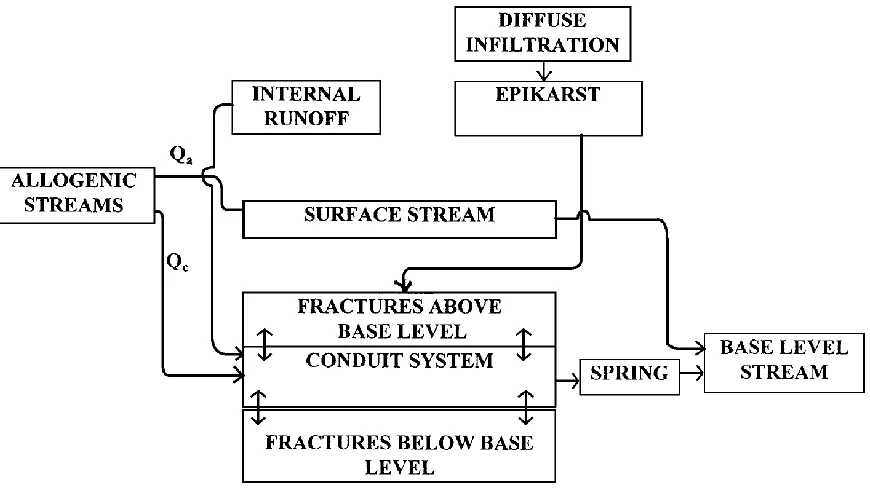
[image:37.612.106.541.416.660.2]The conceptual model of a karst aquifer can be drawn in various forms but the essential features remain the same. White (2002) provided the conceptual model shown below in Figure 2.2. The features of this model shall be discussed in the subsections that follow.
Table 2.1: Hydraulic classification of carbonate aquifers (White, 1969)
Flow Type Hydrological Control Associated Cave Type
Diffuse Flow Gross Lithology.
Shaley limestones; crystalline dolomites; high permeability porosity
Caves rare, small, have irregular patterns
Free Flow Thick, massive soluble rocks. Integrated conduit cave systems
Perched Karst system underlain by impervious rocks near or above base level
Cave streams perched – often have free air surface
Open Soluble rocks extend upward to level surface Sinkhole inputs: heavy sediment load; short
channel morphology caves
Capped Aquifer overlain by impervious rock Vertical shaft inputs; lateral flow under
capping beds; long integrated caves Deep Karst system extends to considerable depth below
base level
Flow is through submerged conduits
Open Soluble rocks extend to land surface Short tubular abandoned caves likely to be
sediment-choked
Capped Aquifer overlain by impervious rocks Long, integrated conduits under caprock.
Active level of system inundated
Confined Flow Structural and stratigraphic controls.
Artesian Impervious beds which force flow below regional base
level
Inclined 3-D network caves
Sandwich Thin beds of soluble rock between impervious beds Horizontal 2-D network caves.
2.2.1 Recharge
A characterisation of hydrology in karst lands is high infiltration and low surface runoff. For instance, in the Parnasos-Ghiona area in Greece, infiltration into the limestone aquifer has been calculated to be 45.2% while surface runoff is only 3.6% (Burdon and Papakis, 1961). This infiltration from rainfall can be divided into two components: allogenic recharge and autogenic recharge.
Autogenic recharge is the recharge that enters the aquifer directly from the overlying soil. It can be separated, as suggested by Gunn (1983), into two components: Diffuse Infiltration and Internal Runoff. Diffuse infiltration can be considered as comparable to any other hydrological setting. The initial precipitation is absorbed by the soil until the soil becomes saturated at which point the water percolates down through the matrix porosity or along fractures in the bedrock until it reaches the water table (Shaw, 2011). It should be noted however that in karst, the infiltration rate is much higher than in other hydrological settings due to the high permeability of rock and the fact that flow mainly crosses soil vertically rather than horizontally. Internal runoff is storm flow and is equivalent to overland flow in the usual hydrological cycle. Storm flow runoff flows into closed depressions (dolines) where the storm water enters the aquifer quickly through sinkhole drains (White, 2002).
Autogenic and allogenic recharge styles differ in terms of recharge per unit area and water chemistry with considerable consequences on the scale and distribution of the development of secondary permeability (Ford and Williams, 2007). The differences between autogenic and allogenic recharge are presented in Figure 2.3.
Figure 2.3: Illustration displaying duality of recharge (allogenic vs. autogenic) and infiltration (point vs. diffuse) (Goldscheider and Drew, 2007).
along fractures (‘grikes’ or ‘cutters’). Water can be forced to move laterally for considerable distances before being able to descend into the bedrock. Thus the epikarst provides a temporary storage with water requiring days or weeks to reach the groundwater system (Williams, 1983).
The volume of recharge entering the karst aquifer is regulated by the capacity of the input passages or catchment control (Palmer, 1984). If the inflow from surface streams is too great then the system will start to back up and ponding will occur, giving rise to surface streams or surface flooding. If the carrying capacity is not sufficient to carry even the minimum surface flow, this will result in a permanent surface stream. Localised flooding may also occur if the infiltration capacity of a swallow-hole is not sufficient due to a constriction or obstruction at the input point.
2.2.2
Flow Systems
Water in a karst aquifer moves down-gradient through the aquifer using a combination of three distinct types of porosity (triple permeability) models (White and White, 2005):
Matrix permeability: The intergranular permeability of the unfractured bedrock.
Fracture permeability: Mechanical joints, joint swarms and bedding plane partings, all of these possibly enlarged by solution.
Conduit permeability: Pipe-like openings with apertures ranging from 1 cm to a few tens of
meters.
These three elements of permeability carry different roles within the karst aquifer, with differing aperture sizes, distributions and flow mechanisms defined for each type. See Table 2.2 for a summary of their essential characteristics.
Table 2.2: Essential characteristics of triple permeability model (White and White, 2005)
Permeability Aperture Travel Time Flow Mechanism Distribution
Matrix µm to mm Long Darcian flow field. Laminar
Continuous medium
Fracture 10 µm to 10 mm Intermediate
Cube Law. Mostly laminar; may be non-linear components
Localised but statistically distributed
Conduit 10 mm to 10m Short
Darcy-Weisbach. Open channel and pipe flow. Turbulent.
MATRIX
Matrix flow through a karst aquifer is not fundamentally different from ground water flow in any other aquifer. The guiding equation is Darcy’s Law (Darcy, 1856). However the hydraulic conductivity of the rock (for use with Darcy’s law) is difficult to ascertain as the usual technique, pump tests on wells, is dominated by the fracture flow component (White and White, 2005). Though matrix porosity (2-11%) is shown to be much larger than the sum of fracture and conduit porosities (0.5 and 0.2%), its contribution to the hydraulic conductivity is practically negligible (Zuber and Motyka, 1998). As a result, matrix flow is often ignored. Matrix flow is assumed to follow in a lognormal distribution (Ford and Williams, 2007).
FRACTURES
The term ‘fracture’ (or ‘fissure’) is used to encompass single joints, joint swarms and bedding plane partings. Fracture apertures normally range between 50 - 500 µm. When fractures reach a width of 1cm, they are deemed as conduits (White, 2002). Under the assumptions of parallel walls and uniform aperture, fracture permeability can be modelled using the cubic law (derived from the Navier-Stokes equations) (White and White, 2005) which states that:
Equation 2.1
and,
Equation 2.2
where b is the full aperture of fracture, µ is the dynamic viscosity of water, w is the fracture width, dh/dl is the hydraulic gradient and K is the hydraulic conductivity. Fracture apertures are also assumed to follow a lognormal distribution.
CONDUITS
investigation. However spring hydrochemistry and tracer tests (as discussed in Section 2.4) can prove their presence. Conduits are typically elliptical in shape since corrosion is equal in all directions but concentrates along the guiding bedding planes (Ford and Williams, 2007).
Conduit flow in a single conduit with radius r in the laminar regime can be described by the Hagen-Poiseuille equation:
Equation 2.3
When the flow regime is turbulent, the Darcy-Weisbach equation can be used (assuming circular cross section). This gives:
( ) (
) Equation 2.4
However the use of this equation relies on a value for the Darcy-Weisbach friction factor, f, which must be determined empirically. It can be determined either by directly investigating the wall roughness of the conduit in question or can be back-calculated when all other parameters in the equation are known.
Friction factors have been calculated for numerous karst aquifers by different investigations such as Gale (1984), Atkinson et al. (1983) and Jeannin (2001) among others. The friction factors obtained cover a large range (0.039-340). Some studies such as Atkinson et al. (1983) and Lauritzen et al. (1985) calculated f by both approaches (investigation of conduit and back-calculation) and found that back-calculation tends to give dramatically higher results of f. However, as the friction factor is square rooted in the Darcy-Weisbach equation, the effect of different values is dampened. The study carried out by Lauritzen et al. (1985) was on an active phreatic conduit in Norway. The study found that the Darcy-Weisbach friction factor, f, decreases dramatically as discharge increases but levels out when discharge reaches 10 m3/s.
al., 2000b), Canada, England and Mexico (Ford and Williams, 2007) have found similar results with approximately 95% of storage within the rock matrix. It should be noted however that some aquifers have a relatively small phreatic zone compared to the epikarst and vadose zones. In these aquifers, the storage in the epikarst and vadose zones can be significant, possibly more than in the phreatic zone (Perrin et al., 2003)
2.2.3 Discharge
Groundwater from karst aquifers is usually discharged back to surface routes through large springs. In fact most of the largest springs in the world are from karst aquifers. They represent the end of underground river systems and mark the point at which surface processes become more dominant (Ford and Williams, 2007). The largest spring in the world is the Tobio spring in Papua New Guinea with a mean flow of between 85-115 m3/s (Maire, 1981). White (2002) categorised springs into 5 types:
i. Open conduit gravity springs where water emerges from an open cave mouth.
ii. Alluviated conduit springs where water emerges from a rise pool formed by a blockage of glacial or alluvial material.
iii. Rise pools discharging water from shallow flooded conduits. iv. Artesian springs where water rises from considerable depths.
v. Springs that discharge from solutionally widened fracture swarms.
There is great variety in the physical forms and rates of discharge from different springs. Sometimes spring clusters can form where the discharges from multiple drainage basins can have springs in the same general area. Over the last decade, useful information on spring discharge systems has been provided by cave divers particularly for spring types (iii) and (iv) (White, 2002).
The flow behaviour, turbidity and chemistry of springs are considered to strongly reflect the aquifer from which the spring is draining and, as a result, are extensively used as gauging points, sampling points and monitoring points for karst aquifers.
Figure 2.4: Estavelle at Coy Turlough. Acting as sink in summer (a) and a spring in winter (b)
2.2.4 Chemistry
The chemistry of the dissolution of calcite and dolomite reached an advanced formulation in the 1980s with the publication of reliable values for equilibrium constants (Plummer and Busenberg, 1982). This study identified the pertinent complexes and their role in the chemistry and established useful parameters such as hardness, saturation index and calculated carbon dioxide partial pressure. These chemical calculations can now be carried out using several speciation and reaction path computer programs such as WATEQ4F, MINTEQA2 and PHREEQE (available from the US Geological Survey and the US Environmental Protection Agency) (Langmuir, 1997).
The development of a karst aquifer is mostly a matter of the dissolution reactions rather than the final equilibrium state of these reactions. A paper by Plummer et al. (1978), was the first to attempt to classify the different chemical reactions. The individual rates of these reactions are summed to provide an overall dissolution rate for calcite. The reactions are set out below:
Equation 2.5
Equation 2.6
Equation 2.7
Each reaction is described for a forward reaction term in the rate equation:
Equation 2.8
This rate equation is known as the PWP equation (after Plummer, Wigley and Parkhurst (1978)). The first term is mass transfer-controlled but the second and third terms are reaction rate-controlled so that, in the pH range common to karst ground waters, the dissolution rate is only slightly dependent on flow regime.
Further investigations of reaction rates (Dreybrodt and Buhmann, 1991) have made use of a generic rate equation:
( ) Equation 2.9
where, A = area, V = volume of solution, k = reaction rate constant, C = concentration of dissolved carbonate, Cs = equilibrium saturation concentration for the dissolved carbonate and n = reaction order.
The reaction order can be determined empirically and shows that there is a break in the reaction rate at about 85% saturation (White, 2002). It was found that when the water is less than 85% saturated with CaCO3 the reaction is approximately first order causing rapid dissolution but approaches a slower fourth order reaction rate as saturation reaches 85% (Svensson and Dreybrodt, 1992). This break is very significant in the development of conduit permeability as it stops the water from becoming overly saturated which would prevent further conduit development.
Further investigations (Liu and Dreybrodt, 1997, Svensson and Dreybrodt, 1992) of dissolution kinetics under turbulent flow and near equilibrium conditions have revealed additional controls.
The hydration reaction of aqueous CO2 to H2CO3 is shown to be rate-controlling when the
A/V ratios are high and under some conditions of turbulent flow.
Adsorption of ions on the reactive surface becomes rate-controlling under near-saturation
conditions.
2.3
Karst Network Development
Significant changes to a karst aquifer in terms of flow paths and conduit network can take place over thousands of years which, on a geologic timescale, makes it a very rapid process. The fractures are solutionally enlarged by flow under laminar flow conditions into conduits where turbulent flow conditions prevail (Ford and Williams, 2007).
2.3.1 Energy Supply
The development of a flow network in a carbonate aquifer depends on the energy supply available and its spatial distribution. Ford and Williams (2007) describe how this is mainly from:
i. The throughput volume of water.
ii. The difference in elevation between the recharge and discharge areas (i.e. hydraulic gradient).
iii. The spatial distribution of recharge, i.e. on whether it is evenly distributed (autogenic recharge) or is focused (allogenic point recharge).
iv. The chemical aggressivity of the recharging waters.
If the aquifer is close to a volcanic or hot spring region, the geothermal heat flux may also be important. Dissolution is a key factor in the development of a karst aquifer (and is directly related to the amount of rainfall) but in addition to this chemical energy, the primary forms of fluid energy are potential, kinetic and internal energy.
Most of the potential energy is realised as kinetic energy as water descends down through the vadose zone where a large amount of mechanical work can be done by fluvial processes.
pulse travels down the cave passage as a kinematic wave until the saturated zone is reached and a pressure pulse is forced through the phreatic conduits giving a hydrograph peak at the spring. This is known as piston flow (Ford and Williams, 2007).
Internal energy, best represented by rock and water temperature, is another significant form of energy in an aquifer. Temperature is important because of the effect it has on the dynamic (and kinematic) viscosity of water which is more than twice as viscous at 0°C as at 30°C. Thus the lower viscosity at higher temperatures allows greater discharge through capillary tubes (Poiseuille’s law) and increases hydraulic conductivity. This influence of temperature is therefore a good explanation for the differences between karst in cool temperate and more tropical zones.
2.3.2 Fracture Enlargement
Carbonate aquifers are not the only type to experience fracture flow. For example, there are fractured quartzites, granites and basalts, all of which can be effective aquifers. The difference between these types and carbonate aquifers is that, in carbonate aquifers, the fractures enlarge much quicker with time and ground water circulation. Once water has entered the aquifer, the various forms of energy mentioned above are used up in the enlargement of primary pores and fractures into secondary conduit networks. White (2002) has described how, in the early stages of this process, there are three thresholds that appear when the aperture exceeds about 0.01m, these are: hydraulic, kinetic and transport.
HYDRAULIC THRESHOLD
The hydraulic threshold permits the breakdown of laminar flow and the onset of turbulent flow. In principle it is quite straightforward. Flow in the fractures will be laminar and follows Darcy’s Law until the Reynolds number reaches the range of approximately 500 and turbulent flow starts to take over.
KINETIC THRESHOLD
laminar flow penetrates deep into the aquifer. This water continues to slowly dissolve its way through the aquifer until ‘break-through’ occurs. This is the point at which an aperture/pathway has enlarged enough to allow water with less than 85% saturation to penetrate the entire aquifer. When this occurs, the kinetics shift from fourth order back to first order and the rate of dissolution dramatically increases causing a runaway process which allows the chosen pathway to enlarge rapidly. This threshold explains why the number of fully developed conduits is usually much smaller than the number of fractures.
TRANSPORT THRESHOLD
The transport threshold enables flow velocities to be sufficient for the transport of clastic material. These particles can range in size from colloids to boulders either as bed load or suspended load. Transport of these particles is not completely understood but it is known that the critical velocities for sediment movement are very similar to the velocities at the onset of turbulence. Thus the transport threshold occurs at near the same aperture as the other thresholds.
The coincidence of these three thresholds at 0.01m provides a natural division between fractures and conduits as well as separating the process of conduit development into an initiation phase where fractures grow to critical threshold and an enlargement phase as the conduit then expands to the size of a typical cave passage.
2.3.3 Development of Vadose Zone and Epikarst
Unkarstified crystalline carbonate rocks typically have very low primary porosity (≈2%). Thus when fresh water first meets the rock, the standing water level in the rock is close to the surface. Porosity and permeability of the karst increases over time and consequently more void space becomes available to store and transmit groundwater. As a result, the water level gradually falls and so the aerated zone becomes deeper. As this is happening the surface level also drops due to denudation which means the resultant thickness of the vadose zone depends on its upper (surface) and lower (water table) boundaries. The vadose zone in well-karstified rock can extend to as much as 2 km below the surface (Ford and Williams, 2007).
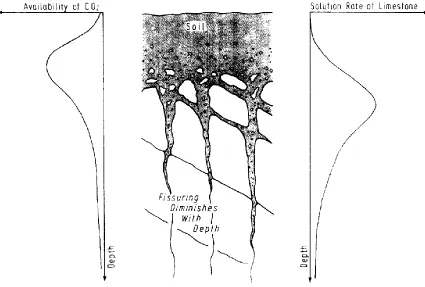
erosion. With percolation water available, solution is greatest near the surface because of the relative abundance of carbon dioxide and thus carbonic acid in the soil. As the water percolates downwards, there is less CO2 available to the solution and thus the capacity for continued corrosion is diminished as the solution approaches equilibrium. This is illustrated in Figure 2.5. The amount and depth of solution varies with rainfall, time, lithology, soil composition, soil thickness, the partial pressure of CO2 and the nature of the solution system (i.e. ‘open’ or ‘closed’).
Figure 2.5: Relationship between soil CO2, rate of limestone solution and fissuring beneath the
soil. (Williams, 1983)
percolation into cave systems over dry periods. These aquifers are also used as water supplies with many epikarstic springs being used to supply local water-schemes, especially in China (Williams, 2008). An excellent example of epikarst is the Burren in County Clare as the bare, crystalline, carboniferous hills have been stripped of protective cover during the Pleistocene to reveal a glacially-polished limestone surface containing solutionally enlarged fissures (or ‘grikes’).
Unlike the majority of karst aquifers found around the globe, the karst aquifers found in Ireland (such as in the catchment under study in this thesis) are predominantly lowland regions. As such, the vadose zone in Irish karsts can be relatively shallow which often results in epikarst occurring within the phreatic or epiphreatic zone. Due to this, a significant quantity of diffuse flow through an Irish karstic aquifer can be flowing through the epikarstic zone, i.e. horizontal flow occurring within epikarst rather than (the more typical) vertical flow.
2.3.4 Conduit Network Development
INITIATION
The main concept for the initiation of conduit permeability is that of an initial pathway connecting the recharge area to the (future) drainage area by means of joints, joint swarms and bedding plane partings. Water is driven through the sequence of fractures due to the head difference between inlet and outlet. As mentioned above, the apertures increase slowly under fourth order kinetics until they become wide enough to allow the total penetration of under-saturated water from entry to exit. After the relatively short time of 5000-10,000 years, turbulent flow may be first encountered. This is known as ‘breakthrough’ (Dreybrodt, 1990). Groves and Howard (1994b) concluded that, due to the sensitivity of breakthrough time to the initial aperture, breakthrough would not occur in apertures below a few hundred micrometres and thus, conduits would not form.
With models constructed for single fractures, the next step is to extend the calculations to multiple fractures which make up a flow path in an aquifer. Groves and Howard (1994a) developed a model which started on a hypothetical grid of fractures at very wide spacings. Siemers and Dreybrodt (1998) then developed a model with smaller fracture spacing which introduced a probability that any given fracture segment on the grid could be connected to other fractures and thus could contribute to the flow path. Many of these modelling attempts assume a simple geometry of plane parallel fractures, fixed apertures and uniform cross-section. As a result, the flow through the fracture is proportional to the cube of the aperture. However, in reality a correction to the cube law is required as fractures have rough walls, and variable aperture sizes (Oron and Berkowitz, 1998). These models validate what is seen in nature that karst networks developing very few large conduit channels with diffuse flow through numerous small fractures.
CONDUIT ENLARGEMENT AND INTEGRATION
When the optimum flow path has been determined and the aperture size has reached the value of approximately 0.01m, the under-saturated water now traverses the entire width of the aquifer and the dissolution kinetics shift into a more or less linear regime. Palmer (1991), showed that the rate of retreat of conduit wall depended only on the degree of saturation and is described by equation 2.10:
( ) Equation 2.10
where S = rate of wall retreat (cm/yr), k1 = 1st order reaction rate constant, C = concentration of dissolved carbonate, Cs = saturation concentration of dissolved carbonate, n = reaction order and ρR = density of bedrock.
Values of k1 and n have been determined experimentally by Palmer (1991). It has been found that the maximum rate of wall retreat is from 0.01 to 0.1 cm/yr. At this dissolution rate, an active conduit can enlarge from a threshold conduit (0.01m) to the diameter of a meter within a few thousand years.