Time Preference Shocks

Munich Personal RePEc Archive

Time Preference Shocks

Harashima, Taiji

Kanazawa Seiryo University

26 November 2014

Online at

https://mpra.ub.uni-muenchen.de/60205/

Time Preference Shocks

Taiji Harashima

*

Abstract

The rate of time preference (RTP) has traditionally not been regarded as an important source of economic fluctuations. In this paper, I show that it is an important factor influencing economic fluctuations because households must have an expected RTP for the representative household (RTP RH) to behave optimally. Because it is impossible for a household to know the intrinsic RTP RH, it cannot know the parameters of the structural model of the RTP RH. Without a structural model, a household must use its beliefs to generate an expected RTP RH. As a result, the expected value can change more frequently than the intrinsic RTP RH. Because households often change their beliefs about their expected future paths, economic fluctuations caused by time preference shocks also can occur more frequently in an economy than previously thought.

JEL Classification code: D90, E13, E32

Keywords: Time preference; Economic fluctuations; Business cycles; The representative household; Sustainable heterogeneity

*Correspondence: Taiji HARASHIMA, Kanazawa Seiryo University, 10-1 Goshomachi-Ushi, Kanazawa-shi, Ishikawa, 920-8620, Japan.

INTRODUCTION

The rate of time preference (RTP) plays an essential role in economic activities, and its importance has been emphasized since the era of Irving Fisher (Fisher, 1930). One of the most important equations in economics is the steady state condition

r

θ , (1)

where θ is RTP and r is the real rate of interest. This condition is a foundation of both static and dynamic economic studies. In this sense, the mechanisms of both θ and r are equally important. Although the mechanism of r (i.e., how r is determined) has been widely studied, RTP has not necessarily been regarded as an essential subject of economic research. For example, only factors that affect r (e.g., technology shocks or monetary shocks) have been studied as a source of economic fluctuations. RTP has been generally neglected because it has been widely believed that RTP is merely an intrinsically constant parameter. Some have argued that RTP is changeable even over short periods (e.g., Uzawa, 1968; Epstein and Hynes, 1983; Lucas and Stokey, 1984; Parkin, 1988; Obstfeld, 1990; Becker and Mulligan, 1997), but little attention has been given to these discussions. If RTP is truly constant and given exogenously, there may be little room for further meaningful research on the topic because shocks on RTP would not exist and would therefore not be an important source of economic fluctuations. Conversely, if RTP is not constant and is able to change frequently, current economic theories may have to be substantially rethought. In this case, RTP would have to be examined as an important source of economic fluctuations because the RTP, as the discount factor for future utility, is an essential element in economic activities.

In dynamic macroeconomic models, the RTP of the representative household (hereafter, RTP RH) matters. It has usually been assumed to be a constant parameter representing the RTPs of all households, usually the average RTP of all households. However, as Becker (1980) and Harashima (2014) showed, this assumption is impossible in dynamic models unless the RTPs of all households are also assumed to be identical. Otherwise, there is no state where all optimality conditions of all households are satisfied. The assumption of identical RTPs is problematic because this assumption is not merely expedient for the sake of simplicity; rather, it is a critical requirement that allows for an assumed representative household. Therefore, the rationale for the assumption of identical RTPs should be validated because it is unquestionably not identical among households. Hence, the indispensable nature of the assumption of identical RTPs leads to questions about the validity of studies based on dynamic models that define the representative household as the average household.

In this paper, I present an alternative definition of the representative household that can be used in dynamic models (see Harashima, 2014). This new definition, however, leads to the important requirement that each household must ex ante know the RTP RH to achieve optimality. The traditional definition (i.e., the representative household as the average household) allows the assumption that each household behaves without considering other households’ optimality. That is, there is no need to ex ante know the RTP of the representative household as well as the RTPs of other households, assuming that the ex post aggregates are consistent with the representative household’s behavior and the RTP RH. In contrast, the alternative definition necessitates that all households must ex ante know the RTP RH for them to optimize their behavior. Otherwise, the ex post aggregates cannot be consistent with the

representative household’s behavior. Hence, each household must ex ante generate an expected RTP RH to optimize its objectives.

Several endogenous RTP models have been presented, the most well-known of which is that of

Uzawa (1968). However, Uzawa’s model has not necessarily been regarded as a realistic

expression of RTP endogeneity because it has a serious drawback in that impatience increases as income, consumption, and utility increase. In this paper, an alternative structural model of RTP is presented that does not suffer from this drawback.

There is another critical obstacle. Although a household knows its own RTP, it has almost no information about RTPs of all of the other households or of the RTP RH. Hence, a household must use its beliefs about the RTP RH to form its expected RTP RH. Households may behave based on bounded rationality and use heuristics in this type of situation. As a result, even if the intrinsic RTP RH does not change, the expected RTP RH can change if the household’s belief changes. Therefore, it is likely that households’ expected RTP change more frequently than the intrinsic RTP RH, i.e., time preference shocks occur more frequently than has been previously thought.

The paper is organized as follows. Section 2 shows that the representative household defined as the average household is impossible to use in dynamic models, and an alternative definition is presented. Section 3 shows that the necessity of households having an expected RTP RH to achieve optimality is also discussed. In Section 4, a structural model of RTP is developed. In Section 5, I show that the structural model cannot be used because households cannot know the intrinsic RTP RH, and that households must generate an expected RTP RH based on beliefs. Therefore, time preference shocks occur more frequently than has been traditionally thought. Finally, I offer concluding remarks in Section 6.

2 THE REPRESENTATIVE HOUSEHOLD

2.1 The representative household in dynamic models

2.1.1 The assumption of the representative household

The concept of the representative household is a necessity in macroeconomic studies. It is used as a matter of course, but its theoretical foundation is fragile. The representative household has been used given the assumption that all households are identical or that there exists one specific individual household, the actions of which are always average among households (I call such a household “the average household” in this paper). The assumption that all households are identical seems to be too strict; therefore, it is usually assumed explicitly or implicitly that the representative household is the average household. However, the average household can exist only under very strict conditions. Antonelli (1886) showed that the existence of an average household requires that all households have homothetic and homogeneous utility functions. This type of utility function is not usually assumed in macroeconomic studies because it is very restrictive and unrealistic. If more general utility functions are assumed, however, the assumption of the representative household as the average household is inconsistent with the assumptions underlying the utility functions.

Nevertheless, the assumption of the representative household has been widely used, probably because it has been believed that the representative household can be interpreted as an approximation of the average household. Particularly in static models, the representative household can be seen to approximate the average household. However, in dynamic models, it is hard to accept the representative household as an approximation of the average household because, if RTPs of households are heterogeneous, there is no steady state where all of the optimality conditions of the heterogeneous households are satisfied (Becker, 1980). Therefore, macroeconomic studies using dynamic models are fallacious if the representative household is assumed to approximate the average household.

Static models are usually used to analyze comparative statics. If the average household is represented by one specific unique household for any static state, there will be no problem in assuming the representative household as an approximation of the average household. Even though the average household is not always represented by one specific unique household in some states, if the average household is always represented by a household in a set of households that are very similar in preferences and other features, then the representative household assumption can be used to approximate the average household.

Suppose, for simplicity, that households are heterogeneous such that they are identical except for a particular preference. Because of the heterogeneous preference, household consumption varies. However, levels of consumption will not be distributed randomly because the distribution of consumption will correspond to the distribution of the preference. The consumption of a household that has a very different preference from the average will be very different from the average household consumption. Conversely, it is likely that the consumption of a household that has the average preference will nearly have the average consumption. In addition, the order of the degree of consumption will be almost unchanged for any static state because the order of the degree of the preference does not change for the given state.

If the order of consumption is unchanged for any given static state, it is likely that the household with consumption that is closest to the average consumption will also always be a household belonging to a group of households that have very similar preferences. Hence, it is possible to argue that, approximately, one specific unique household’s consumption is always average for any static state. Of course, it is possible to show evidence that is counter to this argument, particularly in some special situations, but it is likely that this conjecture is usually true in normal situations, and the assumption that the representative household approximates the average household is acceptable in static models.

2.1.3 The representative household in dynamic models

In dynamic models, however, the story is more complicated. In particular, heterogeneous RTPs pose a serious problem. This problem is easily understood in a dynamic model with exogenous technology (i.e., a Ramsey growth model). Suppose that households are heterogeneous in RTP, degree of risk aversion (ε), and productivity of the labor they provide. Suppose also for simplicity that there are many “economies” in a country, and an economy consists of a household and a firm. The household provides labor to the firm in the particular economy, and the firm’s level of technology (A) varies depending on the productivity of labor that the household in its economy provides. Economies trade with each other: that is, the entire economy of a country consists of many individual small economies that trade with each other.

A household maximizes its expected utility, E



u

 

c_t exp



θt



dt 0

, subject to

 

t t t f k c

k   , where u

 

 is the utility function; f

 

 is the production function; θ is RTP; E is the expectation operator;

t t t

L Y

y  ,

t t t

L K

k  , and

t t t

L C

c  ; Yt (≥ 0) is output, Kt (≥ 0)

is capital input, Lt (≥ 0) is labor input, and Ct (≥ 0) is consumption in period t. The optimal

consumption path of this Ramsey-type growth model is

   

 

     _θ

k y

ε

c c

t t t

t 1 

,

and at steady state,

θ

k y

t t   

Therefore, at steady state, the heterogeneity in the degree of risk aversion (ε) is irrelevant, and the heterogeneity in productivity does not result in permanent trade imbalances among

economies because

t t

k y

 

in all economies is kept equal by market arbitrage. Hence,

heterogeneity in the degree of risk aversion and productivity does not matter at steady state. Therefore, the same logic as that used for static models can be applied. Approximately, one specific unique household’s consumption is always average for any time in dynamic models, even if the degree of risk aversion and the productivity are heterogeneous. Thus, the assumption of the representative household is also acceptable in dynamic models even if the degree of risk aversion and the productivity are heterogeneous.

However, equation (2) clearly indicates that heterogeneity in RTP is problematic. As Becker (1980) shows, if RTP is heterogeneous, the household that has the lowest RTP will eventually possess all capital. With heterogeneous RTPs, there is no steady state where all households achieve all of their optimality conditions. In addition, the household with consumption that is average at present has a very different RTP from the household with consumption that is average in the distant future. The consumption of a household that has the average RTP will initially be almost average, but in the future the household with the lowest RTP will be the one with consumption that is almost average. That is, the consumption path of the household that presently has average consumption is notably different from that of the household with average consumption in the future. Therefore, any individual household cannot be almost average in any period and thus cannot even approximate the average household. As a result, even if the representative household is assumed in a dynamic model, its discounted expected utility E



u

 

c_t exp



θt



dt

0 is meaningless, and analyses based on it are

fallacious.

If we assume that RTP is identical for all households, the above problem is solved. However, this solution is still problematic because that assumption is not merely expedient for the sake of simplicity; rather, it is a critical requirement to allow for an assumed representative household. Therefore, the rationale for identical RTPs should be validated; that is, it should be demonstrated that identical RTPs are actually and universally observed. RTP is, however, unquestionably not identical among households. Hence, it is difficult to accept the representative household assumption in dynamic models based on the assumption of identical RTP.

The conclusion that the representative household assumption in dynamic models is meaningless and leads to fallacious results is very important, because a huge number of studies have used the representative household assumption in dynamic models. To solve this severe problem, an alternative interpretation or definition of the representative household is needed.

Note that in an endogenous growth model the situation is even more complicated. Because a heterogeneous degree of risk aversion also matters, the assumption of the representative household is more difficult to accept, so an alternative interpretation or definition is even more important when endogenous growth models are used.

2.2 Sustainable heterogeneity

2.2.1 The model

Suppose that two heterogeneous economies―economy 1 and economy 2—are identical except

for their RTPs. Households within each economy are assumed to be identical for simplicity. The population growth rate is zero. The economies are fully open to each other, and goods, services, and capital are freely transacted between them, but labor is immobilized in each economy.

Because the economies are fully open, they are integrated through trade and form a combined economy. The combined economy is the world economy in the international interpretation and the national economy in the national interpretation. In the following discussion, a model based on the international interpretation is called an international model and that based on the national interpretation is called a national model. Usually, the concept of the balance of payments is used only for the international transactions. However, because both national and international interpretations are possible, this concept and terminology are also used for the national models in this paper.

RTP of household in economy 1 is θ₁ and that in economy 2 is θ2, and θ1 < θ2. The

production function in economy 1 is y_1,t  Aαf

 

k_1,t and that in economy 2 is

 

,t

α

,t A f k

y₂  ₂ , where yi,t and ki,t are, respectively, output and capital per capita in economy i

in period t for i = 1, 2; A is technology; and α



0α1



is a constant. The population of each economy is

2

L_{; thus, the total for both is L, which is sufficiently large. Firms operate in both}

economies. The current account balance in economy 1 is τt and that in economy 2 is –τt. The

production functions are specified as

α

t i,

α

i,t A k

y  1 _;

thus, 1

  

1,2



,

,  

 _{AL i}

K

Y_{it it}α α . Because A is given exogenously, this model is an exogenous technology model (Ramsey growth model). The examination of sustainable heterogeneity based on an endogenous growth model is shown in Appendix.

Because both economies are fully open, returns on investments in each economy are kept equal through arbitration, such that

,t ,t ,t ,t k y k y 2 2 1 1     

. (3)

Because equation (3) always holds through arbitration, equations k1,_t k2,_t , k1,t k2,t ,

t t y

y1,  2, , and y1,t  y2,t also hold.

The accumulated current account balance



₀tτsds mirrors capital flows between the two

economies. The economy with current account surpluses invests them in the other economy.

Because _

           t t t t k y k y , 2 , 2 , 1 ,

1 _{are returns on investments,}

ds τ k y t s t t



  0 , 1 ,

1 _and

ds τ k y t s t t



  0 , 2 , 2

represent income receipts or payments on the assets that an economy owns in the other economy. Hence,

ds

τ

k y

τ t s

t t t _



  0 , 2 , 2

is the balance on goods and services of economy 1, and

is that of economy 2. Because the current account balance mirrors capital flows between the economies, the balance is a function of capital in both economies, such that



,t ,t



t κ k ,k

τ  1 2 .

The government (or an international supranational organization) intervenes in the activities of economies 1 and 2 by transferring money from economy 1 to economy 2. The amount of transfer in period t is gt, and it is assumed that gt depends on capital inputs, such that

,t t gk

g  _{1 ,}

where g is a constant. Because k_1,t k_2,t and k_1,t k_2,t,

,t ,t

t gk gk

g  ₁  ₂ .

Each household in economy 1 therefore maximizes its expected utility

 

c



θ t



dt u

E



₀ 1 1,t exp  1



,

subject to





t ,t

t s α ,t α ,t α ,t α

t A k c α A k τ ds τ gk

k ₁ 0 1 1 1 1 ,

1    1



 

 

 _{, (4)}

and each household in economy 2 maximizes its expected utility

 

c



θ t



dt u

E _{t 2}

0 2 2, exp 



 ,

subject to





t t

t s α t α ,t α t α

t A k c α A k τ ds τ gk

k _2,

0 , 2 2 1 , 2 ,

2    1



 

 

 _{, (5)}

where ui,t and ci,t, respectively, are the utility function and per capita consumption in economy i

in period t for i = 1, 2; and E is the expectation operator. Equations (4) and (5) implicitly assume that each economy does not have foreign assets or debt in period t = 0.

2.2.2 Sustainable heterogeneity

without government intervention

Heterogeneity is defined as being sustainable if all of the optimality conditions of all heterogeneous households are satisfied indefinitely. First, the natures of the model when the government does not intervene (i.e., g0) are examined. The growth rate of consumption in economy 1 is



1





1





1



0 lim lim ₁ 1 0 1 , 1 1 0 , 1 , 1 1 , 1 , 1 _                        



 



   

 _k θ

τ ds τ k A α α k ds τ k A α k A α ε c c ,t t t s α t α ,t t s α t α α t α t t t t  and thereby



1





1



1





0

lim  ₁     ₁



 α Ak α Ψ Ξ θ

α ,t α t , where t t t t t t _k τ k τ Ξ , 2 , 1 lim lim     

 and

,t t s t ,t t s t _k ds τ k ds τ Ψ 2 0 1 0 lim

lim





      .       t t t t t t _c c y y , 1 , 1 , 1 , 1 lim

lim  

0 lim

lim

1

1 _{ }

    t t t ,t ,t t τ τ k

k 

, and Ψ is constant at steady state because k1,t and τt are constant; thus,

t t t _k τ Ξ , 1 lim  

 is constant at steady state. For Ψ to be constant at steady state, it is necessary that

0

lim 

  t

t τ

and thus Ξ0. Therefore,



1





1



1





0

lim  ₁    ₁



 α A k α Ψ θ α

,t

α

t

, (6)

and



1





1



1





0

lim  ₂    ₂ 



 α A k α Ψ θ

α ,t α t (7) because



1





1





1



0

lim lim 2 2 0 1 , 2 2 0 , 2 , 2 1 , 2 , 2                         



 

_

   

 _k θ

τ ds τ k A α α k ds τ k A α k A α ε c c ,t t t s α t α ,t t s α t α α t α t t t t  .

Because lim



1 α



A k₁,tα



1



1 α



Ψ



θ₁

α

t    

 

 , lim



1 α



A k2



1



1 α



Ψ



θ2 α

,t

α

t    

 

 ,

and α _,tα α _,tα

t t t t k A k A k y k

y _{ }

       2 1 . 2 , 2 . 1 ,

1 _{, then}





t t t _k y α θ θ Ψ . 1 , 1 2 1 lim 1 2       

. (8)

By equations (6) and (8),





1

1 1 1 1 1 lim

lim α Ψ θ

k y k y .t ,t t .t ,t

t   

.t ,t t .t ,t t _k y θ θ k y 2 2 2 1 1 1 _lim 2 lim          

 . (9)

If equation (9) holds, all of the optimality conditions of both economies are indefinitely satisfied. The state indicated by equation (9) is called the “multilateral steady state” or “multilateral state” in the following discussion. By procedures similar to those used for the endogenous growth model in Appendix, the condition of the multilateral steady state for H economies that are identical except for their RTPs is shown as

H θ k y H q q i.t i,t t



      1

lim (10)

for any i, where i = 1, 2, … , H. Because







1





0

lim 1

2 1 2

2 1 . 1 , 1 2 1             θ θ α θ θ k y α θ θ Ψ t t t

by equation (9), then by lim 0

1

0 _{ }





 _k Ψ

ds τ ,t t s t , 0 lim 0 



  τds

t s t

;

that is, economy 1 possesses accumulated debts owed to economy 2 at steady state, and economy 1 has to export goods and services to economy 2 by



α



Aαk_tα



tτ_sds 0 , 1

1

in every period to pay the debts. Nevertheless, because lim 0

  t

t τ and Ξ0, the debts do

not explode but stabilize at steady state. Because of the debts, the consumption of economy 1 is smaller than that of economy 2 at steady state under the condition of sustainable heterogeneity. Note that many empirical studies conclude that RTP is negatively correlated with income (e.g., Lawrance, 1991; Samwick, 1998; Ventura, 2003). Suppose that, in addition to the heterogeneity in RTP (θ1 < θ2), the productivity of economy 1 is higher than that of economy 2.

At steady state, the consumption of economy 1 would be larger than that of economy 2 as a result of the heterogeneity in productivity. However, as a result of the heterogeneity in RTP, the consumption of economy 1 is smaller than that of economy 2 at steady state under sustainable heterogeneity. Which effect prevails will depend on differences in the degrees of heterogeneity. For example, if the difference in productivity is relatively large whereas that in RTP is relatively small, the effect of the productivity difference will prevail and the consumption of economy 1 will be larger than that of economy 2 at steady state under sustainable heterogeneity.

2.2.3 Sustainable heterogeneity with government intervention

difference emerges because, in a multilateral state, economy 1 behaves by fully considering

economy 2’s conditions. The multilateral state therefore will not be naturally selected by economy 1, and the path selection may have to be decided politically (see Harashima, 2010). On the other hand, when economy 1 behaves unilaterally, the government may intervene in economic activities so as to achieve, for example, social justice.

In this section, I show that, even if economy 1 behaves unilaterally, sustainable heterogeneity can always be achieved with appropriate government intervention.

2.2.3.1 The two-economy model

Government intervention is first considered in the two-economy model constructed in Section 2.2.1. If the government intervenes (i.e., g0),





              t s t s t t t t t t t ds dt ds d c c 0 0 , 1 , 1 lim lim lim      .

Because g0, equations (6) and (7) are changed to



1





1



1





0

lim  1    1 

 

 α A k α Ψ θ g α

,t

α

t

, (11)

and



1





1



1





0

lim  ₂    ₂ 



 α A k α Ψ θ g α

,t

α

t

. (12)

If economy 1 behaves unilaterally such that equation (11) is satisfied, then

0 lim , 1 , 1    t t t _c c and



 







α k A α g θ Ψ α ,t α t          1 1 1

lim ₁ 1

1

.

At the same time, if economy 2 behaves unilaterally such that equation (12) is satisfied, then

0 lim , 2 , 2 _   t t t _c c .

By equations (11) and (12)



α



A k



α



Ψ θ

θ

g α _,tα

t  

 

 



 1 1

lim

2 1

1 2





.t ,t t .t ,t t α ,t α t _k y k y θ θ k A α 2 2 1 1 2 1

1 lim lim

2 1 lim                 .

This equation is identical to equation (9) and is satisfied at the multilateral steady state. Therefore,









,t t s t .t ,t t _k ds τ θ θ α θ θ Ψ k y α θ θ g 1 0 2 1 1 2 1 1 1 2 _lim 2 1 2 lim 1 2



             

 . (13)

If g is set equal to equation (13), all optimality conditions of both economies 1 and 2 are satisfied even though economy 1 behaves unilaterally.

There are various values of Ψ, depending on the initial consumption economy 1 sets. If

economy 1 behaves in such a way as to make lim 0

0 



  τ ds

t s t

, and particularly, make g= 0

such that





lim 0

2 1 2 1 0 2 1 1

2    





  ,t t s t _k ds τ θ θ α θ θ

g ,

then





t t t _k y α θ θ Ψ . 1 , 1 2 1 lim 1 2        (14)

by equation (13). Equation (14) is identical to equation (8); that is, the state where equation (14) is satisfied is identical to the multilateral state with no government intervention (i.e., g= 0).

On the other hand, if economy 1 behaves in such a way as to make lim 0

0 



  τ ds

t s t , 0 2 1 2 

θ θ

g .

This condition is identical to that for sustainable heterogeneity with government intervention in the endogenous growth model shown by Harashima (2012). Furthermore, if economy 1 behaves

in such a way as to make lim 0

0 



  τ ds

t s t

, g is positive and is given by equation (13).

There are various steady states, depending on the values of

,t t s t _k ds τ Ψ 1 0 lim



 

 and the

2.2.3.2 The multi-economy model

In this section, for simplicity, only the case of lim 0

1

0 _





 

,t t

s t _k

ds

τ

Ψ is considered. It is

assumed that there are H economies that are identical except for their RTPs. If H = 2, when sustainable heterogeneity is achieved, economies 1 and 2 consist of a combined economy

(economy 1+2) with twice the population and a RTP of

2 2 1 θ

θ 

. Suppose there is a third

economy with a RTP of θ3. Because economy 1+2 has twice the population of economy 3, if

3 2

2 1 3

θ θ θ g

 

 ,

then

0 lim

lim lim

, 3

, 3

, 2

, 2

, 1

,

1 _{  }

  

 



t t t t t t t t

t _c

c

c c

c

c  

.

By iterating similar procedures, if government transfer between economy H and economy 1+2+

∙ ∙ ∙ + (H– 1) is such that

H H

θ θ

g

H

q q H

1

1

1

  







,

then

0 lim

, , _

 

t i

t i t _c

c

for any i(= 1, 2, ∙ ∙ ∙, H).

2.3 An alternative definition of the representative household

2.3.1 The definition

Section 2.2 indicates that, when sustainable heterogeneity is achieved, all heterogeneous households are connected (in the sense that all households behave by considering other households’ optimality) and appear to be behaving collectively as a combined supra-household that unites all households, as equations (9) and (10) indicate. The supra-household is unique and its behavior is time-consistent. Its actions always and consistently represent those of all households. Considering these natures of households under sustainable heterogeneity, I present the following alternative definition of the representative household: “the behavior of the representative household is defined as the collective behavior of all households under sustainable heterogeneity.”

household has a RTP that is equal to the average RTP as shown in equations (9) and (10).1 Hence, we can assume not only a representative household but also that its RTP is the average rate of all households.

2.3.2 Universality of sustainable heterogeneity

An important point, however, is that this alternatively defined representative household can be used in dynamic models only if sustainable heterogeneity is achieved, but this condition is not necessarily always naturally satisfied. Sustainable heterogeneity is achieved only if households with lower RTPs behave multilaterally or the government appropriately intervenes. Therefore, the representative household assumption is not necessarily naturally acceptable in dynamic models unless it is confirmed that sustainable heterogeneity is usually achieved in an economy. Notwithstanding this flaw, the representative household assumption has been widely used in many macroeconomic studies that use dynamic models. Furthermore, these studies have been little criticized for using the inappropriate representative household assumption. In addition, in most economies, the dire state that Becker (1980) predicts has not been observed even though RTPs of households are unquestionably heterogeneous. These facts conversely indicate that sustainable heterogeneity―probably with government interventions―has been usually and universally achieved across economies and time periods. In a sense, these facts are indirect evidence that sustainable heterogeneity usually prevails in economies.

Note that because the representative household’s behavior in dynamic models is represented by the collective behavior of all households under sustainable heterogeneity, RH’s RTP is not intrinsically known to households, but they do need to have an expected rate. Each household intrinsically knows its own preferences, but it does not intrinsically know the collective preference of all households. Therefore, in dynamic models, it must be assumed that all households do not ex ante know RH’s RTP, but households estimate it from information on the behaviors of other households and the government.

3 NEED FOR AN EXPECTED RTP RH

3.1 The behavior of household

Achieving sustainable heterogeneity affects the behavior of the individual household because sustainable heterogeneity indicates that each household must consider the other households’ optimality (as well as the behavior of the government, if necessary). This feature does not mean that households behave cooperatively with other households. Each household behaves non-cooperatively based on its own RTP, but at the same time, it behaves considering whether

the other households’ optimality conditions are achieved or not. This consideration affects the actions a household takes in that it affects the choice of a household’s initial consumption.

Sustainable heterogeneity indicates that a household’s future path of consumption has to be consistent with the future path of sustainable heterogeneity. Thereby, a household sets its initial consumption such that it will proceed on the path that is consistent with the path of sustainable heterogeneity and eventually reach a steady state.

3.2 Deviation from sustainable heterogeneity

3.2.1 Political elements

What happens if a household deviates from sustainable heterogeneity? A deviation means that a household sets its initial consumption at a level that is not consistent with sustainable heterogeneity. For less advantaged households (i.e., households with higher RTPs), the only way to satisfy all of their optimality conditions is to set their initial consumption consistent with

1

sustainable heterogeneity. Therefore, they will not take the initiative to deviate. In contrast, the most advantaged households (i.e., those with the lowest RTP) can satisfy all of their optimality conditions even if they set initial consumption independent of sustainable heterogeneity. The incentive for the most advantaged household to select a multilateral path will be weak because the growth rate of the most advantaged household on the multilateral path is lower than that on the unilateral path.

When economy 1 selects the unilateral path, does economy 2 quietly accept the unfavorable consequences shown in Becker (1980)? From an economic perspective, the optimal response of economy 2 is the one shown in Harashima (2010): economy 2 should behave as a follower and accept the unfavorable consequences. However, if other factors—particularly political ones—are taken into account, the response of economy 2 will be different. Faced with a situation in which all the optimality conditions cannot be satisfied, it is highly likely that economy 2 would politically protest and resist economy 1. It should be emphasized economy 2 is not responsible for its own non-optimality, which is a result of economy 1’s unilateral behavior in a heterogeneous population. Economy 2 may overlook the non-optimality if it is temporary, but it will not if it is permanent. As shown in Harashima (2010), the non-optimality is permanent, it is quite likely that economy 2 will seriously resist economy 1 politically.

If economy 1 could achieve its optimality only on the unilateral path, economy 1 would counter the resistance of economy 2, but this is not the case. Because of this, economy 2’s demand does not necessarily appear to be unreasonable or selfish. Faced with the protest and resistance by economy 2, economy 1 may compromise or cooperate with economy 2 and select the multilateral path.

3.2.2 Resistance

The main objective of economy 2 is to force economy 1 to select the multilateral path and to establish sustainable heterogeneity. This objective may be achieved through cooperative measures, non-violent civil disobedience (e.g., trade restrictions), or other more violent means.

Restricting or abolishing trade between the two economies will cost economy 1 because it necessitates a restructuring of the division of labor, and the restructuring will not be confined to a small scale. Large-scale adjustments will develop that involve all levels of divided labor, because they are all correlated with each other. For example, if an important industry had previously existed only in one economy, owing to a division of labor, and trade between the two economies was no longer permitted, the other economy would have to establish this industry while also maintaining other industries. As a result, economy 1 would incur non-negligible costs. More developed economies have more complicated and sophisticated divisions of labor, and restructuring costs from the disruption of trade will be much higher in developed economies. In addition, more resources will need to be allocated to the generation of technology because technology will also no longer be traded. Finally, all of the conventional benefits of trade will be lost. Trade is beneficial because of the heterogeneous endowment of resources, as the Heckscher-Ohlin theorem shows. Because goods and services are assumed to be uniform in the models presented in this paper, the benefits of trade are implicit in the models. However, in the real word, resources such as oil and other raw materials are unevenly distributed, so a disruption or restriction of trade will substantially damage economic activities on both national and international levels.

The damage done by trade restrictions has an upper limit, however, because the restructuring of the division of labor, additional resource allocation to innovation, and loss of trade benefits are all finite. Therefore, in some cases, particularly if economies are not sufficiently developed and division of labor is not complex, the damage caused will be relatively small. Hence, a disruption of trade (non-violent civil disobedience in the national models) may not be sufficiently effective as a means of resistance under some these conditions.

be substantially damaged in many ways and be unable to achieve optimality. The resistance and resulting damages will continue until sustainability is established.

In any case, the objective of economy 2’s resistance conversely implies that establishing sustainability eliminates the risk and cost of political and social instability. The resistance of economy 2 will lower the desire of economy 1 to select the unilateral path.

3.2.3 United economies

An important countermeasure to the fragility of sustainable heterogeneity for less advantaged economies is the formation of a union of economies. If economies other than economy 1 are united by commonly selecting the multilateral path within them, their power to resist economy 1 will be substantially enhanced. Consider the multi-economy model shown in Harashima (2010). If the economies do not form a union, the power to resist the unilateral actions of economy 1 is divided and limited to the power of each individual economy. However, if the economies are united, the power to resist economy 1 increases. If a sufficient number of economies unite, the multilateral path will almost certainly be selected by economy 1.

To maintain the union, any economy in the union should have the explicit and resolved intention of selecting the multilateral path within the union, even if it is relatively more advantaged within the union. To demand that relatively more advantaged economies select the multilateral path, less advantaged economies themselves must also select the multilateral path in any case. Otherwise, less advantaged economies will be divided and ruled by more advantaged economies. For all heterogeneous people to happily coexist, all of them should behave multilaterally. At the same time, Harashima (2010) indicates that the more advantaged an economy is, the more modestly it should behave, i.e., the more it should restrain itself from accumulating extra capitals.

In general, therefore, the most advantaged (the lowest RTP) household will be forced to set its initial consumption consistent with sustainable heterogeneity.

3.3 Need for an expected RTP RH

Because all households need to set their initial consumption consistent with sustainable heterogeneity to achieve it, households must calculate the path of sustainable heterogeneity before setting their initial consumption levels. To calculate this level, each household first must know the value of RTP RH. However, although a household naturally knows the value of its own RTP, it does not intrinsically know the value of RTP RH. To know this, a household would have to know the values of all of the other households’ RTPs. Hence, the expected value of RTP RH must somehow be generated utilizing all other relevant available information. The necessity of an expected RTP RH is critically important because RTP plays a crucial role as the discount factor in dynamic models.

Note that, if we assume that RTP is identical for all households, an expected RTP RH is no longer needed because any household’s own RTP is equal to the RTP RH. This solution is still problematic, however, because the assumption is not merely expedient for the sake of simplicity; rather, it is a critical requirement to eliminate the need for an expected RTP RH. Therefore, any rationale for assuming identical RTPs should be validated; that is, it should be demonstrated that identical RTPs do exist and are universally observed. However, RTP is unquestionably not identical among households. Therefore, households must use expected values of RTP RH.

4 THE RTP MODEL

4.1 Need to know the structural model

RH could be estimated relatively precisely based on long-term data of various economic indicators even if the structural model remained unknown. The RTP RH could be specified as the RTP that is most consistent with long-term trends of the indicators.

Although RTP has been treated as a constant parameter in many studies, this feature has not been demonstrated either empirically or theoretically. Rather, the assumption is merely expedient for the sake of simplicity. There is another practical reason for this treatment: models with a permanently constant RTP exhibit excellent tractability (see Samuelson, 1937). However, some have argued that it is natural to view RTP as temporally variable, and the concept of a temporally varying RTP has a long history (e.g., Böhm-Bawerk, 1889; Fisher, 1930). More recently, Lawrance (1991) and Becker and Mulligan (1997) showed that people do not inherit permanently constant RTPs by nature and that economic and social factors affect the formation of RTPs. Their arguments indicate that many incidents can affect and change RTP. Models of endogenous RTP have been presented, the most familiar of which is Uzawa’s (1968) model.

If the RTP RH is temporally variable, its future stream must be expected by households, and a rational expectation is a model-consistent expectation. To generate rational expectations of RTP RH, therefore, the structural model of the RTP RH (i.e., equations that fundamentally describe how it is endogenously formed) needs to be known.

4.2 Endogenous RTP models

4.2.1

Uzawa’s (1968) model

The most well-known endogenous RTP model is that of Uzawa (1968). It has been applied in many analyses (e.g., Epstein and Hynes, 1983; Lucas and Stokey, 1984; Epstein, 1987; Obstfeld,

1990). However, Uzawa’s model has not necessarily been regarded as a realistic expression of

the endogeneity of RTP because it has a serious drawback in that impatience increases as income, consumption, and utility increase. The basic structure of Uzawa’s model is

 



t



t θ uc

θ _ 

,

 

t t

c du

dθ



0 ,

in which RTP in period t (θt) is temporally variable and an increasing function of present utility

u(ct) where ct is consumption in period t. The condition

 

ct_t du

dθ



0 is necessary for the model

to be stable. This property is quite controversial and difficult to accept a priori because many empirical studies have indicated that RTP is negatively correlated with permanent income (e.g.,

Lawrance, 1991); thus, many economists are critical of Uzawa’s model. Epstein (1987),

however, discussed the plausibility of increasing impatience and offered some counter-arguments. However, his view is in the minority, and most economists support

arguments in favor of a decreasing RTP, such that

 

t 0 t

c du

dθ _{. Hence, although Uzawa’s model}

attracted some attention, the analysis of the endogeneity of RTP has progressed very little.

Although Uzawa’s model may be flawed, it does not mean that the conjecture that RTP is influenced by future income, consumption, and utility is fallacious. Rather, it means that an appropriate model in which RTP is negatively correlated with income, consumption, and utility has not been presented.

4.2.2 Size effect on impatience

The problem of

 

t t

c du

dθ



consumption have little influence on factors that form RTP; that is, RTP is formed only with the information on present consumption, and it must be revised every period in accordance with consumption growth. However, there is no a priori reason why information on distant future activities should be far less important than the information on the present and near future activities. Fisher (1930) argued that

[O]ur first step, then, is to show how a person’s impatience depends on the size

of his income, assuming the other three conditions to remain constant; for, evidently, it is possible that two incomes may have the same time shape, composition and risk, and yet differ in size, one being, say, twice the other in every period of time.

In general, it may be said that, other things being equal, the smaller the income, the higher the preference for the present over the future income. It is true of course that a permanently small income implies a keen appreciation of

wants as well as of immediate wants. … But it increases the want for immediate

income even more than it increases the want for future income. (p. 72)

According to Fisher’s (1930) view, a force that influences RTP is a psychological response

derived from the perception of the “size of the entire income or utility stream.” This view

indicates that it is necessary to probe how people perceive the size of the entire income or utility stream.

Little effort has been directed toward probing the nature of the size of the utility or income stream on RTP, although numerous psychological experiments have been performed with regard to the anomalies of the expected utility model with a constant RTP (e.g., Frederick et al., 2002). Analyses using endogenous RTP models so far have merely introduced the a priori

assumption of endogeneity of RTP without explaining the reasoning for doing so in detail.

Hence, even now, Fisher’s (1930) insights are very useful for the examination of the size effect. An important point in Fisher’s quote is that the size of the infinite utility stream is perceived as “permanently” high or low. The size difference among the utility streams may be perceived as a permanently continuing difference of utilities among different utility streams. Anticipation of a permanently higher utility may enhance an emotional sense of well-being because people feel they are in a long-lasting secure situation, which will generate a positive psychological response and make people more patient. If that is true, distant future utilities should be taken into account equally with present utility. Otherwise, it is impossible to distinguish whether the difference of utilities will continue permanently.

From this point of view, the specification that only the present utility influences the formation of RTP, as is the case of Uzawa’s model, is inadequate. Instead, a simple measure of the size where present and future utilities are summed with equal weight will be a more appropriate measure of the size of a utility stream.2

4.3 Model of RTP

3

4.3.1 The model

The representative household solves the maximization problem as shown in Section 2.1.3. Taking the arguments in Section 4.2 into account, the “size” of the infinite utility stream can be defined as follows.

Definition 1: The size of the utility stream W for a given technology A is

2

Das (2003) showed another stable endogenous time preference model with decreasing impatience. Her model is stable, although the rate of time preference is decreasing because endogenous impatience is almost constant. In this sense, the situation her model describes is very special.

3

   



 

 T

t T E ρt u c dt

W

0

lim ,

where E is the expectation operator, and

 

T t

ρ  1 if 0tT

ρ

 

t 0 otherwise.

 

t

ρ indicates weights and has the same value in any period. Thus, the weights for the evaluation of future utilities are distributed evenly over time, as discussed in Section 4.2.

To this point, technology A has been assumed to be constant. If A is temporally variable (At) and grows at a constant rate and the economy is on a balanced growth path such that At, yt,

kt, and ct grow at the same rate, then the definition of W needs to be modified because any

stream of ct and u(ct) grows to infinity. It is then impossible to distinguish the sizes of the utility

stream by simply summing up ct as T  as shown in Definition 1. Because balanced

growth is possible only when technological progress is Harrod neutral, I assume a Harrod neutral production function such that

  

 1

t t t ωA k

y ,

where 



0 1



and ω



0ω



are constants. To distinguish the sizes of utility stream, the following value is set as the standard stream of utility,

 

_ceψt

u~ ,

where ~c



0c~



is a constant and ψ



0ψ



is a constant rate of growth. Streams of utility can be compared with this standard stream. If a constant relative risk aversion utility function is assumed, a stream of utility can be compared with the standard stream of utility as follows:

 

   



      

  _{  ψt}t

γ γ ψt

γ

t

ψt

t

e c u c

γ

e c

c e

c u

c u

1 1 1

~ 1 ~

~ .

By using this ratio, a given stream of utility can be distinguished from the standard stream of utility. That is, the size of a utility stream W for a given stream of technology At that grows at

the same rate ψ as yt, kt, and ct can be alternatively defined as

 





     

 

T

ψtt

T _e dt

c u t

ρ

E W

0

lim .

Clearly, if ψ = 0, then the size (W) degenerates into the one shown in Definition 1. If there is a steady state such that

 







 







 Eu ct Eu c t

lim ,

 

 

   _           c u E e c u

E _ψtt

t

lim ,

where c* is a constant and indicates steady-state consumption, then

 

 

 Eu c W

for the following reason. Because



 



 

 





 Eu ct Euc

t

lim (or _

             ψt t t _e c u E

lim E

 

u

 

c ),

then

 

t



E



u

 

c



E



u

 

c





dt E



u

 

c



W

ρ

T

t

T   

 

 



0

lim

(or

 



 



dt E



u

 

c



W

e c u E c u E t ρ T ψtt

T _  

                   





0

lim ).

In addition,

 





 





 





0

lim

0  







 ρt Eu c Eu c dt

T

t T

(or lim

 



 



0

0 _ 

                



 

 _e dt

c u E c u E t ρ T ψtt T ).

Hence, W E

 

u

 

c ; that is, RTP is determined by steady-state consumption (c*).

The RTP model presented in this paper is constructed on the basis of this measure of W. An essential property that must be incorporated into the model is that RTP is sensitive to, and a function of, W such that

 

W

θ θ_ 

,

where θ

 

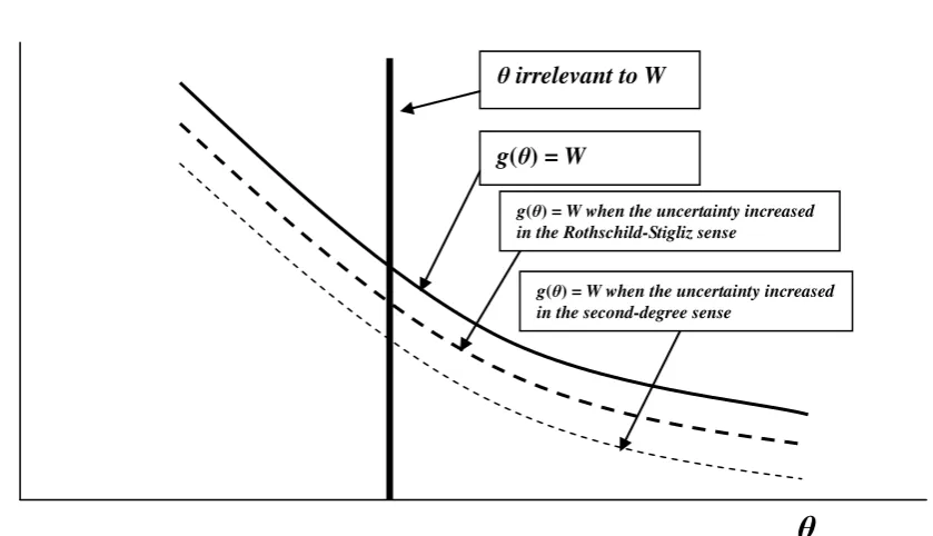
W is monotonically continuous and continuously differentiable. Because W is a sum of utilities, this property simply reflects the core idea of an endogenous RTP. However, this property is new in the sense that RTP is sensitive not only to the present utility but also to the entire stream of utility, that is, the size of the utility stream represented by the utility of steady-state consumption. This property is intuitively acceptable because it is likely that people set their principles or parameters for their behaviors considering the final consequences of their behavior (i.e., the steady state; see, e.g., Barsky and Sims, 2012).

Another essential property that must be incorporated into the model is

0



dW dθ

.

Because W E

 

u

 

c and

 

t t dc c du 

0 , RTP is inversely proportionate to c*. This property is

consistent with the findings in many empirical studies, which have shown that RTP is negatively correlated with permanent income (e.g., Lawrance, 1991).

 







 









 _

θ W θ Eu c

θ ,

 





0

 _

c u dE

dθ dW

dθ

. (15)

This model is deceptively similar to Uzawa’s endogenous RTP model (Eq. 2) and simply

replaces ct with c* and

 

t t

c du

dθ



0 with

 

 

_ 0

c u dE

dθ

. However, the two models are

completely different because of the opposite characteristics of

 

t t

c du

dθ



0 and

 

 

_ 0

c u dE

dθ

.

4.3.2 Nature of the model

The model (Eq. 3) can be regarded as successful only if it exhibits stability. In Uzawa’s model,

the economy becomes unstable if

 

t t

c du

dθ



0 is replaced with

 

t 0 t

c du

dθ _{. In this section, I}

examine the stability of the model.

4.3.2.1 Equilibrium RTP

In Ramsey-type models, such as shown in Section 2.1.3, if a constant RTP is given, the value of the marginal product of capital (i.e., the value of the real interest rate) converges to that of the given RTP as the economy approaches the steady state. Hence, when a RTP is specified at a certain value, the corresponding expected steady-state consumption is uniquely determined. Given fixed values of other exogenous parameters, any predetermined RTP has unique values of expected consumption and utility at steady state. There is a one-to-one correspondence between the expected utilities at steady state and the RTPs; therefore, the expected utility at steady state can be expressed as a function of RTP. Let

c

_x be a set of steady-state consumption levels, given a set of RTPs (θx) and other fixed exogenous parameters. The concept of θ → W

discussed above can be described as

 

θ E

 

u

 

c



W



g    , (16)

where cc_x and θθ_x. On the other hand, RTP is a continuous function of steady-state consumption as shown in Eq. (15) such that θ θ

 

W θ



E



u

 

c





. The reverse function is

 

θ E

 

u

 

c



W



h    . (17)

The equilibrium RTP is determined by the point of intersection of the two functions,

 

θ

g and h

 

θ , as shown in Figure 1. Figure 2 shows the special but conventionally assumed case for h

 

θ in which θ is not sensitive to W, and RTP is constant. There exists a point of intersection because both g

 

θ and h

 

θ are monotonically continuous for θ0.

 

θ