Munich Personal RePEc Archive
Risk Estimation when the Zero
Probability of Financial Return is
Time-Varying
Grønneberg, Steffen and Sucarrat, Genaro
BI Norwegian Business School, BI Norwegian Business School
29 October 2014
Online at
https://mpra.ub.uni-muenchen.de/81882/
Risk Estimation when the Zero Probability of Financial Return is Time-Varying∗
Steffen Grønneberg†and Genaro Sucarrat‡
First version: 29 October 2014
This version: 10th October 2017
Abstract
The probability of an observed financial return being equal to zero is not nec-essarily zero. This can be due to liquidity issues (e.g. low trading volume), market closures, data issues (e.g. data imputation due to missing values), price discreteness or rounding error, characteristics specific to the market, and so on. Moreover, the zero probability may change and depend on market conditions. In ordinary models of risk (e.g. volatility, Value-at-Risk, Expected Shortfall), however, the zero probability is zero, constant or both. We propose a new class of models that allows for a time-varying zero probability, and which nests ordi-nary models as special cases. The properties (e.g. volatility, skewness, kurtosis, Value-at-Risk, Expected Shortfall) of the new class are obtained as functions of the underlying volatility and zero probability models. For a given volatility level, our results imply that risk estimates can be severely biased if zeros are not accommodated: For rare loss events (i.e. 5% or less) we find that Conditional Value-at-Risk is biased downwards and that Conditional Expected Shortfall is biased upwards. An empirical application illustrates our results, and shows that zero-adjusted risk estimates can differ substantially from risk estimates that are not adjusted for the zero probability.
JEL Classification: C01, C22, C32, C51, C52, C58
Keywords: Financial return, volatility, zero-inflated return, Value-at-Risk, Expected
Shortfall
∗We are grateful to Christian Conrad, Christian Francq, participants at the HeiKaMEtrics Con-ference 2017 (Heidelberg), VieCo 2017 conCon-ference (Vienna), the CFE 2016 conCon-ference (Seville), the CEQURA 2016 conference (Munich), the CATE September 2016 workshop (Oslo), the CORE 50th. anniversary conference (Louvain-la-Neuve), the Maastricht econometrics seminar (May, 2016), the Uppsala statistics seminar (April 2016), the CREST econometrics seminar (February 2016), the SNDE Annual Symposium 2015 (Oslo) and the IAAE Conference 2015 (Thessaloniki) for useful comments, suggestions and questions.
†Department of Economics, BI Norwegian Business School. Email: [email protected].
Contents:
1 Introduction 2
2 Financial return with time-varying zero probability 4
2.1 The ordinary model of return . . . 4
2.2 A model of return with time-varying zero probability . . . 5
2.3 Conditional VaR . . . 6
2.4 Conditional ES . . . 9
2.5 Estimation . . . 10
3 Empirical application 12 3.1 Models. . . 12
3.2 Volatility . . . 13
3.3 Conditional VaR . . . 13
3.4 Conditional ES . . . 14
4 Conclusions 14 References 17 A Proofs 18 A.1 Proof of Proposition 1 . . . 18
A.2 Proof of Proposition 2 . . . 19
A.3 Proof of Proposition 3 . . . 19
A.4 Proof of Proposition 4 . . . 20
A.5 Proof of Proposition 5 . . . 21
A.6 Proof of Proposition 6 . . . 22
B Missing values estimation algorithm 22
1
Introduction
It is well-known that the probability of an observed financial return being equal to zero is not necessarily zero. This can be due to liquidity issues (e.g. low trading volume), market closures, data issues (e.g. data imputation due to missing values), price discreteness and/or rounding error, characteristics specific to the market, and so on. Moreover, the zero probability may change and depend on market conditions. In ordinary models of financial risk, however, the probability of a zero return is usually zero, or non-zero but constant.
Several contributions relax the constancy assumption by specifying return as a
discrete dynamic process. Hausman et al. (1992), for example, allow the zero
prob-ability to depend on other conditioning variables (e.g. volume, duration and past returns) in a probit framework. This was then extended in two different directions by
Engle and Russell (1998), and Russell and Engle (2005), respectively. In the former the durations between price increments are specified in terms of an Autoregressive Conditional Duration (ACD) model, whereas in the latter price-changes are specified in terms of an Autoregressive Conditional Multinomial (ACM) model in combination
with an ACD model of the durations between trades. Liesenfeld et al. (2006) point
in Bien et al. (2011). Rydberg and Shephard (2003) propose a framework in which the price increment is decomposed multiplicatively into three components:
Activ-ity, direction and integer magnitude. Finally, K¨umm and K¨usters (2015) propose a
zero-inflated model for German milk-based commodity returns with autoregressive persistence, where zeros occur either because there is no information available (i.e. a binary variable), or because of rounding.
Even though discrete models may in many cases provide a more accurate char-acterisation of observed returns, the most common models used in risk analysis in empirical practice are continuous. Examples include the Autoregressive Conditional
Heteroscedasticity (ARCH) class of models of Engle (1982), the Stochastic
Volatil-ity (SV) class of models (see Shephard (2005)) and continuous time models (e.g.
Brownian motion).1 Arguably, the discreteness-point that causes the biggest
prob-lem for continuous models is located at zero. This is because zero is usually the most frequently observed single value – particularly in intraday data, and because its probability is often time-varying and dependent on random or non-random events (e.g. periodicity), or both. A non-zero and/or time-varying zero probability may thus severely invalidate the parameter and risk estimates of continuous models, in partic-ular if the zero process is non-stationary. We propose a new class of financial return models that allows for a time-varying conditional probability of a zero return. The new class decomposes return multiplicatively into a continuous part, which can be specified in terms of common volatility models, and a discrete part at zero that is appropriately scaled by the zero probability. Standard volatility models (e.g. ARCH, SV and continuous time models) are therefore nested and obtained as special cases.
Hautsch et al.(2013) proposed a model for volume that uses a similar decomposition to ours. In their model the dynamics is governed by a logarithmic Multiplicative
Error Model (MEM) with a GeneralisedF as conditional density, seeBrownlees et al.
(2012) for a survey of MEMs. Our model is much more general and nests their
spec-ification as a special case: The dynamics need not be specified in logs, the density of
the continuous part (squared) need not be GeneralisedF, our framework also applies
to return models (not only MEMs), and the model class is not restricted to ARCH type models. Another attraction of our model is that many return properties (e.g. conditional volatility, return skewness, Value-at-Risk and Expected Shortfall) are ob-tained as functions of the underlying volatility model. Moreover, our model allows – in principle – for autoregressive conditional dynamics in both the zero probability and volatility specifications, and for a two-way feedback between the two.
Our results shed light on the effect and bias caused by zeros in several ways. First, for a given volatility level, our results imply that a higher zero probability increases both the skewness and kurtosis of return, but reduces return variability defined as
absolute return (see Proposition 1). Second, if the model and/or estimator used by
the practitioner does not accommodate zeros appropriately, then volatility estimates may be severely biased in unpredictable ways. This is particularly the case if the zero probability is non-stationary. To alleviate this problem we outline an estimation and inference procedure that reduces the bias caused by a time-varying zero probability (possibly non-stationary), and which can be combined with well-known models and
estimators (see Section2.5). Third, we derive general formulas for Conditional
at-Risk (VaR). For a given level of volatility, we find that risk – when defined as Conditional VaR – will be biased downwards for rare loss events (5% or less) if
zeros are not adjusted for (see Section 2.3). Fourth, we derive general formulas for
Conditional Expected Shortfall (ES). For a given level of volatility, we find that risk
– when defined as Conditional ES – will be biased upwards – i.e. the opposite of
Conditional VaR – for rare loss events (10% or less) if zeros are not adjusted for (see
Section 2.4). This may have implications for financial market supervision, due to
the increased emphasis on Expected Shortfall in the Basel III regulatory framework. Finally, an empirical illustration shows that risk estimates can be substantially biased in practice if the time-varying zero probability is not accommodated appropriately
(see Section3).
The rest of the paper is organised as follows. Section 2 presents the new model
class and derives some general properties, including the formulas for Conditional VaR and Conditional ES. The section ends by outlining a general estimation and inference procedure that reduces the biases caused by zeros, and which can be combined with
common models and methods. Section3 contains our empirical application, whereas
Section 4 concludes. The Appendix contains the proofs and additional auxiliary
material. Tables and Figures are located at the end.
2
Financial return with time-varying zero
proba-bility
2.1
The ordinary model of return
The ordinary model of a financial returnrt is given by
rt=σtwt, Et−1(wt) = 0, Et−1(w2t) = σ2w, Pt−1(wt = 0) = 0, t ∈Z, (1)
whereσt>0 is a time-varying scale or volatility (that needs not equal the conditional
standard deviation). The subscriptt−1 is notational shorthand for conditioning on
the past. Unless we state otherwise, the past will be the sigma-field generated by
{ru : u < t}, and when needed we will denote this sigma-field by Ftr−1. The wt is
an innovation andPt−1(wt= 0) is the zero probability of wt conditional on the past.
We refer to (1) as an “ordinary” model of return, since the zero probability of return
rt is 0 for all t. An example of an ordinary model is the GARCH(1,1) of Bollerslev
(1986), where
σ2t =α0+α1r2t−1 +β1σt2−1, wt ∼N(0,1). (2)
Another example is the Stochastic Volatility (SV) model, where
lnσt2 =α0 +β1lnσ2t−1+ηvt−1, wt∼N(0,1), vt∼N(0, σv2), (3)
with vi being independent of wj for all pairs i, j. Other examples of σt include
quadratic variation (e.g. Brownian motion) and other continuous time notions of
volatility, the Gaussian log-GARCH models proposed independently byGeweke(1986),
GED,2 the mixed data sampling (MIDAS) regression of Ghysels et al. (2006), and
the Dynamic Conditional Score (DCS)/Generalised Autoregressive Conditional Score
(GAS) models of Harvey(2013) and Creal et al. (2013).
2.2
A model of return with time-varying zero probability
Let{rt} denote a return process governed by
rt = σtzt, σt>0, t∈Z, (4)
zt = wtItπ1−t1/2, Et−1(wt) = 0, Et−1(w2t) =σw2, Pt−1(wt= 0) = 0, (5)
It ∈ {0,1}, π1t=Pt−1(It = 1), 0< π1t≤1. (6)
Again, the subscript t−1 is shorthand notation for conditioning on the past, and
again the past is given by the sigma-field generated by past returns, i.e. Fr
t−1. The
indicator variable It determines whether return rt is zero or not: rt 6= 0 if It = 1,
and rt = 0 if It = 0. This follows from Pt−1(wt = 0) = 0, which is an assumption
needed for identification (it ensures zeros do not originate from both wt and It).
The probability of a zero return conditional on the past is thus π0t = 1−π1t. The
motivation for lettingπ1tenter the way it does in zt is to ensure thatV art−1(z) =σw2
(see Proposition 1 below). It should be underlined that (4) – (6) do not exclude
the possibility ofIt being contemporaneously dependent on the value of wt, e.g. that
small values of |wt| increases the probability of It being zero. A specific example is
the situation where It = 1 if |wt| <0.05 and 0 otherwise, and where wt conditional
on the past is standard normal (in this specific exampleπ1t = 0.96). It should also be
underlined that (4) – (6) do not exclude the possibility ofσtbeing contemporaneously
dependent on wt or It, or both. Finally, we will refer to ert=σtwt as “zero-adjusted”
return, sinceret=rtπ11t/2 whenever It 6= 0.
An attractive feature of (4)–(6) is that many properties can be expressed as a
function of the underlying models of volatility and zero probability. In deriving these properties we rely on suitable subsets of the following assumptions.
Assumption 1 (regularity of distribution). Conditional on the past Fr t−1:
(a) The joint probability distribution of wt and It is regular.
(b) The joint probability distribution ofret and It is regular.
Assumption 2 (identification). For all t: Et−1(wt|It = 1) = 0 and Et−1(wt2|It =
1) =σ2
w with 0< σ2w <∞.
Assumption 1 is a technical condition that ensures probabilities conditional on the
past can be manipulated as usual, seeShiryaev (1996, pp. 226-227). (a) will usually
be needed when deriving properties involvingzt, whereas (b) will usually be needed
when deriving properties involvingrt. Assumption 2states that, conditional on both
Fr
t−1 and It = 1, the expectation of wt is zero, and the expectation of wt2 exists
and is equal to σ2
w for all t. The motivation behind this assumption is to ensure
that zt exhibits the first and second moment properties typically possessed by the
scaled innovation in volatility models. The assumption can thus be viewed as an identification condition. The zero-mean property will usually ensure that returns
are Martingale Difference Sequences (MDSs), and most commonlyσ2
w = 1, as in the
ARCH class of models. It should be noted, however, that Assumption2is only needed
in Proposition1. This proposition collects some properties that follow from (4) – (6)
together with some additional moment assumptions.
Proposition 1. Suppose (4) – (6), Assumption 1(a) and Assumption 2 hold. Then:
(i) IfEt−1|zt|<∞ for all t, then {zt} is a Martingale Difference Sequence (MDS).
(ii) IfEt−1|zt2|<∞ for all t, thenV art−1(zt) = σw2 for allt, and{zt}is
covariance-stationary with E(zt) = 0, V ar(zt) = σw2 and Cov(zt, zt−j) = 0 when j 6= 0.
(iii) If Et−1|zst|<∞ for some s≥0, then Et−1(zts) = π
(2−s)/2
1t Et−1(wst|It= 1).
(iv) If Et−1|zst|<∞ for some s≥0, then Et−1|zt|s =π(21t−s)/2Et−1(|wt|s|It= 1).
Proof: See Appendix A.1.
Property (i) means {zt} is an MDS even if π1t is time-varying. Indeed, it remains
an MDS even if {It} is non-stationary. Usually, (i) will imply that {rt} is also an
MDS, e.g. in the ARCH class of models, since there Et−1(rt) =σtEt−1(zt). Property
(ii) means σ2
t corresponds to the conditional variance in ARCH models, and that
the unconditional second moment – if it exists – is not affected by the presence of time-varying zero probability. For example, in the semi-strong GARCH(1,1) of
Hansen (1994), where zt is strictly stationary and ergodic with σt2 = α0+α1r2t−1 +
β1σ2t−1, we have V art−1(rt) = σt2 and V ar(rt) = α0/(1 −α1 − β1) regardless of
whether π1t is constant or time-varying. If zt is not strictly stationary, e.g. because
the zero probability is periodic (this is common in intraday returns), then Property
(ii) meansztwill still be covariance stationary. Property (iii) means higher order (i.e.
s > 2) conditional moments (in absolute value) are scaled upwards by positive zero
probabilities, whereas the opposite is the case for lower order (i.e.s <2) conditional
moments. In particular, both conditional skewness (s = 3) and conditional kurtosis
(s = 4) become more pronounced. Similarly, property (iv) means higher order (i.e.
s >2) conditional absolute moments are scaled upwards by positive zero probabilities,
whereas the opposite is the case for lower order (i.e.s <2) conditional moments. For
a given volatility level σt, this means the conditional absolute return (i.e. s = 1) is
scaled downwards, sinceE|x|s< E|x|2 for 0< s <2 due to the Lyapounov inequality.
2.3
Conditional VaR
For notational simplicity we will henceforth denote the cumulative density function
(cdf) of a random variable Xt at t conditional on Ftr−1 as FXt(x), hence omitting
the subscript t−1. Conditional on both Fr
t−1 and It = 1, we will use the notation
FXt|1(x).
Proposition 2 (cdfs of zt and rt). Suppose (4) – (6) hold, and let 1{x≥0} denote an
(i) If also Assumption 1(a) holds, then the cdf of zt at t conditional on Ftr−1 is
Fzt(x) = Fwt|1(xπ 1/2
1t )π1t+ 1{x≥0}(1−π1t). (7)
(ii) If also Assumption 1(b) holds, then the cdf of rt at t conditional on Ftr−1 is
Frt(x) = Fert|1(xπ 1/2
1t )π1t+ 1{x≥0}(1−π1t). (8)
Proof: See Appendix A.2.
Natural examples ofFwt|1 and Fert|1, respectively, are N(0,1) and N(0, σ
2
t).
If FXt(x) denotes the cdf of a random variable Xt conditional on the past F
r t−1,
then its lower c-quantile with c∈(0,1) is given by
Xc,t= inf{x∈R:FXt(x)≥c}. (9)
We will writeFX−t1(c) = Xc,t even though the inverse ofFX does not exist, and we will
refer to F−1
Xt(c) as the generalised inverse of FXt(x), see e.g. Embrechts and Hofert
(2013). In order to derive general formulas for quantiles and conditional VaRs, we
introduce an additional, technical assumption on the distributions of wt and er. The
assumption can be relaxed, but at the cost of more complicated formulas.
Assumption 3. Conditional on the past Fr
t−1 and It= 1:
(a) The cdf of wt, denoted Fwt|1, is strictly increasing. (b) The cdf of ert, denoted Fret|1, is strictly increasing.
The assumption is fairly mild, since it holds for most of the conditional densities that
have been used in the literature, including the standard normal, the Student’st and
the GED, and also for many skewed versions. In particular, the assumption does not
require smoothness nor continuity. A consequence of (a) and (b) is that Fzt and Frt
are both increasing. Accordingly, their lower and upper c-quantiles – as defined in
Acerbi and Tasche (2002, Definition 2.1, p. 1489) – coincide. This will simplify the conditional quantile, VaR and ES expressions.
Proposition 3 (conditional quantiles and VaRs). Suppose (4) – (6) hold and that
c∈(0,1):
(a) If also Assumptions 1(a) and 3(a) hold, then the cth. quantile of zt conditional
on the past Fr
t−1 is
zc,t = Fz−1(c)
=
π1−t1/2Fw−t1|1(c/π1t) if c < Fwt|1(0)π1t
0 if Fwt|1(0)π1t ≤c < Fwt|1(0)π1t+π0t
π1−t1/2Fw−t1|1h(c−π0t)
π1t
i
if c≥Fwt|1(0)π1t+π0t,
(10)
(b) If also Assumptions 1(b) and 3(b) hold, then the cth. quantile of rt conditional
on the past Fr
t−1 is
rc,t = Fr−1(c)
=
π1−t1/2Fer−t|11(c/π1t) if c < Fret|1(0)π1t
0 if Fert|1(0)π1t ≤c < Fert|1(0)π1t+π0t
π1−t1/2Fer−t|11h(c−π0t)
π1t
i
if c≥Fert|1(0)π1t+π0t,
(11)
and the (100·c)% Value-at-Risk (VaRc) ofrtconditional on the past Ftr−1 is−rc,t.
Proof: See Appendix A.3.
The expression for rc,t is not necessarily the most convenient from a practitioner’s
point of view. Indeed, in some situations it is desirable to be able to writerc,t=σtzc,t,
so that estimation of σt and zc,t may be separated into two different steps. The
following assumption, which is fulfilled by most ARCH models but not necessarily by
SV models, ensuresrc,t can indeed be written as σtzc,t.
Assumption 4. σt is measurable with respect to Ftr−1.
Proposition 4. Suppose (4) – (6) and Assumptions 1, 3 and 4 hold. If c ∈ (0,1), then rc,t =σtzc,t, where zc,t is given by (10).
Proof: See Appendix A.4
It should be noted that we need both the (a) and (b) parts of Assumptions1 and 3
for the proposition to hold.
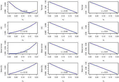
Figures 1and 2provide an insight into the effect of zeros on Conditional VaR for
a fixed value of volatility σt. Figure 1 plots Conditional VaR (i.e. −zc,t) for
differ-ent values of c and π0t, and for four different densities of wt: The standard normal,
the standardised skew normal, the standardised Student’s t with five degrees of
free-dom, and the standardised skew Student’s t with five degrees of freedom.3 When
c ∈ {0.05,0.01}, then Conditional VaR always increases when the zero probability
π0t increases. By contrast, when c= 0.10 then Conditional VaR generally falls, the
exception being when wt ∼N(0,1). There, Conditional VaR first falls and then
in-creases in π0t. In summary, therefore, the main implication of Figure 1 is that the
effect of zeros on conditional VaR, for a given level of volatility, is highly non-linear
and dependent on the density of wt. Nevertheless, if c is sufficiently small, then
the Figure suggests Conditional VaR usually increases when the zero probability in-creases. In other words, if the estimation of Conditional VaR is not adjusted for the zero probability, then the estimate of risk – defined in terms of Conditional VaR –
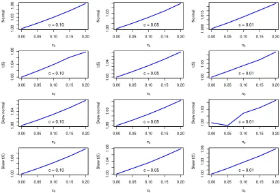
will be biased downwards. Figure 2 provides an insight into the relative size of the
bias. The Figure contains plots of the ratio of the unadjusted Conditional VaR (nu-merator) versus the zero-adjusted Conditional VaR (denominator). The unadjusted
Conditional VaRs are those ofwt(i.e. those ofzt under the assumption thatπ1t= 1),
whereas the zero-adjusted Conditional VaRs are those of Figure 1. The plot reveals
that, in relative terms, the effect depends in non-linear ways onc,π0tand the density
ofwt. Nevertheless, one general characteristic is that, when c= 0.01, then the largest
effect onzc,t (and hence conditional VaR) occurs whenwtis normal and skew normal.
That is, the most commonly used density assumption.
2.4
Conditional ES
Let FX(x) and Xc denote the cdf and c-quantile of a random variable X, and let
1{X<Xc} denote an indicator function equal to 1 ifX < xc and 0 otherwise. Following
Acerbi and Tasche (2002, Definition 2.6, p. 1491), we define the Expected Shortfall
at levelc∈(0,1) for a random variable X as
ESc =−
1
c
E(X1{X<Xc}) +Xc(c−FX(Xc))
. (12)
The last term in the definition, i.e.Xc(c−FX(Xc)), is needed ifFX is discontinuous.
This may complicate the expressions for ESc considerably. As a mild simplifying
assumption, therefore, we introduce a continuity assumption onFwt|1andFert|1, which
ensures that the term is zero forFzt and Frt.
Assumption 5. Conditional on the past Fr
t−1 and It= 1:
(a) The cdf ofwt, denotedFw|1, is continuous and has density with respect to Lebesgue
measure.
(b) The cdf ofret, denotedFert|1, is continuous and has density with respect to Lebesgue measure.
The assumption is mild in the sense that it is fulfilled in most of the empirical applications that compute VaR and ES. That the assumption indeed ensures that
Xc(c−FX(Xc)) is zero for both zt and rt, is showed in Appendix A.5 (see Lemma
2).
Proposition 5. Suppose (4) – (6) hold and that c∈(0,1):
(a) If also Assumptions1(a),3(a) and5(a) hold, then the(100·c)% Expected Shortfall
(ESc) of zt conditional on the past Ftr−1 is −c−1Et−1(zt|zt ≤zc,t), where
Et−1(zt|zt ≤zc,t)
=
π1tEt−1
wt1{wt≤Fw−|11(c/π1t)}
if c < Fw|1(0)π1t,
π1tEt−1 wt1{wt≤0}
if Fw|1(0)π1t≤c < Fw|1(0)π1t+π0t,
π1tEt−1
wt1{wt≤Fw−|11[(c−π0t)/π1t]}
if c≥Fw|1(0)π1t+π0t,
(13)
(ESc) of rt conditional on the past Ftr−1 is −c−1Et−1(rt|rt≤rc,t), where
Et−1(rt|rt ≤rc,t)
=
π1tEt−1
e
rt1{ert≤Fer−|11(c/π1t)}
if c < Fer|1(0)π1t,
π1tEt−1 ert1{ert≤0}
if Fer|1(0)π1t≤c < Fre|1(0)π1t+π0t,
π1tEt−1
e
rt1{ert≤Fre−|11[(c−π0t)/π1t]}
if c≥Fer|1(0)π1t+π0t,
(14)
Proof: See Appendix A.5.
Just as for the expression for the quantile rc,t in Proposition 3, the expression for
Et−1(rt|rt≤rc,t) is not necessarily the most convenient from a practitioner’s point of
view. Indeed, in many situations it would be desirable if we could write Et−1(rt|rt ≤
rc,t) as σtEt−1(zt|zt ≤ zc,t), so that estimation of σt and Et−1(zt|zt ≤ zc,t) may be
separated into two different steps. If we rely on all the assumptions stated so far,
apart from Assumption2, then we can indeed write the expression in this way.
Proposition 6. Suppose (4) – (6), and Assumptions 1 and 3 – 5 hold. If c∈(0,1), thenEt−1(rt|rt≤rc,t) = σtEt−1(zt|zt≤zc,t), whereEt−1(zt|zt ≤zc,t) is given by (13).
Proof: See Appendix A.6.
For a given volatility levelσt, Conditional ES is determined by−π1tc−1Et−1(zt|zt ≤
zc,t). Figure 3 plots this expression for different values of c and π0t, and for
dif-ferent conditional densities of wt (the same as those for Conditional VaR above).
Contrary to the Conditional VaR case, here the effect is always monotonous for
c ∈ {0.10,0.05,0.01} albeit opposite to that of Conditional VaR: Conditional ES
falls as the zero probability increases. In other words, risk – defined as Conditional
ES – will be biased upwards if not adjusted for the zero probability. Figure4provides
insight into the magnitude of bias in relative terms. The plots contain the ratio of unadjusted Conditional ES (numerator) versus the zero-adjusted Conditional ES
(de-nominator). The unadjusted ones are computed under the assumption that π1t = 1,
whereas the zero-adjusted ones are those of Figure3. The plot reveals that, in relative
terms, the largest effect occurs whenc= 0.10 andwt is skewt. Also, contrary to the
Conditional VaR case, the normal and skew normal densities produce the smallest biases in relative terms.
2.5
Estimation
Theσtcan be specified in terms of a wide range of volatility models. If{zt}is strictly
stationary and ergodic, for example, then the result by Lee and Hansen (1994) means
σt can be specified as a GARCH(1,1) in the usual way, i.e.
σt2 =α0+α1r2t−1+β1σt2−1, (15)
since Gaussian QML then provides strongly consistent and asymptotically normal
estimates ofα0, α1 and β1. Escanciano (2009) and Francq and Thieu (2015) extend
particular, the latter accommodates asymmetry (i.e. “leverage”) and stationary
co-variates (‘X’), including past values ofIt, as conditioning variables. Another example
of σt with zt stationary is a log-GARCH(1,1) that “skips” the zeros, i.e.
lnσt2 =α0+α1It−1lnrt2−1+β1lnσt2−1, (16)
where Itlnrt2 = lnrt2 if It = 1 and 0 otherwise. A MEM version of this specification
was proposed by Hautsch et al. (2013) for volume, and Francq and Zako¨ıan (2017)
show that an extended version of the specification is strictly stationary and ergodic.
If the zero-process{It}is not stationary, however, thenztis not strictly stationary.
The zero-process can be non-stationary if, say, the zero probability is periodic (as in intraday returns), or if it is trending downwards over time because of general market developments (e.g. the influx of high-frequency algorithmic trading, increased trading volume, increased quoting frequency, lower tick-size, etc.). In this case, an alternative
approach to the specification ofσt is to formulate it in terms of zero-adjusted return
e
rt =σtwt. For example, the GARCH(1,1) model in terms of zero-adjusted return is
given by
σt2 =α0+α1ert2−1+β1σt2−1, (17) whereas the zero-adjusted log-GARCH(1,1) model is given by
lnσ2t =α0+α1lnert2−1+β1lnσ2t−1. (18)
If ert were observed, then estimation could proceed as usual by, say, maximising
Pn
t=1lnfert(ert), where fert is a suitably chosen density. The approximate estimation
and inference procedure we propose consists of first replacing ret with its estimate
rtbπ11t/2, and then to treat zeros as “missing”:
1. Record the locations at which the observed return rt is zero and non-zero,
respectively. Use these locations to estimate π1t.
2. Obtain an estimate ofretby multiplyingrtwithbπ11t/2, wherebπ1tis the fitted value
of π1t from Step 1. At zero locations the zero-adjusted return ret is unobserved
or “missing”.
3. Use an estimation procedure that handles missing values to estimate the volatil-ity model.
Sucarrat and Escribano(2017) propose an algorithm of this type for the log-GARCH model, where missing values are replaced by estimates of the conditional expectation. If Gaussian (Q)ML is used for estimation, then this can be viewed as a dynamic variant of the Expectation Maximisation (EM) algorithm. A similar algorithm can be devised for many additional volatility models, including the GARCH model, subject
to suitable assumptions. Appendix B contains the details of the algorithm together
with a small simulation study, whereas Section 3 applies the algorithm to the daily
Apple return series. It should be noted that the algorithm does not necessarily provide consistent parameter estimates – in particular if the zero probability is large. The reason for this is that the missing values induces a repeated invertibility or irrelevance
3
Empirical application
In order to shed light on how returns with time-varying zero probabilities affect volatility dynamics, Value-at-Risk and Expected Shortfall in practice, we revisit three
of the return series in Sucarrat and Escribano (2017). These series are of interest,
since they exhibit a variety of zero-dynamics characteristics. The three series are the daily Standard and Poor’s 500 stock market index (SP500) return, the daily Ekornes stock price return and the daily Apple stock price return. The first and third return series are well-known, whereas the second is a leading Nordic furniture manufacturer listed on the Oslo Stock Exchange. Ekornes is a medium-sized company in international terms, since its market value is approximately 300 million euros (at the end of the series). Our interest in Ekornes is mainly due to its relatively large – for daily returns – proportion of zeros over the sample (about 19%). The source
of the data is Yahoo Finance (http://finance.yahoo.com). All three returns are
computed as (lnSt−lnSt−1)·100, whereSt is the index level or stock price at dayt.
Saturdays and Sundays, where returns are usually 0, are not included in our sample.
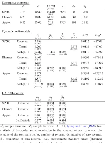
Descriptive statistics are contained in the upper part of Table1. The statistics confirm
that the returns exhibit the usual properties of excess kurtosis compared with the normal, and ARCH as measured by first order serial correlation in the squared return. The number of zeros varies from only 2 observations (about 0.1% of the sample) for SP500 to 667 observations (about 19% of the sample) for Ekornes.
3.1
Models
The middle part of Table1contains estimates of three dynamic logit models for each
return:
Constant: ht = ρ0,
Trend: ht = ρ0+λt∗, t∗ =t/n, t∗ ∈(0,1],
ACL(1,1): ht = ρ0+ρ1st−1+ζ1ht−1.
The conditional zero probability π0t is thus given by (1 −π1t) with π1t = 1/(1 +
exp(−ht)). In the first model the zero probability is constant, in the second it is
governed by a deterministic trend (t∗ is “relative time”) and in the third is a first
order Autoregressive Conditional Logit (ACL). The ACL is the binomial version of
the Autoregressive Conditional Multinomial (ACM) ofRussell and Engle(2005). For
SP500 returns, it is the first logit specification that fits the data best according to the
Schwarz (1978) information criterion (SIC), whereas for Apple and Ekornes returns
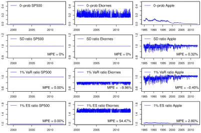
the best model according to SIC is the ACL(1,1). The first row of Figure 5contains
the fitted zero probabilities. For SP500 and Ekornes the series appear to be stationary, whereas for Apple the series appear to be downward trending over the sample and hence non-stationary.
The bottom part of Table 1 contains GARCH(1,1) estimates of the return series.
In the SP500 and Ekornes cases we fit a single specification, namely
Ifztis (strictly) stationary (and ergodic), then the results by Escanciano(2009), and
Francq and Thieu (2015) imply that Gaussian QML provides consistent parameter estimates (subject to additional conditions). In the Apple case we fit two different
GARCH(1,1) specifications, namely (19) and a zero-adjusted specification:
0-adj: σ2t =α0+α1ert2−1+β1σt2−1. (20)
The zero-adjusted specification is estimated by Gaussian QML in combination with
the missing values algorithm proposed in Sucarrat and Escribano (2017), since It
appears to be non-stationary with a downwards trend over the sample in the zero
probability. To recall (see Section 2.5), the algorithm proceeds by replacing ert with
its estimate bπ11t/2rt whenever rt 6= 0, while treating zeros as missing observations.
Next, the missing values are replaced by estimates of their conditional expectations,
i.e. Ebt−1(ret2) = bσt2. Since Gaussian QML is used for estimation, the algorithm can
be viewed as a dynamic variant of the Expectation-Maximisation (EM) algorithm
(see Appendix B for more details). The nominal differences between the parameter
estimates of the Ordinary and 0-adj specifications appear small. However, as we will see shortly, these small nominal differences – together with the different treatment of zeros – can lead to substantially different risk estimates and risk dynamics.
3.2
Volatility
The second row in Figure 5 contains graphs of the ratios of the fitted conditional
standard deviations. For SP500 and Ekornes estimates ofσt are unaffected by zeros
(subject to the assumption that zt is strictly stationary and ergodic), so the ratios
are 1 over the whole sample. For Apple the ratio is computed as bσt/bσt,0-adj, i.e. the
fitted values of (19) over those from the 0-adjusted specification, i.e. (20). The Mean
Percentage Error (MPE), computed asn−1Pn
t=1(xt−1)·100 wherext=bσt/bσt,0-adj is
the ratio at t, provides an overall measure of relative difference. Of course, the MPE
is by construction 0% for SP500 and Ekornes. For Apple the MPE is 0.32%, which suggests volatility on average is only 0.32% higher than zero-adjusted volatility. A closer inspection, however, reveals that volatility is biased downwards in the beginning of the sample, and biased upwards towards the end. Also, the day-to-day difference between the two measures vary much more in the beginning, when there are more zeros, than towards the end. Finally, the difference in percentage terms is relatively low towards the end of the sample.
3.3
Conditional VaR
To illustrate the effect of zeros on Conditional VaR, we choose c = 0.01. Ratios of
the estimated Conditional VaRs are contained in the third row of graphs in Figure5,
and the ratio attis given byxt=brc,t/brc,t,0−adj. For SP500, Ekornes and Apple,brc,t is
computed asbσtzbc, wherebσtis the fitted value of (19), andzbcis the empiricalc-quantile
of the residualszbt. For SP500 and Ekornes, brc,t,0−adj is computed as bσtbzc,t, where bzc,t
is obtained using the relevant formula in (10), i.e. π−1t1/2Fw−|11(c/π1t). To estimate
Fw−|11(c/π1t) att we use the empirical c/bπ1t-quantile of the zero-adjusted residuals wbt
fitted value of (20), and bzc,t is computed in the same way as for SP500 and Ekornes.
Again we use the MPE (= n−1Pn
t=1(xt−1)·100) as an overall measure of relative
difference. Unsurprisingly, the MPE is essentially 0% for SP500. For Ekornes, by
contrast, the MPE is about −10%. This means risk defined as Conditional VaR, on
average, is biased downwards by 10% if zeros are not adjusted for. For Apple the
MPE is only −0.40%, which suggests the downward bias is low. However, recalling
that the zero probability has been gradually declining over the sample, a closer look reveals that the Conditional VaR is biased downwards in the first part of the sample – at times more than 10%, and biased upwards towards the end – always below 5%. The graph also shows that the ratio is more variable when there are more zeros, i.e. in the beginning of the sample.
3.4
Conditional ES
To illustrate the effect of zeros on Conditional ES, we choose c = 0.01 also here.
Ratios of the estimated Conditional ESs are contained in the bottom row of graphs
in Figure5, and the ratio at t is given by xt=EScc,t/EScc,t,0−adj. For SP500, Ekornes
and Apple, EScc,t is computed as −c−1σbtEbt−1(zt|zt ≤ zc,t), where bσt is the estimate
from (19), and Ebt−1(zt|zt ≤ zc) is computed as the sample average of the residuals
b
zt that are equal to or lower than zbc as defined above (i.e. the empirical c-quantile
of the residualszbt). For SP500 and Ekornes, the zero-adjusted estimateEScc,t,0−adj is
computed as−c−1σb
tEbt−1(zt|zt≤zc,t), where Ebt−1(zt|zt≤zc,t) is equal to the relevant
formula in (13), i.e.π1tEt−1
wt1{wt≤Fwt−1|1(c/π1t)}
. As for Conditional VaR, to estimate
Fw−t1|1(c/π1t) at t we use the empirical c/bπ1t-quantile of the zero-adjusted residuals wbt
(zeros excluded). Next, we estimate Et−1
wt1{wt≤F−
1
wt|1(c/π1t)}
at t by forming an
average made up of the non-zero residuals wb: n−11PIt=1wbt1{wbt≤Fb−1
wt|1(c/πb1t)}, where
n1 is the number of non-zero observations (i.e. n1 = Pnt=1It), Fbw−t1|1(c/πb1t) is the
estimate ofFw−t1|1(c/π1t), and the symbolismPIt=1 means the summation is over
non-zero values only. For Apple, EScc,t,0−adj is computed as −c−1bσt,0−adjEbt−1(zt|zt≤zc,t),
where bσt,0−adj is the estimate from (20), and where Ebt−1(zt|zt ≤ zc,t) is computed in
the same way as for SP500 and Ekornes. The graphs ofxt and the MPEs show that
Conditional ES is biased upwards in the Ekornes and Apple cases, and much more so than for VaR. Indeed, for Ekornes Conditional ES is on average biased upwards by about 54%, which is huge. Usually, daily stock returns will not exhibit a zero probability of about 19%, as in the Ekornes case. Usually, they will be below 5%. Nevertheless, the results do suggest the effect of zeros is much higher on Conditional
ES than on Conditional VaR. Finally, also here does the graph ofxtfor Apple exhibit
a trend over the sample due to the downwards trend in the zero probability.
4
Conclusions
new class is that standard volatility models (e.g. ARCH, SV and continuous time models) are nested and obtained as special cases, and that the properties of the new class (e.g. conditional volatility, skewness, kurtosis, Value-at-Risk, Expected Shortfall, etc.) are obtained as functions of the underlying volatility model. Our results imply that, for a given volatility level, more zeros increases the skewness and kurtosis of return, but reduces return variability when defined as absolute return. Moreover, for a given level of volatility and sufficiently rare loss events (5% or less), risk defined as Conditional VaR will be biased downwards if zeros are not adjusted for, and risk defined as Conditional ES will be biased upwards if zeros are not adjusted for. The effect of zeros on volatility estimates will depend on the exact volatility model, the conditional density of return and on whether the zero probability is stationary or not. To alleviate the unpredictable biases caused by non-stationary zero processes, we outline an approximate estimation and inference procedure that can be combined with standard volatility models and estimators. Finally, our empirical illustration shows that risk estimates can be substantially biased in practice if the time-varying zero probability is not accommodated appropriately.
Our results have several practical and theoretical implications. First, our results suggests more attention should be paid to how market quotes and transaction prices are aggregated in order to compute the asset prices reported by data-providers, Cen-tral Banks and others. In particular, if a non-stationary zero process is the result of specific data practices, then it may be worthwhile to re-consider these. Second, for rare loss events we find that Conditional ES is biased upwards – sometimes substan-tially – if the zero probability is not adjusted for. This may have implications for the supervision of financial institutions, since recent regulatory changes emphasise the importance of ES (rather than VaR).
References
Acerbi, C. and D. Tasche (2002). On the coherence of expected shortfall. Journal of
Banking and Finance 26, 1487–1503.
Bauwens, L., C. Hafner, and S. Laurent (2012). Handbook of Volatility Models and
Their Applications. New Jersey: Wiley.
Bien, K., I. Nolte, and W. Pohlmeier (2011). An inflated multivariate integer count
hurdle model: an application to bid and ask quote dynamics. Journal of Applied
Econometrics 26, 669–707.
Bollerslev, T. (1986). Generalized autoregressive conditional heteroscedasticity.
Jour-nal of Econometrics 31, 307–327.
Brownlees, C., F. Cipollini, and G. Gallo (2012). Multiplicative Error Models. In
L. Bauwens, C. Hafner, and S. Laurent (Eds.), Handbook of Volatility Models and
Their Applications, pp. 223–247. New Jersey: Wiley.
Creal, D., S. J. Koopmans, and A. Lucas (2013). Generalized Autoregressive Score
Embrechts, P. and M. Hofert (2013). A note on generalized inverses. Mathematical
Methods of Operations Research 77(3), 423–432.
Engle, R. (1982). Autoregressive Conditional Heteroscedasticity with Estimates of
the Variance of United Kingdom Inflations. Econometrica 50, 987–1008.
Engle, R. F. and J. R. Russell (1998). Autoregressive Conditional Duration: A New
Model of Irregularly Spaced Transaction Data. Econometrica 66, 1127–1162.
Escanciano, J. C. (2009). Quasi-maximum likelihood estimation of semi-strong
GARCH models. Econometric Theory 25, 561–570.
Fern´andez, C. and M. Steel (1998). On Bayesian Modelling of Fat Tails and Skewness.
Journal of the American Statistical Association 93, 359–371.
Francq, C. and G. Sucarrat (2017). An Equation-by-Equation Estimator of a
Multi-variate Log-GARCH-X Model of Financial Returns. Journal of Multivariate
Anal-ysis 153, 16–32.
Francq, C. and L. Q. Thieu (2015). Qml inference for volatility models with covariates.
http://mpra.ub.uni-muenchen.de/63198/.
Francq, C., O. Wintenberger, and J.-M. Zako¨ıan (2013). GARCH Models Without
Positivity Constraints: Exponential or Log-GARCH?Journal of Econometrics 177,
34–36.
Francq, C. and J.-M. Zako¨ıan (2017). GARCH Models. New York: Marcel Dekker.
2nd. Edition, in press.
Geweke, J. (1986). Modelling the Persistence of Conditional Variance: A Comment.
Econometric Reviews 5, 57–61.
Ghysels, E., P. Santa-Clara, and R. Valkanov (2006). Predicting volatility: getting
the most out of return data sampled at different frequencies. Journal of
Economet-rics 131, 59–95.
Harvey, A. C. (2013). Dynamic Models for Volatility and Heavy Tails. New York:
Cambridge University Press.
Hausman, J., A. Lo, and A. MacKinlay (1992). An ordered probit analysis of
trans-action stock prices. Journal of financial economics 31, 319–379.
Hautsch, N., P. Malec, and M. Schienle (2013). Capturing the zero: a new class of
zero-augmented distributions and multiplicative error processes. Journal of
Finan-cial Econometrics 12, 89–121.
K¨umm, H. and U. K¨usters (2015). Forecasting zero-inflated price changes with a
markov switching mixture model for autoregressive and heteroscedastic time series.
Liesenfeld, R., I. Nolte, and W. Pohlmeier (2006). Modelling Financial Transaction
Price Movements: A Dynamic Integer Count Data Model.Empirical Economics 30,
795–825.
Ljung, G. and G. Box (1979). On a Measure of Lack of Fit in Time Series Models.
Biometrika 66, 265–270.
Milhøj, A. (1987). A Multiplicative Parametrization of ARCH Models. Research Report 101, University of Copenhagen: Institute of Statistics.
Nelson, D. B. (1991). Conditional Heteroskedasticity in Asset Returns: A New
Ap-proach. Econometrica 59, 347–370.
Pantula, S. (1986). Modelling the Persistence of Conditional Variance: A Comment.
Econometric Reviews 5, 71–73.
R Core Team (2014). R: A Language and Environment for Statistical Computing.
Vienna, Austria: R Foundation for Statistical Computing.
Russell, J. R. and R. F. Engle (2005). A Discrete-State Continuous-Time Model
of Financial Transaction Prices and Times: The Autoregressive Conditional
Multinomial-Autoregressive Conditional Duration Model. Journal of Business and
Economic Statistics 23, 166–180.
Rydberg, T. H. and N. Shephard (2003). Dynamics of Trade-by-Trade Price
Move-ments: Decomposition and Models. Journal of Financial Econometrics 1, 2–25.
Schwarz, G. (1978). Estimating the Dimension of a Model.The Annals of Statistics 6,
461–464.
Shephard, N. (2005). Stochastic Volatility: Selected Readings. Oxford: Oxford
Uni-versity Press.
Shiryaev, A. N. (1996). Probability. Springer-Verlag, New York,.
Shorack, G. and J. Wellner (1986).Empirical Processes with Applications to Statistics.
Wiley.
Sucarrat, G. and ´A. Escribano (2017). Estimation of Log-GARCH Models in the
Presence of Zero Returns. European Journal of Finance. http://dx.doi.org/10.
1080/1351847X.2017.1336452.
Sucarrat, G., S. Grønneberg, and ´A. Escribano (2016). Estimation and Inference in
Univariate and Multivariate Log-GARCH-X Models When the Conditional Density
A
Proofs
A.1
Proof of Proposition
1
(i) Assumption2 and Et−1|zt|<∞imply that
Et−1(zt) = π1−t1/2Et−1(wtIt) (21)
= π1−t1/2Et−1(wt·1|It= 1)π1t+Et−1(wt·0|It= 0)π0t
(22)
= 0 (23)
for all t. Note that the notation Et−1(wt·0|It = 0)π0t stands for Et−1(wt·0)
whenever π0t = 0. Accordingly, {zt} is an MDS.
(ii) Assumption2 and Et−1|z2t|<∞ imply that
Et−1(zt2) = π1−t1Et−1(wt2It2) (24)
= π−1t1Et−1(w2t ·1|It= 1)π1t+Et−1(wt2·0|It= 0)π0t
(25)
= π−1t1σw2π1t
(26)
= σ2w. (27)
for all t. Note that also here the notation Et−1(wt2 · 0|It = 0)π0t stands for
Et−1(w2t ·0) whenever π0t = 0. Next, since{zt}is an MDS and V art−1(zt) =σw2
for all t, we have (for allt) that E(zt) = 0, E(zt2) =σw2 and Cov(zt−i, zt−j) = 0
for all i6=j. So {zt}is covariance-stationary.
(iii) Since Et−1|zst|<∞, we have that
Et−1(zts) = π
−s/2
1t Et−1(wstIt) (28)
= π−1ts/2Et−1(wts·1|It= 1)π1t+Et−1(wst ·0|It= 0)π0t
(29)
= π(21t−s)/2Et−1(wst|It= 1) (30)
for all t. Again, the notation Et−1(wts ·0|It = 0)π0t stands for Et−1(wst · 0)
whenever π0t = 0.
(iv) Since If Et−1|zts|<∞, we have that
Et−1|zt|s = π1−ts/2Et−1(|wt|sIts) (31)
= π1−ts/2Et−1(|wt|s·1|It = 1)π1t+Et−1(|wt|s·0|It = 0)π0t
(32)
= π1(2t−s)/2Et−1(|wt|s|It= 1) (33)
for all t. Again, the notation Et−1(|wt|s·0|It = 0)π0t stands for Et−1(|wt|s·0)
A.2
Proof of Proposition
2
Let Xt = wtItπ1−t1/2, and let Pt−1(Xt ≤ x) denote the cdf of Xt at t conditional on
Fr
t−1. By Assumption1(a) this conditional probability is regular. Hence:
Pt−1(Xt≤x) = Pt−1(wtItπ−1t1/2 ≤x)
(a)
= Pt−1(wtItπ−1t1/2 ≤x, It= 1) +Pt−1(wtItπ1−t1/2 ≤x, It = 0)
(b)
= Pt−1(wtπ1−t1/2 ≤x, It = 1) +Pt−1(0≤x, It= 0)
(c)
= Pt−1(wtπ−1t1/2 ≤x, It = 1) + 10≤xπ0t
= Pt−1(wtπ−1t1/2 ≤x|It= 1)π1t+ 10≤xπ0t
= Pt−1(wt ≤x√π1t|It= 1)π1t+ 10≤xπ0t
(d)
= Fwt|1(x
√
π1t)π1t+ 10≤xπ0t,
where we have used (a) P(A) = P(A∩B) +P(A∩Bc), (b) I
t = 1 in wtItπ1−t1/2 in
the first term andIt= 0 in the second, (c) for 0> x we have Pt−1(0≤x∩It = 0) =
Pt−1(∅∩It = 0) = 0, and for 0≤xwe havePt−1(0≤x, It= 0) =Pt−1(Ω∩{It = 0}) =
Pt−1(It = 0) =π0t, where Ω is the whole outcome set of the underlying probability
space, (d) the assumption π1t = Pt−1(It = 1) in (6) implies that π1t is measurable
with respect toFr
t−1.
Replacing wt with ert so that Xt = rt, and assuming Assumption 1(b) instead of
Assumption 1(a), gives (8).
A.3
Proof of Proposition
3
Let f, g denote two functions, and let f ◦ g denote function composition so that
f◦g(x) =f(g(x)). The statements in the following Lemma will be used in the proofs
of Propositions3 and 5.
Lemma 1. Let ξ ∼ U[0,1], let F be a cdf, and let F−1 be the generalised inverse of
F as defined in (9).
(a) We have that X :=F−1(ξ)∼F, that is, X is distributed according to F.
(b) We have {F−1(ξ)≤x}={ξ ≤F(x)} as events, for any x.
(c) We have that F ◦F−1(c)≥ c for all 0≤c≤1 with equality failing if and only
if c is not in the range of F on [−∞,∞].
(d) We have that F−1◦F(x) ≤x for all −∞< x <∞ with equality failing if and
only if F(x−ε) = F(x) for some ε >0.
All four statements are contained and proved inShorack and Wellner(1986): (a) and
(b) are in Theorem 1 on p. 3, (c) is Proposition 1 on p. 5, and (d) is Proposition 1 on p. 6.
From Assumption 3(a) and the expression for Fzt(x) in Proposition 2, it follows
that Fzt(x) is strictly increasing for x ∈ (−∞,0)∪(0,∞). So in these regions the
inverse function exists, and solves the equation Fzt(x) = c for c. We first deal with
1. Forx∈(−∞,0) it follows from Proposition2thatFzt(x) = Fwt|1(xπ 1/2
1t )π1t, and
hence that c < Fwt|1(0)π1t. Next: Fzt(x) = c⇔ Fwt|1(x
√π
1t)π1t =c⇔ Fw−t1|1 ◦
Fwt|1(x
√π
1t) =Fw−t1|1(c/π1t). Since Fwt|1 is assumed to be strictly increasing, we
have Fw−t1|1◦Fwt|1(x) =x by Lemma 1 (d). Sox=π
−1/2
1t Fw−t1|1(c/π1t).
2. For x ∈ (0,∞), then it follows from the expression of Fzt(x) in Proposition 2
thatc≥Fwt|1(0)π1,t+π0,t. We search for the solutionxtoFzt(x) = Fwt|1(c)π1,t+
π0,t ⇔Fwt|1(x
√π
1,t) = (c−π0,t)/π1,t ⇔Fw−t1|1Fwt|1(x
√π
1,t) =Fw−t1|1[(c−π0,t)/π1,t].
Since Fwt|1 is assumed to be strictly increasing, we have F
−1
wt|1◦Fwt|1(x) =x by
Lemma 1 (d). Sox=π−1,t1/2Fw−t1|1[(c−π0,t)/π1,t].
3. ForFwt|1(0)π1,t ≤c < Fwt|1(0)π1,t+π0,t, then there is no solutionxtoFzt(x) =c.
In this region, the generalised inverse is by definition equal to the smallest
value x such that Fzt(x) is more than or equal to c, see equation (9). Since
Fzt(x) makes this jump at x= 0 and is therefore never equal to c, we get that
F−1
zt (c) = 0 which is the smallest possible choice of xso that Fzt(x)≥c.
Relying on Assumption 3(b) instead of Assumption 3(a), and replacing wt with ert
and zt with rt, gives (11).
A.4
Proof of Proposition
4
Due to Assumptions1 and 4we have
Fret|1(x) = Pt−1(ert ≤x|It= 1) (34)
= Pt−1(σtwt≤x|It= 1) (35)
= Pt−1(wt≤xσt−1|It = 1) (36)
(4)
= Fwt|1(xσ
−1
t ), (37)
where (4) indicates where we have used Assumption 4. Both Fwt|1 and Fret|1 are
assumed strictly increasing in Assumption 3, so both Fwt|1 and Fert|1 are invertible.
Denote y = Fert|1(x), so that F
−1
e
rt|1(y) = x. Since Fert|1(x) = Fwt|1(xσ
−1
t ), this means
y = Fwt|1(xσ
−1
t ), and hence Fw−t1|1(y) = xσ
−1
t . Substituting for x (we have that
x=Fre−t|11(y)) in this expression and re-arranging, gives
Fer−t|11(y) = σtFw−t1|1(y).
From this it follows that (11) can be re-written as
rc,t = Fr−1(c)
= σt
π1−t1/2Fw−et1|1(c/π1t) if c < Fwet|1(0)π1t
0 if Fwet|1(0)π1t≤c < Fwet|1(0)π1t+π0t
π1−t1/2Fwe−t1|1h(c−π0t)
π1t
i
if c≥Fwet|1(0)π1t+π0t.
(38)
A.5
Proof of Proposition
5
In deriving the expression for Et−1(zt|zt ≤ zc,t) we start by showing that Xc(c −
FX(Xc)) in (12) is indeed equal to zero for zt:
Lemma 2. If Assumptions 1(a), 3(a) and 5(a) hold, then zc,t(c−Fzt(zc,t)) = 0.
Proof. (a) and (b) in Lemma 1 imply that Pt−1(zt ≤ Fz−t1(c)) = Pt−1(F
−1
zt (ξ) ≤
F−1
zt (c)) = Pt−1(ξ ≤ Fzt ◦F
−1
zt (c)). Next, since ξ ∼ U[0,1], we have that Pt−1(ξ ≤
x) = x1{0≤x≤1}+1{x>1}. Since 0≤Fzt ≤1 we getPt−1(ξ≤Fzt◦F
−1
zt (c)) =Fzt◦F
−1
zt (c).
Hence we are left with computingFzt◦F
−1
zt (c):
Case 1. If c ∈ [0, Fwt|1(0)π1t)∪[Fwt|1(0)π1t +π0t,∞), which is the range of Fzt by
Proposition 2 and Assumption 5, then Fzt ◦F
−1
zt (c) = c by (c) in Lemma 1. So
F−1
zt (c)[c−Pt−1(zt≤F
−1
zt (c))] = 0.
Case 2. If on the other handFwt|1(0)π1t ≤c < Fwt|1(0)π1t+π0t, then F
−1
zt (c) = 0 by
Proposition2, so F−1
zt (c)[c−Pt−1(zt ≤F
−1
zt (c))] = 0.
We now turn to the three cases in (13):
Case 1: c < Fwt|1(0)π1t. In this case F
−1
zt (c) =π
−1/2
1t Fw−t1|1(c/π1t) according to
Propo-sition3, and so
E(zt1{zt≤Fzt−1(c)}) =
Z
A
x dFzt(x), A= (−∞, π
−1/2
1t Fw−t1|1[c/π1t]).
Becausec < Fwt|1(0)π1t andF
−1
zt is a non-decreasing function, we have thatF
−1
zt (c)<
F−1
zt [Fwt|1(0)π1t] = 0. Hence, the area we integrate over only includes negative
num-bers. In this region
Fzt(x) =π1tFwt|1(x
√
π1t) + 1{0≤x}π0t=π1tFwt|1(x
√
π1t)
with derivative equal to π31t/2fwt|1(x
√π
1t) by Assumption 5. So
E(zt1{zt≤Fzt−1(c)}) = π 3/2 1t
Z
A
xfwt|1(x
√
π1t)dx.
Letting u = x√π1t gives dx = du/√π1t, and the area of integration is changed to
(−∞, Fw−t1|1[c/π1t]). This gives
E(zt1{zt≤F−1
zt (c)}) = π1t
Z F−1
wt|1(c/π1t)
−∞
ufwt|1(u)du=π1tE(wt1{wt≤Fwt−1|1(c/π1t)}).
Case 2: Fwt|1(0)π1t≤c < Fwt|1(0)π1t+π0t. In this caseE(zt1{zt≤Fzt−1(c)}) = E(zt1{zt≤0})
according to Proposition3, and so
E(zt1{zt≤0}) =
Z 0
−∞
x dFzt(x) =
Z 0
−∞
x d[π1tFzt(x
√
π1t)] +
Z 0
−∞
We haveR−∞0 x d[π0t1{0≤x}] =π0t
R
R1{x≤0}x d1{0≤x} =π0t1{x≤0}x|x=0 = 0, since 1{0≤x}
is the cumulative distribution function of a (degenerate) random variable Z with
P(Z = 0) = 1. We therefore get that E(zt1{zt≤0}) =
R0
−∞x d[π1tFzt(x
√π
1t)], which
equals π1tE(wt1{wt≤0}) by means of the same sort of calculations as in case 1.
Case 3: c≥Fwt|1(0)π1t+π0t. In this caseE(zt1{zt≤Fzt−1(c)}) = E(zt1{zt≤π−
1/2 1t F−
1
wt|1[(c−π0t)/π1t]}
)
according to Proposition 3. Let B := (−∞, π1−t1/2Fw−t1|1[(c−π0t)/π1t]). As in case 2,
we use the linearity of the Lebesgue-Stieltjes integral in terms of its measure to see that
E(zt1{zt≤Fzt−1(c)}) =
Z
B
x dFzt(x) =
Z
B
x d[π1tFwt|1(x
√
π1t)] +
Z
B
x d[π0t1{0≤x}].
The integral from the discrete component is computed as in case 2, and we see that Z
A
x d[π0t1{0≤x}] =π0t
Z
R
1{x∈A}x d1{0≤x} =π0t1{x∈A}x|x=0 = 0.
As in case 1 we see that Z
B
x d[π1tFzt(x
√
π1t)] = π31t/2
Z
B
xfwt|1(x
√
π1t)dx=π1tE
wt1{wt≤Fwt−1|1[(c−π0t)/π1t]}
.
Relying on Assumptions 1(b), 3(b) and 5(b) instead of 1(a), 3(a) and 5(a), and
replacing wt with ret and zt with rt, gives (14).
A.6
Proof of Proposition
6
From the measurability of σt with respect to Ftr−1 (i.e. Assumption 4) it follows that
Et−1(ert1A) = σtEt−1(wt1A), where A denotes an event. Denote y = Fert|1(x), so
that Fer−t|11(y) = x. From the proof of Proposition 4 in Appendix A.4 it follows that
Fert|1(x) = Fwt|1(xσ
−1
t ) andFre−t|11(y) =σtF
−1
wt|1(y). Accordingly, we can re-write (14) as
Et−1(rt|rt ≤rc,t)
=σt
π1tEt−1
wt1{wt≤Fw−|11(c/π1t)}
if c < Fwt|1(0)π1t,
π1tEt−1 wt1{wt≤0}
if Fw|1(0)π1t≤c < Fwt|1(0)π1t+π0t,
π1tEt−1
wt1{wt≤Fw−|11[(c−π0t)/π1t]}
if c≥Fwt|1(0)π1t+π0t.
(39)
That is,Et−1(rt|rt ≤rc,t) =σtEt−1(zt|zt≤zc,t).
B
Missing values estimation algorithm
Letαb(0k),αb1(k) and βb1(k) denote the parameter estimates of a GARCH(1,1) model after
k iterations with some numerical method (e.g. Newton-Raphson). The initial values
are at k= 0. If there are no zeros so that rt=ert for all t, then the kth. iteration of
1. Compute, recursively, for t= 1, . . . , n:
b
σt2 =αb0(k−1)+αb(1k−1)ret2−1+βb1(k−1)bσ2t−1. (40)
2. Compute the log-likelihood Pnt=1lnfer(ert,σbt) and other quantities (e.g. the
gra-dient and/or Hessian) needed by the numerical method to generate αb(0k),αb(1k)
and βb1(k).
Usually, fer is the Gaussian density, so that the estimator may be interpreted as a
Gaussian QML estimator. The algorithm we propose modifies the kth. iteration in
several ways. LetGdenote the set that contains non-zero locations, and letn∗ denote
the number of non-zero returns. Thekth. iteration now proceeds as follows:
1. Compute, recursively, for t= 1, . . . , n:
a) r2
t =
e
r2
t if t∈G
b
σ2
t if t /∈G, whereσbt2 =αb
(k−1)
0 +αb
(k−1)
1 r2t−1+βb1(k−1)bσ2t−1,
(41)
b) σb2t =αb0(k−1)+αb(1k−1)r2
t−1+βb1(k−1)σbt2−1. (42)
2. Compute the log-likelihoodPt∈Glnfer(ert,bσt) and other quantities (e.g. the
gra-dient and/or Hessian) needed by the numerical method to generate αb(0k),αb(1k)
and βb1(k).
Step 1.a) means r2
t is equal to an estimate of its conditional expectation at the
locations of the zero-values. In Step 2 the symbolismt∈G means the log-likelihood
only includes contributions from non-zero locations. A practical implication of this is that any likelihood comparison (e.g. via information criteria) with other models
should be in terms of the average log-likelihood, i.e. division byn∗ rather than n.
QML Estimation of the log-GARCH model is via its ARMA-representation, since
the standard Gaussian ML estimator must be interpreted asexact ML in the presence
of missing values, see Sucarrat and Escribano (2017). If |E(lnw2
t)| < ∞, then the
ARMA(1,1) representation is given by
lnert2 =φ0+φ1lner2t−1+θ1ut−1+ut, ut= lnwt2−E(lnw2t), (43)
where φ0 = α0 + (1−β1)E(lnwt2), φ1 = α1 +β1, θ1 = −β1 and ut is zero-mean.
Accordingly, subject to suitable assumptions, the usual ARMA-methods can be used
to estimate φ0, φ1 and θ1, and hence the log-GARCH parameters α1 and β1. To
identifyα0 an estimate ofE(lnwt2) is needed. Sucarrat et al.(2016) show that, under
very general assumptions, the formula −ln [n−1Pn
t=1exp(ubt)] provides a consistent
estimate (see alsoFrancq and Sucarrat(2017)). To accommodate the missing values,
this formula is modified to−lnn∗−1P
t∈Gexp(ubt)
.
In order to study the finite sample bias of the algorithm, we undertake a simulation study. In the simulations the Data Generating Process (DGP) of return is given by
where the 0-DGP is governed by a deterministic trend equal to
π1t= 1/(1 + exp(−ht)), ht=ρ0+λt∗, t∗ =t/n. (45)
The term t∗ = t/n is thus “relative” time with t∗ ∈ (0,1]. We use three parameter
configurations for the 0-DGP: (ρ0, λ) = (∞,0), (ρ0, λ) = (0.1,3) and (ρ0, λ) = (0.2,3).
These yield fractions of zeros over the sample equal to 0, 0.1 and 0.2, respectively. The DGPs of the GARCH and log-GARCH models, respectively, are given by
σt2 = α0+α1ert2−1+σt2−1, (46)
lnσ2t = α0+α1lnre2t−1+ lnσt2−1, (47)
with (α0, α1, β1) = (0.02,0.1,0.8) in each. We compare two estimation approaches.
In the first, which we label “Ordinary”,er2
t is replaced byr2t in the recursions. For the
log-GARCH, wheneverr2
t = 0, its value is set to 1 (i.e. the specification ofFrancq et al.
(2013), but without asymmetry). Estimation of the GARCH model is by Gaussian
QML, whereas estimation of the log-GARCH is by Gaussian QML via the
ARMA-representation, see Sucarrat et al. (2016). The second estimation approach, which
we label “Algorithm”, uses the missing value algorithm sketched above. Figure 6
contains the parameter biases for the GARCH(1,1) and log-GARCH(1,1) models, respectively. A solid blue line stands for the bias produced by the algorithm (i.e. the second estimation approach), whereas a dotted red line stands for the bias of
ordinary Gaussian QML estimationwithout zero-adjustment (i.e. the first estimation
Table 1: Descriptive statistics, dynamic logit models and
GARCH-models of SP500, Apple and Ekornes returns (see Section 3)
Descriptive statistics:
s2 s4 ARCH
[p−val] n 0s bπ0 SP500 1.73 10.30 143.10
[0.00] 3684 2 0.001 Ekornes 5.70 10.32 54.01
[0.00] 3546 667 0.189 Apple 9.25 55.03 7.12
[0.01] 7303 294 0.040
Dynamic logit-models:
b
ρ0
(s.e.) b
ρ1 (s.e.)
b
ζ1 (s.e.)
b
λ
(s.e.) SIC Logl SP500 Constant 7.158
(0.707) 0.0115 −17.04
Trend 7.200
(1.309) (20..673478) 0.0137 −17.00 ACL(1,1) 0.032
(4e−05)
−1.147 (4e−05) 0
.997 (4e−05)
0.0116 −9.022
Ekornes Constant 1.462
(0.043) 0.9692 −1714.3 Trend 1.183
(0.083) (00..576150) 0.9673 −1706.9 ACL(1,1) 0.445
(0.130) (00..207036) (00..701087) 0.9599 −1689.6 Apple Constant 3.171
(0.060) 0.3387 −1232.5 Trend 1.870
(0.094) (03..437263) 0.3102 −1123.9 ACL(1,1) 1e−09
(4e−05) (00..024011) (90e.999−05) 0.3095 −1116.9
GARCH-models:
b
α0
(s.e.) b
α1 (s.e.)
b
β1 (s.e.) SP500 Ordinary: 0.015
(0.003) (00..083008) (00..908009) Ekornes Ordinary: 0.036
(0.009) (00..019002) (00..974004) Apple Ordinary: 0.168
(0.033) (00..087008) (00..901010) 0-adjusted: 0.175
(0.037) (00..093010) (00..894012)
s2, sample variance. s4, sample kurtosis. ARCH, Ljung and Box (1979) test statistic of first-order serial correlation in the squared return. p−val, the
p-value of the test-statistic. n, number of returns. 0s, number of zero returns.
b
0.00 0.05 0.10 0.15 0.20
1.282
1.285
π0
Nor
mal c = 0.10
0.00 0.05 0.10 0.15 0.20
1.130
1.140
π0
t(5) c = 0.10
0.00 0.05 0.10 0.15 0.20
1.322 1.328 π0 Sk e w nor mal
c = 0.10
0.00 0.05 0.10 0.15 0.20
1.16
1.18
π0
Sk
e
w t(5) c = 0.10
0.00 0.05 0.10 0.15 0.20
1.65
1.68
1.71
π0
Nor
mal c = 0.05
0.00 0.05 0.10 0.15 0.20
1.560
1.580
π0
t(5) c = 0.05
0.00 0.05 0.10 0.15 0.20
1.75 1.78 1.81 π0 Sk e w nor mal
c = 0.05
0.00 0.05 0.10 0.15 0.20
1.695
1.705
π0
Sk
e
w t(5) c = 0.05
0.00 0.05 0.10 0.15 0.20
2.35
2.45
π0
Nor
mal c = 0.01
0.00 0.05 0.10 0.15 0.20
2.62
2.68
2.74
π0
t(5) c = 0.01
0.00 0.05 0.10 0.15 0.20
2.55 2.65 π0 Sk e w nor mal
c = 0.01
0.00 0.05 0.10 0.15 0.20
2.98 3.04 3.10 π0 Sk e
w t(5) c = 0.01
Figure 1: The effect of zeros on the Conditional VaR of zt, see Section 2.3
0.00 0.05 0.10 0.15 0.20
0.996
0.999
π0
Nor
mal
c = 0.10
0.00 0.05 0.10 0.15 0.20
1.000
1.010
π0
t(5)
c = 0.10
0.00 0.05 0.10 0.15 0.20
1.000 1.004 1.008 π0 Sk e w nor mal
c = 0.10
0.00 0.05 0.10 0.15 0.20
1.000 1.020 π0 Sk e w t(5)
c = 0.10
0.00 0.05 0.10 0.15 0.20
0.96 0.98 1.00 π0 Nor mal
c = 0.05
0.00 0.05 0.10 0.15 0.20
0.980
0.995
π0
t(5)
c = 0.05
0.00 0.05 0.10 0.15 0.20
0.965 0.985 π0 Sk e w nor mal
c = 0.05
0.00 0.05 0.10 0.15 0.20
0.990 0.996 π0 Sk e w t(5)
c = 0.05
0.00 0.05 0.10 0.15 0.20
0.93
0.97
π0
Nor
mal
c = 0.01
0.00 0.05 0.10 0.15 0.20
0.95
0.98
π0
t(5)
c = 0.01
0.00 0.05 0.10 0.15 0.20
0.93 0.96 0.99 π0 Sk e w nor mal
c = 0.01
0.00 0.05 0.10 0.15 0.20
0.96 0.98 1.00 π0 Sk e w t(5)
[image:27.612.107.515.60.344.2]c = 0.01
Figure 2: The effect of zeros on Conditional VaR ratios (unadjusted Conditional VaR
[image:27.612.104.514.394.679.2]