Munich Personal RePEc Archive
On uniqueness of moving average
representations of heavy-tailed stationary
processes
Gouriéroux, Christian and Zakoian, Jean-Michel
University of Toronto, CREST
31 March 2014
Online at
https://mpra.ub.uni-muenchen.de/54907/
On uniqueness of moving average representations of
heavy-tailed stationary processes
BY CHRISTIANGOURIÉROUX
CREST and University of Toronto. E-Mail: [email protected]
ANDJEAN-MICHELZAKOÏAN
EQUIPPE (University Lille 3) and CREST, 15 boulevard Gabriel Péri, 92245 Malakoff Cedex, France. E-mail: [email protected]
SUMMARY
We prove the uniqueness of linear i.i.d. representations of heavy-tailed processes whose dis-tribution belongs to the domain of attraction of anα-stable law, with α <2. This shows the possibility to identify nonparametrically both the sequence of two-sided moving average coeffi-cients and the distribution of the heavy-tailed i.i.d. process.
Some key words: α-stable distribution; Domain of attraction; Infinite moving average; Linear process; Mixed
causal/noncausal process; Nonparametric identification; Unobserved component model.
1. INTRODUCTION
By definition, a real linear process(Xt) can be written as a two-sided moving average of a strong white noise:
Xt=
∞ X
j=−∞
ajǫt−j, t∈Z, (1)
where(ǫt)is a sequence of independent and identically distributed (i.i.d.) real random variables, and(aj)is a sequence of Moving-Average (MA) coefficients.
Provided that such a process exists, an important issue is the uniqueness of the MA represen-tation in (1). Uniqueness of the linear represenrepresen-tation of non-Gaussian i.i.d. processes plays an important role in time series, for instance in the analysis of time reversibility (see Hallin, Lefèvre and Puri (1988), Breidt and Davis (1992)). From a statistical point of view, this problem is equiv-alent to the nonparametric identification of the sequence(ai)and of the common distribution of the variablesǫt. See Rosenblatt (2000) for a review of statistical applications of non-Gaussian linear processes.
identifi-cation of the MA representation when the errors belong to the domain of attraction of a stable law, with indexα <2. This case is especially important in view of the increased interest, in the
recent time series literature, in heavy-tailed distributions. In particular, it has been noted that mixed causal/noncausal processes of the form (1) were adequate for modeling the speculative bubbles observed on fat-tailed financial series, for instance when the noise and the observed pro-cess do not have a finite expectation (see Gouriéroux and Zakoïan (2013)). Finally, we extend the identification result to the multivariate framework, especially to unobserved component models.
2. UNIQUENESS RESULTS FOR UNIVARIATE PROCESSES
We start by recalling conditions ensuring the existence of a MA representation of a strictly stationary process.
2·1. Existence
The existence of infinite MA processes, as in (1), is generally established under the assump-tion that the variables ǫt belong toL1 orL2. An extension was established by Cline (Theorem 2.1, 1983), who gave conditions for the existence of infinite MA with i.i.d. random variables admitting regularly varying tails. The following is a straightforward consequence of Proposition 13.3.1 in Brockwell and Davis (1991).
PROPOSITION1. Consider the two-sided moving average
Xt=
∞ X
j=−∞
αhZt−h, (2)
written on a process(Zt)such that, for somes∈(0,1):
sup
t
E|Zt|s<∞ and
∞ X
h=−∞
|αh|s<∞.
Then, the seriesXtconverges absolutely with probability one. If, in addition,(Zt) is a strictly stationary process, then(Xt)is also strictly stationary.
We now turn to the uniqueness problem, first in the case whereXt=ǫ∗t is an i.i.d. process.
2·2. Uniqueness of the MA representation of an heavy-tailed i.i.d. process Let(ǫt)and(ǫ∗t)denote two i.i.d. processes. Suppose that
ǫ∗t = ∞ X
j=−∞
ajǫt−j, t∈Z, (3)
and, for somes∈(0,1),
E|ǫt|s <∞ and
∞ X
j=−∞
|aj|s<∞. (4)
By Proposition 1, the latter conditions entail the existence of the infinite MA appearing in the right-hand side of (3). Note also that this entailsE|ǫ∗t|s<∞, using the inequality(x+y)s≤
The characteristic function of(ǫ∗t, ǫ∗t−h)withh6= 0is, foru, v∈R,
Eei(uǫ∗t+vǫ
∗
t−h)
= Ψ∗(u)Ψ∗(v) =E
∞ Y
j=−∞
ei(uaj+vaj+h)ǫt−j
= ∞ Y
j=−∞
Ψ(uaj+vaj+h).
The last equality holds by the dominated convergence theorem, which applies because the
prod-ucts n
Y
j=−n
ei(uaj+vaj+h)ǫt−j have unit norm.
Hence, foru, v∈R,
log|Ψ∗(u)|+ log|Ψ∗(v)|= ∞ X
j=−∞
log|Ψ(uaj+vaj+h)|. (5)
For expository purpose, we first consider stable variables.
a) Stable variables
Let us recall that the distribution of a stable variableXwith parameters(α, β, σ, µ), denoted
X∼ S(α, β, σ, µ), has the characteristic function
Ψ(s) =
exp[−σα|s|α
1−iβ(signs) tan πα2 +iµs], if α6= 1,
exp[−σ|s|
1 +iβ(signs)π2log|s| +iµs], if α= 1.
For a stable distribution with index of stabilityα ∈(0,2), the moment condition in (4) is satis-fied fors∈(0,min{α,1}). See Samorodnitsky and Taqqu (1994) for further details on stable variables.
PROPOSITION2. If (ǫt) and (ǫ∗t) have stable laws, ǫt∼ S(α, β, σ, µ) and ǫ∗t ∼ S(α∗, β∗, σ∗, µ∗)withα, α∗<2, ifP∞j=−∞|aj|s<∞fors∈(0,min{α,1}), then all the MA coefficientsaj’s except one are equal to zero in the MA representation (3).
b) Variables in the domain of attraction of a stable law
By definition, a variable Xbelongs to the domain of attraction of anα−stable law, denoted
X∈DA(α), withα <2, if for any i.i.d. sequence(Xi), withX1 =d X, there exist sequences of constantsAn∈RandBn>0such that
X1+· · ·+Xn−An
Bn
d
→Z, (6)
where→d denotes the convergence in distribution, and the distribution ofZisα-stable. The tails of variables belonging to DA(α)have the following characterization:X∈DA(α)if and only if
its cumulative distribution function is such that:
F(−x)∼ c1L(x)
xα , 1−F(x)∼
c2L(x)
xα , whenx→ ∞,
where L is a slowly varying function1 and c1, c2 ≥0, c1+c26= 0 (see for instance Em-brechts, Klüppelberg, Mikosch (1997), Theorem 2.2.8). Hence, ifX∈DA(α),E|X|s <∞for
s∈(0, α). Note that we can haveE|X|α <∞which is not possible forα−stable variables. Let us start with a simple extension of Proposition 2.
1 that is,Lis measurable positive, defined on(0,∞), such thatlim
PROPOSITION3. Ifǫ∗t ∈DA(α∗)andǫthas a stable distribution with indexα, withα, α∗ <2, ifP∞
j=−∞|aj|s<∞fors < α, then all the MA coefficientsaj’s except one are equal to zero in (3).
Let us now extend the identification result, when both i.i.d. processes(ǫt)and(ǫ∗t)are in the attraction domain of a stable law.
PROPOSITION4. Ifǫt∈DA(α)andǫ∗t ∈DA(α∗)are such that
|E eiuǫt|=e−|u|αL1(1/u), |E
eiuǫ∗t
|=e−|u|α∗L∗
1(1/u), (7)
withα, α∗<2, whereL1, L∗1are slowly varying functions, if for anyτ >0there exist constants
M, K >0such that for allt >0,
sup |x|>M
L1(tx)
L1(x)
≤K(1 +tτ), (8)
and if P∞
j=−∞|aj|s<∞ fors < α, then all the MA coefficientsaj’s except one are equal to zero in (3).
2·3. Uniqueness of the MA representation of an heavy-tailed linear process We now study the uniqueness of representation (1). Assume that
Xt=
∞ X
j=−∞
ajǫt−j =
∞ X
j=−∞
a∗jǫ∗t−j, t∈Z (9)
where (ǫt) and(ǫ∗t) are two sequences of i.i.d. real random variables, and (aj), (a∗j) are two sequences of MA coefficients with, for somes∈(0,1):
∞ X
h=−∞
|ah|s<∞ and
∞ X
h=−∞
|a∗h|s <∞. (10)
The random series in (9) converging a.s., we may define a(B)ǫt:=P∞j=−∞ajǫt−j and
a∗(B)ǫ∗
t :=
P∞
j=−∞a∗jǫ∗t−j where B stands for the backward shift operator. The next propo-sition shows that under appropriate assumptions on the i.i.d. sequence and the MA coefficients, the representation (1) ofXtis essentially unique.
PROPOSITION5. Assume that ǫt∈DA(α) and ǫ∗t ∈DA(α∗), satisfying conditions (7)-(8), that a∗(B) is invertible, with {a∗(B)}−1=P∞
j=−∞cjBj such that Pj=∞−∞|cj|s <∞, and thatP∞j=−∞|aj|s<∞, fors < α. Then, if (9)-(10) hold, we have
ǫ∗t =cǫt−ℓ and aj =ca∗j+ℓ, ∀j∈Z
for some constantsc∈Randℓ∈Z.
From Proposition 5, we see that the MA representation is identifiable up to a change of scale and a drift of the time index onǫt.
3. UNIQUENESS RESULTS FOR MULTIVARIATE HEAVY-TAILED LINEAR PROCESSES
p≥q(i.e. an order condition), and when theqcomponents of the noise are i.i.d. (see their Con-dition 3). The order conCon-dition is required in the proof to be able to apply the approach by Cheng (1992, 1999).
This section will complete such results by considering processes with fat tails. We start by an extension of Proposition 3.
3·1. Uniqueness of the decomposition of an heavy-tailed i.i.d. process as a sum of independent stable MA
The next result extends Proposition 3 by considering the decomposition of a non-Gaussian stable one-dimensional noise as the sum of independent stable MA processes:
ǫ∗t =
K
X
k=1
∞ X
j=−∞
ak,jǫk,t−j, t∈Z (11)
where(ǫk,t)areKindependent sequences of stable i.i.d. real random variables, and the{ak,j;j ∈
Z}areKsequences of real numbers such that, for somes∈(0,1),
0< ∞ X
j=−∞
|ak,j|s<∞.
PROPOSITION6. If ǫ∗t ∈DA(α∗) with α∗<2, the variables ǫk,t have stable laws, ǫk,t ∼ S(αk, βk, σk, µk) with αk∈(s,2)for k= 1, . . . , K, then in each sequence{ak,j;j ∈Z} all theak,j’s except one are equal to zero in (11).
3·2. Uniqueness of the MA representation of a vector process with fat tails
We now show that, under appropriate conditions, a vector process(Xt)has at most one
rep-resentation of the form
Xt=A(B)ǫt, (12)
where is (ǫt) is a vector i.i.d. process, with independent components following stable
dis-tributions with distinct tail indices. More precisely, consider a p-dimensional process Xt= (X1t, . . . , Xpt)′ admitting two MA(∞)representations given by
Xt=A(B)ǫt=A∗(B)ǫ∗
t, t∈Z, (13)
where (ǫt),(ǫ∗
t) are two K-dimensional i.i.d. processes with stable and independent compo-nents, and A(B) = (ai,k(B))i=1,...,p;k=1,...,K,A∗(B) = (a∗
i,k(B))i=1,...,p;k=1,...,K are infinite-order lag polynomials with matrix coefficients. Letai,k(B) =P∞j=−∞ai,k,jBj anda∗i,k(B) =
P∞
j=−∞a∗i,k,jBj. Assume that, for somes∈(0,1),
0< ∞ X
j=−∞
|ai,k,j|s<∞, 0<
∞ X
j=−∞
|a∗i,k,j|s<∞.
PROPOSITION7. Assume that (ǫt) and (ǫ∗t) are two K-dimensional i.i.d. processes
satis-fying (13), with stable and independent components ǫk,t and ǫ∗k,t having stable laws, ǫk,t ∼ S(αk, βk, σk, µk) and ǫ∗k,t∼ S(α∗k, βk∗, σk∗, µ∗k), with αk, α∗k∈(s,2) for k= 1, . . . , K and
α1 < . . . < αK. Suppose that, for any i, k, the lag polynomial a∗ik(B) is invertible, with {a∗i,k(B)}−1 =P∞
k= 1, . . . , K
ai,k,j =ci,ka∗i,k,j+ℓi,k, ∀j ∈Z,
for some constantsci,k ∈Randℓi,k ∈Z.
4. CONCLUDING REMARKS
The identification results of this paper can be used in both parametric and nonparametric analyses of linear processes. The proofs also suggest a nonparametric estimation method, for a linear process Xt based on an i.i.d. sequence of heavy-tailed variables ǫt, as in (1), by the following steps.
i) Estimation ofα.SinceXt∈DA(α)whenǫt∈DA(α)(see for instance Embrechts, Klüp-pelberg, Mikosch (1997), Theorem A3.26), the tail index αcan be consistently estimated by a standard approach. For instance, the Hill estimator can be used (for its main properties under various assumptions see Embrechts, Klüppelberg, Mikosch (1997) Theorem 6.4.6).
ii) Estimation of the MA coefficients. The analysis of the joint characteristic function
of (Xt, Xt−h) for h6= 0 and v=tu in a neighborhood of u= 0, provides estimation of
P∞
j=−∞|aj+taj+h|α when ǫt∼ S(α, β, σ, µ). Estimates of (a finite number of) MA coeffi-cients can be deduced by truncating the infinite sum and solving the moment restrictions.
iii) Estimation of the distribution ofǫt.Having estimated the lag polynomiala(B), approx-imations of the variablesǫt can be deduced by computing the residualsˆǫt= ˆa(B)−1Xt,where theXu foru <0are replaced by 0. Then, the common distribution of theǫt’s will be estimated from the residuals.
APPENDIX1
Uniqueness of non-Gaussian MA representations in the literature
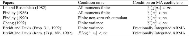
Table 1 gives a summary of the main conditions obtained in the literature for the uniqueness of the MA representation in (1). Apart from such conditions, it is generally also assumed that the spectral density of
Xtis positive almost everywhere.
Note that the condition given by Breidt and Davis (Remark 2, p.386, 1992), as an alternative proof to their Proposition 3.1, is based on the following result:
THEOREM1 (KAGAN ET AL. (1973,P.94)). Letǫjbe a sequence of independent random variables,
and{aj},{bj}be two sequences of real constants such that
i) The sequences{aj/bj:ajbj6= 0}and{bj/aj:ajbj6= 0}are both bounded;
P
ajǫjandPbjǫjconverge a.s. to random variablesUandV respectively;
ii) UandV are independent.
Then, for everyjsuch thatajbj6= 0,ǫjis normally distributed.
In the context of MA processes, this result can be used as follows. Suppose that (3)-(4) hold, where(ǫt)
and(ǫ∗
t)are two i.i.d. processes. Then the variables
ǫ∗t =
∞
X
j=−∞
ajǫt−j and ǫ∗t−h=
∞
X
j=−∞
aj+hǫt−j
are independent. It follows that if the sequences
Table 1.Uniqueness conditions for the non-Gaussian MA representation (1)
Papers Condition onǫt Condition on MA coefficients Lii and Rosenblatt (1982) All moments finite Pj|aj|<∞
Findley (1986) All moments finite Pa2
j<∞ Findley (1990) Finite non-zerorth cumulant Pa2j<∞
Cheng (1992) Finite variance Pa2
j<∞
Breidt and Davis (Prop. 3.1, 1992) Finite variance Fractionally Integrated ARMA Breidt and Davis (Rem. (2) p. 386, 1992) Elog+|ǫt|<∞ Fractionally Integrated ARMA
then either the variablesǫtandǫ∗t are normally distributed, or all theaj’s except one are equal to zero.
The conclusion thus coincides with that of our Proposition 4, but is obtained under (a) less restrictive distributional assumptions on the i.i.d. processes, but (b) more restrictive assumptions on the sequence of coefficients aj. Breidt and Davis (Remark 2, p. 386, 1992) showed that (A1) is satisfied for a MA
polynomial of the formA(z) = Ψ(z)/Φ(z) =P∞
j=0ajzj, whereΨ(z)andΦ(z)are finite-order
polyno-mials under standard assumptions. For more general processes, the boundedness assumption can be very restrictive. For instance, it precludes sequences recursively defined byaj = 0forj≤0andaj=λjaj−1
forj≥1, where(λj)is a sequence converging to zero or to infinity.
APPENDIX2
Proof of Proposition2
In view of (5) withv= 0, we have, for allu∈R,
−σα∗
∗ |u|α∗ =− ∞
X
j=−∞
σα|aj|α|u|α.
Thusα=α∗and, without loss of generality, we can takeσ=σ∗andP∞j=−∞|aj|α= 1. We then have,
by takingv=tuin (5),
∞
X
j=−∞
|aj+taj+h|α= 1 +|t|α, ∀t∈R. (A2)
The right-hand side of this equality is a differentiable function of t except at t= 0. Let us study the differentiability of the left-hand side. Suppose that there existsj0such thataj0 6= 0andaj0+h6= 0. The
functiont7→ |aj0+taj0+h|
αis everywhere differentiable except att
0=−aj0/aj0+h, witht06= 0. The
contribution of all terms of the infinite sum displaying non differentiability att0is
X
j∈J
|aj+taj+h|α=|t−t0|α X
j∈J
|aj+h|α,
whereJ ={j∈Z|aj+t0aj+h= 0}. This contribution must vanish; otherwise, we would have in the
right-hand side of (A2) a function which is differentiable att0 while the left-hand side is not. Hence P
j∈J|aj+h|α= 0, in contradiction with the fact that this sum is bounded below by|aj0+h|
α6= 0.
There-fore, there exists no integerj0such thataj0 6= 0andaj0+h6= 0, which establishes the property.
✷
Proof of Proposition3
By Ibragimov and Linnik (Theorem 2.6.5, 1971), for a variableǫ∗∈DA(α∗), where the limiting stable
distribution has location parameterµ= 0, we have
in the neighborhood of the origin, for some slowly varying functionL∗
1. This equality also holds ifµ6= 0,
the limit law in (6) being uniquely determined up to positive affine transformations. By (5) withv= 0, we thus have
−|u|α∗L∗ 1
1
|u|
=−
∞
X
j=−∞
σα|aj|α|u|α, (A4)
in the neighborhood of 0. Thusα=α∗andL∗1is constant in the neighborhood of 0. It is not restrictive to
assumeσα=L∗
1(1/|u|)in the neighborhood of 0 and P∞
j=−∞|aj|α= 1. We thus are lead to the proof
of Proposition 2.
✷
Proof of Proposition4
By (5) withv= 0and (A3), we have in the neighborhood of 0,
−|u|α∗L∗ 1
1
|u|
=−
∞
X
j=−∞
aj6=0
|aj|α|u|αL1
1
|aju|
. (A5)
i) Let us first show thatα∗=α. Ifα∗< α, the left-hand side term in
|u|α∗−αL∗ 1
1
|u|
=−
∞
X
j=−∞
aj6=0
|aj|αL1 1
|aju|
,
tends to 0 whenu→0, while the right-hand side term does not. We also get a contradiction ifα∗< α,
henceα=α∗.
ii) Now we will show that
L∗1
1
|u|
∼ ∞ X
j=−∞
|aj|α
L1
1
|u|
, whenu→0. (A6)
We will use the next property (see for instance Embrechts, Klüppelberg, Mikosch (1997), Theorem A3.2).
LEMMA1. IfLis a slowly varying function, for anya, b >0, the convergenceL(tx)/L(x)→1when
x→ ∞is uniform on the segment[a, b].
Using Lemma 1 and (A5) withα=α∗we have, in the neighborhood of 0, for some constantsa, b >0to
be chosen later,
L∗ 1 1 |u|
L1
1 |u|
−
∞
X
j=−∞
|aj|α
≤ ∞ X
j=−∞
aj6=0
|aj|α
L1 1 |aju|
L1
1 |u|
−1 ≤ n X
j=−n |aj|α
sup
t∈[a,b] L1 t
|u|
L1
1 |u|
−1 + X
|j|>n aj6=0
|aj|α
L1 1 |aju|
L1
1 |u|
+ X
|j|>n |aj|α
We have, in the neighborhood of 0, forτ=α−s,
S2,n(u) =
X
|j|>n aj6=0
|aj|s|aj|τ
L1 1 |aju|
L1
1 |u|
≤ X
|j|>n aj6=0
|aj|s|aj|τK 1 +|aj|−τ,
which is smaller than an arbitrarily smallς >0fornsufficiently large,n > N say. The same property holds forS3,n. Now let[a, b] =min|j|≤N{|aj|−1, aj 6= 0},max|j|≤N{|aj|−1, aj6= 0}inS1,n(u). We
have
S1,n(u)≤
∞
X
j=−∞
|aj|α
sup
t∈[a,b] L1 t
|u|
L1
1 |u|
−1 ,
which tends to zero using the uniform convergence ofL1.
Thus we have established (A6) and, without generality loss, we can make a scale change on theaj’s to
get, foru6= 0,
L∗1
1
|u|
= ∞ X
j=−∞
|aj|α
L1
1
|u|
. (A7)
iii) Using (A7), Equation (5) can now be written, foru, vin the neighborhood of 0,uv6= 0, as
|u|αL∗1
1
|u|
+|v|αL∗1
1
|v|
=
∞
X
j=−∞
aju+aj+hv6=0
|aju+aj+hv|αL1
1
|aju+aj+hv|
=
∞
X
j=−∞
|aju|αL1 1
|u|
+|aj+hv|αL1 1
|v|
.
Hence, forv=tu,t >0, we get, foruin the neighborhood of 0,
∞
X
j=−∞
aj+taj+h6=0
|aj+taj+h|αL1
1
|aj+taj+h||u|
=
∞
X
j=−∞
|aj|αL1 1
|u|
+|taj+h|αL1 1
t|u|
.
By the same argument as before, using the uniform convergence of the slowly varying functionL1(see
Lemma 1), the asymptotic behavior of these sums in the neighborhood ofu= 0is the same if we replace terms of the formL1
1
x|u|
, withx >0, byL1
1 |u|
. We thus have, for anyt >0,
∞
X
j=−∞
|aj+taj+h|α=
∞
X
j=−∞
(|aj|α+|taj+h|α),
and we are led to the discussion of Proposition 2.
✷
Proof of Proposition5
We use Theorem 2.1 in Kokoszka (1996), which establishes sufficient conditions for two infinite-order lag polynomials whose coefficients may not be absolutely summable to commute. From the assumptions made on the coefficients of the polynomialsa(B) and{a∗(B)}−1, we have ǫ∗
t ={a∗(B)}−1a(B)ǫt,
where the random series{a∗(B)}−1a(B)ǫ
{a∗(B)}−1a(B) =cBℓ for some constantcand some integer ℓ∈Z. Thusa(B) =ca∗(B)Bℓ and the
proof is complete.
✷
Proof of Proposition6
Similarly to (5), we have foru, v∈R,
log|Ψ∗(u)|+ log|Ψ∗(v)|=
K
X
k=1 ∞
X
j=−∞
log|Ψ(uak,j+vak,j+h)|, (A8)
by the independence betweenǫk,tandǫℓ,t′ for any(k, t)6= (ℓ, t′).By the arguments leading to (A4) we
thus have
−|u|α∗L∗ 1
1
|u|
=−
K
X
k=1 ∞
X
j=−∞
σαkk |ak,j|αk|u|αk, (A9)
in the neighborhood of 0. Thusαk=α∗=:αfor allk, andL∗1is constant in the neighborhood of 0,
L∗1 1
|u|
=
K
X
k=1 ∞
X
j=−∞
σαk|ak,j|α.
Now by takingv=tuin the neighborhood ofu= 0, we find that, similarly to (A2),
K
X
k=1 ∞
X
j=−∞
σαk|ak,j+tak,j+h|α= (1 +|t|α) K
X
k=1 ∞
X
j=−∞
σkα|ak,j|α, ∀t∈R. (A10)
Now we can use the following elementary lemma.
LEMMA2. Forα >0, letfγ :t∈R7→fγ(t) =|1 +γt|αand letf∗:t∈R7→f∗(t) =|t|α. LetΓ =
{γi}i∈Ia family of distinct real numbers, withI ⊂Z. The family of functions{f∗, fγ;γ∈Γ}is linearly
independent.
It follows from (A10) and Lemma 2 that for any(k, j)eitherak,jorak,j+his equal to zero. Thus, for any
k, the set{ak,j, j∈Z}reduces to a singleton. The conclusion follows.
✷
Proof of Proposition7
By the independence betweenǫ∗
k,tandǫ∗ℓ,t′ in the one hand, andǫk,tandǫℓ,t′in the other hand, for any (k, t)6= (ℓ, t′), we get from thei-th equation of (13)
K
X
k=1 ∞
X
j=−∞
log|Ψ∗(ua∗i,k,j+va∗i,k,j+h)|,= K
X
k=1 ∞
X
j=−∞
log|Ψ(uai,k,j+vai,k,j+h)|.
Thus, by arguments already used,
K
X
k=1 ∞
X
j=−∞
(σ∗
k)α
∗
k|a∗ i,k,j|α
∗
k|u|α∗k= K
X
k=1 ∞
X
j=−∞
σkαk|ai,k,j|αk|u|αk,
in the neighborhood of 0. It follows that{αk;k= 1, . . . , K}={αk∗;k= 1, . . . , K}and thusα1=α∗1<
. . . < αK =α∗K and
P∞
j=−∞(σk∗)αk|a∗i,k,j|α
∗
k|u|α∗k=P∞ j=−∞σ
αk
k |ai,k,j|αk|u|αk for k= 1, . . . , K. It
is thus not restrictive to assume σk =σk∗and
P∞
j=−∞|a∗i,k,j|α
∗
k|u|α∗k =P∞
similarly to (A10),
K
X
k=1 ∞
X
j=−∞
(σk∗)αk|ai,k,j∗ +ta∗i,k,j+h|αk = K
X
k=1 ∞
X
j=−∞
σαk
k |ai,k,j+tai,k,j+h|
αk, ∀t∈ R,
which, using the fact that the powersαkare different, entails, fork= 1, . . . , K,
∞
X
j=−∞
|a∗i,k,j+ta∗i,k,j+h|αk =
∞
X
j=−∞
|ai,k,j+tai,k,j+h|αk, ∀t∈R. (A11)
Let (ηt) be an i.i.d. sequence of symmetric αk- stable distributed random variables,
ηt∼ S(αk,0,1,0). The left hand side of (A11) characterizes the distribution of the
process (a∗
i,k(B)ηt). It follows that a∗i,k(B)ηt d
= 1
σkai,k(B)ǫk,t. Therefore, we have
ηt=d σ1 k{a
∗
i,k(B)}−1ai,k(B)ǫk,tand we can conclude as in the proof of Proposition 5.
✷
REFERENCES
Breidt, F.J. and R.A., Davis (1992) Time-reversibility, identifiability and independence of innovations for stationary time-series.Journal of Time Series Analysis13, 377–390.
Brockwell, P., and R., Davis (1991)Time Series : Theory and Methods. Springer Verlag, New-York.
Chan, K.-S., Ho, L.-H. and H. Tong A note on time-reversibility of multivariate linear processes.
Biometrika93, 221–227.
Cheng, Q. (1992) On the unique representation of non-Gaussian linear processes.Annals of Statistics20,
1143–1145.
Cheng, Q. (1999) On time-reversibility of linear processes.Biometrika86, 483–486.
Cline, D.B.H. (1983) Infinite series of random variables with regularly varying tails. Unpublished docu-ment, The University of British Columbia.
Embrechts, P., Klüppelberg, C. and T. Mikosch (1997)Modelling extremal events.Springer.
Findley, D. (1986) The uniqueness of moving average representation with independent and identically distributed random variables for non-Gaussian stationary time series.Biometrika73, 520–521.
Findley, D. (1990) Amendments and corrections: The uniqueness of moving average representation with independent and identically distributed random variables for non-Gaussian stationary time series.
Biometrika77, 235.
Gouriéroux, G. and J-M. Zakoian (2013) Explosive Bubble Modelling by Noncausal Process. CREST Discussion Paper 2013-04.
Hallin, M., Lefèvre, C. and M. Puri (1988) On time-reversibility and the uniqueness of moving average representations for non-Gaussian stationary time series.Biometrika75, 170–171.
Ibragimov, I.A. and Yu. V. Linnik (1971) Independent and stationary sequences of random variables.
Wolters-Noordoff, Groningen.
Kagan, A., Linnik, Yu. V. and C. Rao (1973)Characterization problems in mathematical statistics,
Wi-ley: New-York.
Kokoszka, P. S. (1996) Prediction of infinite variance fractional ARIMA.Probability and Mathematical statistics16, 65–83.
Lii, K.S. and M. Rosenblatt (1982) Deconvolution and estimation of transfer function phase and coeffi-cients for non-Gaussian linear processes.Annals of Statistics10, 1195–1208.
Rosenblatt, M. (2000) Gaussian and non-Gaussian linear time series and random fields. Springer–
Verlag, New York.
Samorodnitsky G. and M. S. Taqqu (1994)Stable Non-Gaussian Random Processes, Chapman & Hall,