Quantifying sentence complexity based on eye-tracking measures
Abhinav Deep Singh, Poojan Mehta, Samar Husain, Rajakrishnan Rajkumar
Indian Institute of Technology Delhi New Delhi, India
{abhinav1010.ads, poojanmehta8994}@gmail.com {samar, raja}@hss.iitd.ac.in
Abstract
Eye-tracking reading times have been attested to reflect cognitive processes underlying sentence comprehension. However, the use of reading times in NLP applications is an underexplored area of research. In this initial work we build an automatic system to assess sentence complexity using automatically predicted eye-tracking reading time measures and demonstrate the efficacy of these reading times for a well known NLP task, namely, readability assessment.
We use a machine learning model and a set of features known to be significant predictors of reading times in order to learn per-word reading times from a corpus of English text having reading times of human readers. Subsequently, we use the model to predict reading times for novel text in the context of the aforementioned task. A model based only on reading times gave competitive results compared to the systems that use extensive syntactic features to compute linguistic complexity. Our work, to the best of our knowledge, is the first study to show that
automatically predictedreading times can successfully model the difficulty of a text and can be deployed in practical text processing applications.
1 Introduction
Quantifying the complexity of a sentence has been one of the central goals of psycholinguistics (Gibson, 2000; Lewis, 1996; Levy, 2008). Decades of experimental research has shown us that certain kinds of syntactic patterns are more complex than others. For example, in English, object relative clause is generally assumed to be more difficult than the active counterpart e.g. (Gibson, 2000). Similarly center-embeddings lead to more complexity (Lewis and Vasishth, 2005). Such experiments try to establish a causal link between complex linguistic pattern and processing difficulty. The difficulty is manifested in slower response of a measurable variable (e.g. reaction time, gaze duration, etc.). The eye-tracking experimental paradigm is known to capture processing difficulty during naturalistic reading (Just and Carpenter, 1980; Frazier and Rayner, 1982; Clifton et al., 2007).
Deploying insights from eye-movement research for Natural Language Processing (NLP) tasks is an upcoming area of research. Previous works have used fixation durations (and saccades) as features in their prediction models. For example, eye-movement data has been used to model translation difficulty (Mishra et al., 2013), sentiment annotation complexity (Joshi et al., 2014), and sarcasm detection (Mishra et al., 2016). Recent works have also incorporated eye-tracking data as features in sequence models for part-of-speech tagging (Barrett et al., 2016; Barrett and Søgaard, 2015).
In this exploratory work, we build an automatic system to assess sentence complexity using auto-matically predicted eye-tracking reading time measures and demonstrate the efficacy of these reading times for READABILITY ASSESSMENT.Readability assessmentis the task of automatically classifying text into different levels of difficulty (Petersen and Ostendorf, 2009; Feng, 2010; Vajjala and Meurers, 2014). One use of such difficulty assessment could be to evaluate text simplification, e.g. to automati-cally simplify Wikipedia text for the English L2 learners (Zhu et al., 2010; Woodsend and Lapata, 2011; Coster and Kauchak, 2011; Wubben et al., 2012; Siddharthan and Mandya, 2014). There is also a large This work is licenced under a Creative Commons Attribution 4.0 International Licence. Licence details: http:// creativecommons.org/licenses/by/4.0/
body of work that has attempted to quantify and automatically compute the complexity of a text using various linguistic features (Kincaid et al., 1975; Flesch, 1948; Gunning, 1968; Si and Callan, 2001). See Vajjala Balakrishna (2015) for an extensive review. Such quantification becomes necessary for tasks such as text simplification (Siddharthan, 2014) and for L2 learners’ systems (Schwarm and Ostendorf, 2005). So far previous work in text simplification (and more generally in NLP) has not explored directly using various eye-tracking reading time measures while quantifying linguistic complexity. Clearly, such reading times are not available for new text and hence need to be automatically predicted. For machine translation evaluation, Mishra et al. (2013) formulate a translation difficulty index which is computed using eye-movement data, but they do not directly predict reading time measures.
Our work, to the best of our knowledge, is the first study to show that automatically predicted reading times can successfully model the difficulty of a text and can be deployed in practical text processing applications. We use a machine learning model and a set of features known to be significant predictors of reading times in order to learn per-word reading times from a corpus of English text having reading times of human readers. Subsequently, we use the model to predict reading times for novel text for readability assessment. For this task, a model based only on reading times gave competitive results compared to the systems that use extensive syntactic features. Our best-performing model, which combines learned read-ing times with other sentence-level features, comes close to state-of-the-art results reported previously for the dataset used in this work (Ambati et al., 2016; Vajjala and Meurers, 2016).
The paper is organized as follows. Section 2 provides an overview of our two-level hierarchical sys-tem. Section 3 describes our model to automatically predict per-word reading time using a wide range of lexical as well as syntactic features. Subsequently, Section 4 reports on our readability assessment experiments using predicted reading times from the above model. Finally, we conclude the paper in Section 5.
2 Approach
Our approach comprises of two modules:
1. Reading time (RT) prediction: System-1 using lexical and syntactic features to predict the reading times (RTs) of each word in the sentence
2. Sentence level prediction: System-2 using predicted reading times (outputted by System-1) and other sentence-level features for the task of readability assessment.
Supervised learning algorithms were employed to train both systems (1) and (2).
2.1 Motivation: Why predict RTs?
An obvious question that could be asked about our approach is ‘Why build a two-step system?’ or ‘Why use predicted RTs when one can use linguistic features directly?’. Several reasons present themselves in support of our approach:
1. We would like to explore the extent to which behavioural measure of processing difficulty can be used to predict sentential complexity.
2. It is known from the experimental psycholinguistic literature that eye-tracking RTs can reflect in-creased linguistic complexity (Clifton et al., 2007; Vasishth et al., 2012). A model that predicts RTs for each word in a sentence can contribute to a fine-grained picture of reading difficulty at various points in a sentence, in contrast to sentence-level features.
3 System 1 - Predicting Reading Times
In this section we discuss the features that can impact reading time prediction. We do this using an abla-tion study and using Pearson’s coefficient. Only those features which cause an increase in R2goodness score are selected for the final model.
3.1 Data Set
The Dundee eye-tracking corpus (Kennedy, 2003) was used to train the reading time prediction system. It has eye-movement record of 10 participants on a large collection of newspaper text. We used 2378 sentences (50597 words) from the Dundee corpus. We randomly divided the data (at sentence level, and not word level) into training (60%), development (20%) and test (20%) splits. RTs for all the subjects were pooled into one set.1
Our task is to predict the reading times of each word in a sentence. We will focus on 4 types of measures – first fixation duration, first pass duration, regression path duration and total duration. Together these measures represent the ‘early’ and ‘late’ measures and are known to reflect sentence processing difficulty (Clifton et al., 2007). First fixation duration (FFD) is the duration of the first fixation on a region. First pass duration(FPD) is the sum of all the fixations on a region from the time it was first entered until it was left. Regression path duration(RPD) is the sum of all the fixations on a region from the time it was first entered until moving to the right of the region. Total fixation duration (TD) of a region is the sum of all fixations on a region including re-fixations after it was left. All these measures, of course, assume that the region in question has been fixated.
3.2 Feature Set
The features used in the model have been attested to influence lexical and syntactic processing reading and it has been established conclusively that all these features are significant predictors of reading times (Rayner, 1998; Juhasz and Rayner, 2003; Demberg and Keller, 2008; Clifton et al., 2007; van Schijndel and Schuler, 2015). We use both low level predictors like word length, sentence length, word frequency and age of acquisition (in years) as well as high level predictors like surprisal.
Word lengthhas been taken as it is from the Dundee corpus. Sentence lengthis the number of words in a sentence. Word frequency is the unigram frequency in the entire English Wikipedia text. Theage of acquisitiongives the average age and standard deviation at which a word is learnt (Kuperman et al., 2012). This reflects the familiarity of a word, which has been shown to affect lexical processing (Juhasz and Rayner, 2006). These features have previously been shown to be helpful in predicting the difficulty in reading (Vajjala Balakrishna, 2015). British National Corpus (BNC) (Aston and Burnard, 1998) was used to calculate forward transition probability– P(wk|wk−1) andbackward transition probability – P(wk|wk+1)for each word.
In addition, we also addedsurprisal(Hale, 2001; Levy, 2008), entropy reduction(Hale, 2006), em-bedding depth and embedding difference (Wu et al., 2010) computed by an incremental probabilistic left-corner parser (van Schijndel et al., 2013). Surprisalmodels comprehension difficulty where words which are more predictable in a given syntactic or lexical context are read faster (lower surprisal values) compared to less predictable words (higher surprisal values). Mathematically, surprisal at word k+1, Sk+1 = −logP(wk+1|w1...wk). In our incremental left-corner probabilistic parser, strings of a
lan-guage are assumed to be generated by Probabilistic Context Free Grammars (PCFGs). So each wordwk
has a prefix probability computed by summing the probabilities of all trees T in the span of words w1 to wk. Surprisal is estimated as the difference in the prefix probabilities at successive words. Both syntactic
and lexical surprisal are standout predictive measures for reading times regardless of word class (Wu et al., 2010).
Entropy reductionat word index =iis defined as:max{0, Hi−Hi−1}, whereHiis the entropy
func-tion. So, it is the reduction in (syntactic) uncertainty at the appearance of word at index =i. Embedding depthis a quantitative measure reflecting memory load caused due to center embeddings (left branching parse tree nodes contained within right branching ones). A weighted version of this measure obtained
by multiplying with the parse probability is also used.Embedding differenceis defined as the difference between the embedding depth at the current beam and the previous beam (Wu et al., 2010). (Howcroft, 2015) also uses the features from Wu et al (2010) for readability assessment and shows that they induce modest gains over other features. However, that work does not use reading times as features. In addition, we added eight more features emitted by the left-corner parser. These represent hierarchical structure decisions made by the parser and encode memory operations like cue activation, initiation, termination and wait. For more details, please refer to (van Schijndel and Schuler, 2013).
3.3 Model
We used linear regression using python-sklearn (Pedregosa et al., 2011) to predict the reading times. All features were standardized.
3.4 Experiments
Pearson’s Coefficients Study
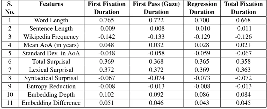
We calculated Pearson’s coefficient for each of the features w.r.t. the four reading times, first fixation duration, first pass duration, regression path duration, andtotal fixation duration. Almost all correla-tions reported are significant at p<0.01.2. These results can be seen in Table 1. We find that most of the
features show low correlation with the 4 duration measures in question (first fixation, first pass, regres-sion and total fixation duration). However, as expected the word length and surprisals is found to have high positive correlation while frequency and familiarity (mean age of acquisition - AoA) have negative correlations with RT. We move forward with the ablation study with first fixation duration, as among the four durations features seem to be most correlated with first fixation in general.
S. Features First Fixation First Pass (Gaze) Regression Total Fixation
No. Duration Duration Duration Duration
1 Word Length 0.765 0.722 0.700 0.668
2 Sentence Length -0.009 -0.008 -0.010 -0.011
3 Wikipedia Frequency -0.142 -0.133 -0.129 -0.126
4 Mean AoA (in years) 0.048 0.032 0.028 0.021
5 Standard Dev. in AoA -0.048 -0.058 -0.059 -0.067
6 Total Surprisal 0.369 0.368 0.365 0.358
7 Lexical Surprisal 0.372 0.372 0.369 0.363
8 Syntactical Surprisal -0.067 -0.074 -0.073 -0.072
9 Entropy Reduction -0.008 -0.013 -0.008 -0.013
10 Embedding Depth 0.102 0.092 0.086 0.084
[image:4.595.73.523.370.554.2]11 Embedding Difference 0.051 0.046 0.043 0.045
Table 1: Pearson’s Correlation Coefficient of features w.r.t. different reading times.
Ablation Study
We did an ablation study to select the best features for the model that predicts first fixation duration. The results can be seen in Table 2. In total there were 20 features in the model. Instead of exploring all (20!) orders, features were added incrementally based on the following rationale. At first, we added all the low-level predictors of reading times described in previous work (Demberg and Keller, 2008). In the case of the remaining features, we added the frequency-based predictors of reading difficulty next and finally memory-based predictors. This distinction was based on Collin Phillips’ theory of ground-ing (Phillips, 2013), which characterizes memory load costs as predictors of comprehension difficulty after frequency-based costs have already been taken into account. If the goodness of the learned regres-sion curve improved, the feature was retained in the final model3. The process helped in ascertaining the
2Except in case of sentence length w.r.t. first fixation and first pass, where p-value is 0.03 and 0.02 respectively.
3Issues related to multicollinearity have also been sidestepped in this initial analysis. We intend to address these issues in
relevance of individual feature in the model. We find that the word frequency, age of acquisition, total and syntactic surprisals lead to largest increase in the goodness score. Interestingly, lexical surprisal does not appear to be a significant contributor, probably because, word frequency already captures much of the effect (cf. Demberg and Keller, 2008).
S.No. Features R2score S.No. Features R2score
1 Word Length 0.267 7 Lexical Surprisal 0.575
2 Sentence Length 0.500 8 Syntactical Surprisal 0.579
3 Word Frequency 0.504 9 Entropy Reduction 0.579
4 Mean Age of Acquisition (AoA) 0.532 10 Embedding Depth 0.580
5 Standard Deviation in AoA 0.533 11 Embedding Difference 0.580
[image:5.595.73.533.129.228.2]6 Total Surprisal 0.576 12 Hierarchical structure feats 0.585
Table 2: Ablation study done on features by adding them incrementally to the FFD regression model.
Implementation and Results
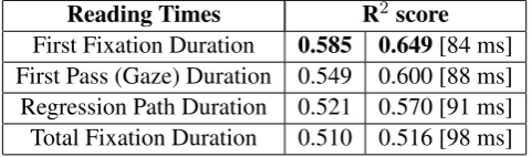
We trained our model for all the four reading times, i.e. RTs for all the subjects were pooled into one set. The results can be seen in Table 3. R2score gives the goodness of the model. A closer look at the predicted reading times showed that on a number of occasions the regression model predicted very low non-zero reading times which were non-existent in the Dundee corpus. Therefore, we set a threshold (84 ms) for predicted reading times (for Fixed Fixation Duration), and any prediction less than this threshold was reduced to 0.0 ms. The threshold was fixed on the development set. As can be seen from table 3, using a threshold led to an improvement.
Reading Times R2 score First Fixation Duration 0.585 0.649[84 ms] First Pass (Gaze) Duration 0.549 0.600 [88 ms] Regression Path Duration 0.521 0.570 [91 ms] Total Fixation Duration 0.510 0.516 [98 ms]
Table 3: Performance of System 1 on different eye-tracking measures. The number inside [] shows the threshold value.
3.5 Discussion
Predictions for first fixation duration are consistently better than other eye-tracking measures. The post hoc addition of threshold improved the performance significantly, and we see that R2 score reaches upto 0.649 for first-fixation duration. First-fixation durations are known to reflect both low-level lexical processing (Clifton et al., 2007) as well as syntactic processes (Vasishth et al., 2012).
We were unable to do equally well on other measures such as first pass duration, regression path duration and total fixation duration compared to first fixation duration. So, while the current results are promising, more experiments with regards to alternative models need to be explored. In particular, it will be interesting to investigate if feature selection differs from one eye-movement to the other. This will shed some light on the feature-measure mapping. In addition, alternative/additional features that could correlate better with these measures need to be tried out. Finally, other measures such as regression probability, etc. need to investigated. These issues will be taken up as part of future work.
4 System 2 - Readability Assessment
The task that we evaluate the system discussed in the previous section is readability assessment. The exact task of readability assessment is the following:
[image:5.595.179.420.390.461.2]Vajjala and Meurers (2016) have previously built a system to accomplish this task using various lin-guistic features. They used features produced by a non-incremental syntactic parser and found them to be useful in the task. They also used lexical semantic properties from WordNet, features encod-ing morphosyntactic properties of lemmas, word-level psycholencod-inguistic features such as concreteness, meaningfulness and imageability extracted from the MRC psycholinguistic database as well as age of acquisition (AoA). Their model achieved an accuracy of 74.58%.
Motivated by the incremental nature of human sentence processing, Ambati et al. (2016) use features extracted from an incremental Combinatory Categorical Grammar (CCG) parser to achieve higher ac-curacy on this task. Their feature set included sentence length, height of the CCG derivation, the final number of constituents, CCG rule counts and complexity of CCG category. Their model achieved an accuracy of 78.87%.
Our system is also motivated by human sentence processing. However, unlike Ambati et al. (2016), we directly use predicted reading times to model complexity of a sentence. As discussed in section 3, the model that predicts reading times is based on psycholinguistically motivated lexical and syntactic features.
4.1 Data Set
The dataset used for evaluation is the dataset released by Ambati et al. (2016). This is a cleaned subset of the parallel sentence pairs collected by Hwang et al. (2015). The data contains 150K sentence pairs of standard Wikipedia (WIKI) and simple Wikipedia (SIMPLEWIKI). Ambati et al. (2016) further removed pairs containing identical sentences which resulted in 117K clean pairs. We randomly divided the data into training (60%), development (20%) and test (20%) splits.
4.2 Feature Set
Sentence-1 features Sentence-2 features
sentence1 word1: 169 sentence2 word1: 189
sentence1 word2: 110 sentence2 word2: 309
sentence1 word3: 215 sentence2 word3: 85
sentence1 word4: 219 sentence2 word4: 85
... ...
[image:6.595.187.412.404.555.2]... ...
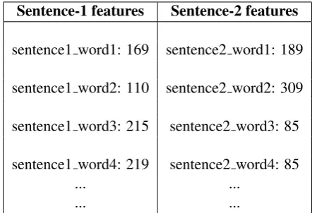
Table 4: Example features in a sentence pair (each column contains the feature name and value separated by a space). The features values are in milliseconds.
Vajjala and Meurers (2016) formulated the readability assessment task as a ranking task, instead of a classification task. In our model we simply classify within a pair of sentences. For a sentence, we first predict reading time for each word (using System 1). The features are of the form “Word Posi-tion:Predicted RT”. “Word Position” is the feature name and corresponds to the position of a word in a sentence, and predicted RT (which models first fixation duration) is its value. We define a sample as a pair of sentences. To avoid using same feature name for each sentence we simply concatenate “sen-tence1” or “sentence2” before all the feature names. For example, consider the following sentence pair from the dataset:
1. With a higher humidity, the rate of evaporation is less.
Assuming the following reading times for words in the first sentence – “with: 169ms”, “a: 110ms”, “higher: 215ms”, “humidity: 219ms”, “the: 149ms” and so on, the features for our ‘Base RT’ model are depicted in Table 4. The features from both the sentences together are then used to train the classification system. So the total number of features equal to twice the number of words in the longest sentence in our corpus as we work with sentence pairs.
The ‘Base RT’ model uses only these word-level features. We also experimented with a model that uses sentence-level features in addition to the base model features. This ‘Extended RT’ model contained the following additional features: sentence length, normalized (w.r.t. sentence length) sum of predicted reading time of the sentence. The incremental probabilistic left-corner parser (van Schijndel et al., 2013) was used to further add the following features: sum of total surprisal of all words, sum of lexical surprisal of all words, sum of syntactical surprisal of all words and log of parse probability of the entire sentence.
4.3 Model
As discussed in section 4.2, the pair of sentences are represented as a multiset of its features. We use a bag of words unigram model, except the features we use are not just words the sentences have, but ‘wordposition:predicted RT’. The model assumes that relevant properties of the syntactic structure have already been captured by System-1 (discussed in section 3) to predict the reading time. Logistic regres-sion classifier, using python-sklearn (Pedregosa et al., 2011) was used for the classification task. We also experimented with SVM (Hearst et al., 1998) and SVMrank (Joachims, 2006), used by Vajjala and
Meurers (2016), but these models were unable to outperform the logistic regression model.4
4.4 Results
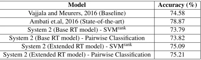
A 10 fold cross-validation was done to obtain the accuracies. We evaluated the model with all four predicted durations (first fixation, first pass, regression and total). The best results were obtained with predicted first fixation duration therefore we show only those figures in Table 5.
Model Accuracy (%)
Vajjala and Meurers, 2016 (Baseline) 74.58
Ambati et.al, 2016 (State-of-the-art) 78.87
System 2 (Base RT model) - SVMrank 73.79
System 2 (Base RT model) - Pairwise Classification 73.82
System 2 (Extended RT model) - SVMrank 75.09
[image:7.595.132.467.414.515.2]System 2 (Extended RT model) - Pairwise Classification 75.21
Table 5: Performance of models with predicted first fixation duration.
Table 5 depicts 74.58% as the classification accuracy of Vajjala and Meurers (2016). It needs to be noted that the Vajjala and Meurers (2016) paper reports an accuracy of 82.7% on their evaluation data. The number 74.58% is taken from the Ambati et. al (2016) paper. This figure was obtained by Ambati and colleagues as a result of running the Vajjala and Meurers code on their evaluation data5. As
mentioned before, we used the same evaluation data as Ambati et. al (2016). Hence Table 5 results are all based on the same dataset and thus directly comparable.
4.5 Discussion
We tested our model with the both SVMrank strategy as used by Vajjala and Meurers (2016) and the
pairwise classification strategy discussed in section 4.2. In both cases, pairwise classification performs slightly better than SVMrank.
The Base RT model using just the predicted reading times and the word positions achieves an accuracy of 73.82%. This shows that predicted reading time alone can be successfully employed as a predictor
4Time taken by the system - Incremental Parser: The data set was divided into 100 sections and parsing was done in parallel.
Each section took almost 10 hours. Final training: Takes around 5 min for around 120K sentences pairs.
to compute sentence complexity. Our Extended RT model achieves an accuracy of 75.21% which is marginally better than the Vajjala and Meurers (2016) model. The Ambati et al. (2016) system is still the best performing system. To see how much do reading times contribute to our system, we ran a model with just sentence level features from extended model and no Base RT features, which had the accuracy of 73.6% (1.6 points lower). This indicates that reading times do contribute to boost our model accuracy. Note that, similar to Ambati et al. (2016), our RT prediction model (discussed in section 3) uses many syntactic features. These features include surprisal, entropy reduction, embedding depth, embedding difference, etc. The syntactic features in the Ambati et al. (2016) model (such as CCG rule counts, CCG categories) are much more fine-grained in terms of the different syntactic phenomenon that they capture. In would be very interesting to see if these fine-grained features can lead to improvement in a model that predicts eye-movement reading measures. We plan to test this out as part of our future work. Also, our results are based on just one eye-tracking measure, i.e. first fixation duration. Future work can try to improve this performance by exploring multiple measures in a single model.
5 Conclusion
We used a machine learning model and a set of features known to be significant predictors of reading times in order to learn per-word reading times from a corpus of English text having reading times of human readers. Subsequently, we used the model to predict reading times for novel text in the context ofreadability assessment. For this task, a model based only on reading times gave competitive results compared to the systems that use extensive syntactic features.
Notwithstanding the debate on strict vs loose connection between parsing processes and eye move-ments (Just and Carpenter, 1980) (also see, Vasishth et al., 2012), it has been conclusively established that sentence parsing events are manifested in reading times. Since automatic quantification of complex-ity is required in a number of NLP tasks/evaluations, models based on automatically predicted reading times present themselves as an attractive alternatives to the current methods. Our work, to the best of our knowledge, is the first study to show that such a model is indeed viable. We demonstrated that it can be used to successfully model the difficulty of a text and can be deployed in practical text processing applications. In addition to technological advances in field of NLP, we also envisage that our system can potentially facilitate scientific inquiries in human sentence processing. Prior to running behavioural experiments involving human subjects, our method can be used to formulate precise hypothesis by gen-erating reading times for the test sentences.
Acknowledgement
We thank the three anonymous reviewers for their insightful comments. Their feedback has helped us improve the paper. Any errors that remain are our own.
References
Bharat Ram Ambati, Siva Reddy, and Mark Steedman. 2016. Assessing relative sentence complexity using an incremental CCG parser. InProceedings of the North American Chapter of the Association for Computational Linguistics on Language technologies, California, USA.
Guy Aston and Lou Burnard. 1998. The BNC handbook: exploring the British National Corpus with SARA. Capstone.
Maria Barrett and Anders Søgaard. 2015. Reading behavior predicts syntactic categories. InProceedings of the Nineteenth Conference on Computational Natural Language Learning, pages 345–349, Beijing, China, July. Association for Computational Linguistics.
C. Clifton, A. Staub, and K. Rayner. 2007. Eye movements in reading words and sentences. In R. Van Gompel, M. Fisher, W. Murray, and R. L. Hill, editors, Eye movements: A window on mind and brain, chapter 15. Elsevier.
William Coster and David Kauchak. 2011. Simple English Wikipedia: a new text simplification task. In Proceed-ings of the 49th Annual Meeting of the Association for Computational Linguistics: Human Language Technolo-gies.
Vera Demberg and Frank Keller. 2008. Data from eye-tracking corpora as evidence for theories of syntactic processing complexity. Cognition, 109(2):193–210.
Lijun Feng. 2010.Automatic readability assessment. City University of New York. R. Flesch. 1948. A new readability yardstick.Journal of Applied Psychology, 32(3):221.
L. Frazier and K. Rayner. 1982. Making and correcting errors during sentence comprehension: Eye movements in the analysis of structurally ambiguous sentences.Cogn Psychol, 14:178–210.
Edward Gibson. 2000. The dependency locality theory: A distance-based theory of linguistic complexity. Image, language, brain, pages 95–126.
R. Gunning. 1968. The Technique of Clear Writing. McGraw-Hill Book Company, 2nd ed.
John Hale. 2001. A probabilistic Earley parser as a psycholinguistic model. InProceedings of the second meeting of the NAACL, pages 1–8. Association for Computational Linguistics.
John Hale. 2006. Uncertainty about the rest of the sentence. Cognitive Science, 30:643–672.
Marti A. Hearst, Susan T Dumais, Edgar Osman, John Platt, and Bernhard Scholkopf. 1998. Support vector machines. IEEE Intelligent Systems and their Applications, 13(4):18–28.
David Howcroft. 2015. Ranking sentences by complexity. Master’s thesis, Saarland University.
William Hwang, Hannaneh Hajishirzi, Mari Ostendorf, and Wei Wu. 2015. Aligning sentences from standard wikipedia to simple wikipedia. InProceedings of the 2015 Conference of the North American Chapter of the Association for Computational Linguistics (NAACL).
Thorsten Joachims. 2006. Training linear SVMs in linear time. In Proceedings of the 12th ACM SIGKDD international conference on Knowledge Discovery and Data Mining, pages 217–226. ACM.
Aditya Joshi, Abhijit Mishra, Nivvedan Senthamilselvan, and Pushpak Bhattacharyya. 2014. Measuring sentiment annotation complexity of text. InProceedings of the 52nd ACL, pages 36–41, June.
Barbara J Juhasz and Keith Rayner. 2003. Investigating the effects of a set of intercorrelated variables on eye fixa-tion durafixa-tions in reading. Journal of Experimental Psychology: Learning, Memory, and Cognition, 29(6):1312. Barbara J Juhasz and Keith Rayner. 2006. The role of age of acquisition and word frequency in reading: Evidence
from eye fixation durations. Visual Cognition, 13(7-8):846–863.
Marcel Adam Just and Patricia A. Carpenter. 1980. A theory of reading: from eye fixations to comprehension.
Psychological Review, 87:329–354.
Alan Kennedy and Jo¨el Pynte. 2005. Parafoveal-on-foveal effects in normal reading.Vision research, 45(2):153– 168.
A Kennedy. 2003. The Dundee Corpus [CD-ROM]. Psychology Department, University of Dundee.
J. Peter Kincaid, Lieutenant Robert P. Jr. Fishburne, Richard L. Rogers, and Brad S. Chissom. 1975. Derivation of new readability formulas (Automated Readability Index, Fog Count and Flesch Reading Ease Formula) for navy enlisted personnel.
Victor Kuperman, Hans Stadthagen-Gonzalez, and Marc Brysbaert. 2012. Age-of-acquisition ratings for 30,000 English words.Behavior Research Methods, 44(4):978–990.
Roger Levy. 2008. Expectation-based syntactic comprehension.Cognition, 106(3):1126 – 1177.
R. L. Lewis. 1996. Interference in short-term memory: The magical number two (or three) in sentence processing.
Journal of Psycholinguistic Research, 25(1):93–116.
Abhijit Mishra, Pushpak Bhattacharyya, and Michael Carl. 2013. Automatically predicting sentence translation difficulty. InProceedings of the 51st ACL, pages 346–351, August.
Abhijit Mishra, Diptesh Kanojia, and Pushpak Bhattacharyya. 2016. Predicting readers’ sarcasm understandability by modeling gaze behavior. InProceedings of the Thirtieth AAAI Conference on Artificial Intelligence, Phoenix, Arizona, USA., pages 3747–3753.
F. Pedregosa, G. Varoquaux, A. Gramfort, V. Michel, B. Thirion, O. Grisel, M. Blondel, P. Prettenhofer, R. Weiss, V. Dubourg, J. Vanderplas, A. Passos, D. Cournapeau, M. Brucher, M. Perrot, and E. Duchesnay. 2011. Scikit-learn: Machine learning in Python. Journal of Machine Learning Research, 12:2825–2830.
Sarah E Petersen and Mari Ostendorf. 2009. A machine learning approach to reading level assessment. Computer Speech & Language, 23(1):89–106.
Colin Phillips. 2013. Some arguments and non-arguments for reductionist accounts of syntactic phenomena.
Language and Cognitive Processes, 28:156–187.
Keith Rayner. 1998. Eye movements in reading and information processing: 20 years of research. Psychological Bulletin, 124(3):372.
S. Schwarm and M. Ostendorf. 2005. Reading level assessment using support vector machines and statistical language models. InProceedings of the 43rd Annual Meeting of the Association for Computational Linguistics. L. Si and J. Callan. 2001. A statistical model for scientific readability. InProceedings of the 10th International
Conference on Information and Knowledge Management (CIKM), pages 574–576.
Advaith Siddharthan and Angrosh Mandya. 2014. Hybrid text simplification using synchronous dependency grammars with hand-written and automatically harvested rules. InEACL, pages 722–731.
A. Siddharthan. 2014. A survey of research on text simplification. International Journal of Applied Linguistics: Special issue on Recent Advances in Automatic Readability Assessment and Text Simplification, 165(2):259– 298.
Sowmya Vajjala and Detmar Meurers. 2014. Assessing the relative reading level of sentence pairs for text simpli-fication. InEACL, pages 288–297.
Sowmya Vajjala and Detmar Meurers. 2016. Readability-based sentence ranking for evaluating text simplification.
arXiv preprint arXiv:1603.06009.
Sowmya Vajjala Balakrishna. 2015. Analyzing Text Complexity and Text Simplification: Connecting Linguistics, Processing and Educational Applications. Ph.D. thesis, Universit¨at T¨ubingen.
Marten van Schijndel and William Schuler. 2013. An analysis of frequency- and memory-based processing costs. In Proceedings of the 2013 Conference of the North American Chapter of the Association for Computational Linguistics: Human Language Technologies, pages 95–105, Atlanta, Georgia, June. Association for Computa-tional Linguistics.
Marten van Schijndel and William Schuler. 2015. Hierarchic syntax improves reading time prediction. In Pro-ceedings of the 2015 Conference of the North American Chapter of the Association for Computational Lin-guistics: Human Language Technologies, pages 1597–1605, Denver, Colorado, May–June. Association for Computational Linguistics.
Marten van Schijndel, Andy Exley, and William Schuler. 2013. A model of language processing as hierarchic sequential prediction.Topics in Cognitive Science, 5(3):522–540.
Shravan Vasishth, Titus von der Malsburg, and Felix Engelmann. 2012. What eye movements can tell us about sentence comprehension. Wiley Interdisciplinary Reviews: Cognitive Science, pages 125–134.
Kristian Woodsend and Mirella Lapata. 2011. WikiSimple: Automatic simplification of wikipedia articles. In
AAAI.