S. Fr¨oschle, F.D. Valencia (Eds.): Workshop on Expressiveness in Concurrency 2010 (EXPRESS’10). EPTCS 41, 2010, pp. 31–45, doi:10.4204/EPTCS.41.3
c
A, Cerone & M. Hennessy This work is licensed under the Creative Commons Attribution License.
(Extended Abstract)
Andrea Cerone Trinity College Dublin
Dublin, Ireland
School of Computer Science and Statistics∗ [email protected]
Matthew Hennessy Trinity College Dublin
Dublin, Ireland
School of Computer Science and Statistics [email protected]
Process behaviour is often defined either in terms of the tests they satisfy, or in terms of the logical properties they enjoy. Here we compare these two approaches, using extensional testing in the style of DeNicola, Hennessy, and a recursive version of the property logic HML.
We first characterise subsets of this property logic which can be captured by tests. Then we show that those subsets of the property logic capture precisely the power of tests.
1
Introduction
One central concern of concurrency theory is to determine whether two processes exhibit the same be-haviour; to this end, many notions of behavioural equivalence have been investigated [Gla93]. One ap-proach, proposed in [DH84], is based on tests. Intuitively two processes are testing equivalent, p≈testq,
relative to a set of tests T if p and q pass exactly the same set of tests from T . Much here depends of course on details, such as the nature of tests, how they are applied and how they succeed.
In the framework set up in [DH84] observers have very limited ability to manipulate the processes under test; informally processes are conceived as completely independent entities who may or may not react to testing requests; more importantly the application of a test to a process simply consists of a run to completion of the process in a test harness. Because processes are in general nondeterministic, formally this leads to two testing based equivalences, p≈mayq and p≈mustq; the latter is determined by the set
of tests a process guarantees to pass, written p must satisfy t, while the former by those it is possible to pass, p may satisfy t. The may equivalence provides a basis for the so-called trace theory of processes [Hoa85] , while the must equivalence can be used to justify the various denotational models based on
Failures used in the theory of CSP, [Hoa85, Old87, DN83].
Another approach to behavioural equivalence is to say that two processes are equivalent unless there is a property which one enjoys and the other does not. Here again much depends on the chosen set of properties, and what it means for a process to enjoy a property. Hennessy Milner Logic [HM85] is a modal logic often used for expressing process properties in term of the actions they are able to perform. It is well-known that it can be used, via differing interpretations, to determine numerous variations on
bisimulation equivalence, [Mil89, AILS07]. What has received very little attention in the literature
however is the relationship between these properties and tests. This is the subject of the current paper. More specifically, we address the question of determining which formulae of a recursive version of the Hennessy Milner Logic, which we will refer to as recHML, can be used to characterise tests. This problem has already been solved in [AI99] for a non-standard notion of testing; this is discussed
more fully later in the paper. But we will focus on the more standard notions of may and must testing mentioned above.
To explain our results, at least intuitively, let us introduce some informal notation; formal definitions will be given later in the paper. Suppose we have a propertyφand a test t such that:
for every process p, p satisfiesφif and only if p may satisfy the test t.
Then we say the formulaφmay-represents the test t. We use similar notation with respect to must testing.
Our first result shows that the power of tests can be captured by properties; for every test t
(i) There is a formulaφmay(t) which may-represents t; see Theorem 5.2
(ii) There is a formulaφmust(t) which must-represents t; see Theorem 4.18
Properties, or at least those expressed in recHML, are more discriminating than tests, and so one would not expect the converse to hold. But we can give simple descriptions of subsets of recHML, called
mayHML and mustHML respectively, with the following properties:
(a) Everyφ∈mayHML may-represents some test tmay(φ); see Theorem 5.1 (b) Everyφ∈mustHML must-represents some test tmust(φ); see Theorem 4.14
Moreover because the formulaeφmay(t), φmust(t) given in (i), (ii) above are in mayHML, mustHML re-spectively, these sub-languages of recHML have a pleasing completeness property. For example letφbe any formula from recHML which can be represented by some test t with respect to must testing; that is
p satisfiesφif and only if p must satisfy t. Then, up to logical equivalence, the formulaφis guaranteed to be already in the sub-language mustHML; that is, there is a formulaψ∈mustHML which is logically
equivalent toφ. The language mayHML has a similar completeness property for may testing.
We now give a brief overview of the remainder of the paper. In the next section we recall the formal definitions required to state our results precisely. Our results in the may case will only hold when the set of tests we consider come from a finite state finite branching LTS. Further, we also require for the LTS of processes to be finite branching when dealing with the must testing relation. The reader should also be warned that we use a slightly non-standard interpretation of recHML.
We then explain both may and must testing, where we take as processes the set of states from an arbitrary LTS, and give an explicit syntax for tests. In Section 3 we give a precise statement of our results, including definitions of the sub-languages mayHML and mustHML, together with some illuminating examples. The proofs of these results for the must case are given in Section 4, while those for the may case are outlined in Section 5. We end with a brief comparison with related work.
2
Background
One formal model for describing the behaviour of a concurrent system is given by Labelled Transition
Systems (LTSs):
Definition 2.1. A LTS over a set of actions Act is a tripleL=hS, Actτ, −→iwhere: • S is a countable set of states
• Actτ=Act∪ {τ}is a countable set of actions, whereτdoes not occur in Act • −→⊆S×Actτ×S is a transition relation.
We use a,b,· · · to range over the set of external actions Act, andα, β,· · · to range over Actτ. The standard
notation s−→α s′will be used in lieu of (s, α,s′)∈−→. States of a LTSLwill also be referred to as (term)
Let us recall some standard notation associated with LTSs. We write s−→α if there exists some s′such that s−→α s′, s−→if there existsα∈Actτsuch that s
α
−→, and s−→α/ , s−→/ for their respective negations. We use Succ(α,s) to denote the set{s′|s−→α s′}, and Succ(s) forS
α∈ActτSucc(α,s). If Succ(s) is finite for
every state s∈S the LTS is said to be finite branching. Finally, a state s diverges, denoted s⇑, if there is an infinite path of internal moves s−→τ s′−→ · · ·τ , while it converges, s⇓, otherwise.
For a given LTS, each action of the form−→a can be interpreted as an observable activity; informally speaking, this means that each component which is external to the modeled system can detect that such an action has been performed. On the other hand, the actionτis meant to represent internal unobservable activity; this gives rise to the standard notation for weak actions. s=⇒τ s′ Is used to denote reflexive transitive closure of−→, while sτ =⇒a s′denotes s=⇒τ s′′−→a s′′′=⇒τ s′. When s=α⇒s′we say that s′is an
α-derivative of s. The associated notation s=α⇒, s=⇒, s=α⇒/ and s=⇒/ have the obvious definitions. It is common to define many operators on LTSs for interpreting process algebras. In this paper we will use only one, a parallel operator designed with testing in mind.
Definition 2.2 (Parallel composition).
LetL1=hS1,Act1τ,−→i,L2=hS2, Act2τ,−→ibe LTSs. The parallel composition ofL1andL2is a LTS
L1|L2= hS1×S2, {τ},−→i, where−→is defined by the following SOS rules:
s−→τ s′
s|t−→τ s′|t
t−→τ t′
s|t−→τ s|t′
s−→a s′ t−→a t′
s|t−→τ s′|t′
s|t is used as a conventional notation for (s,t).
The first two rules express the possibility for each component of a LTS to perform independently an internal activity, which cannot be detected by the other component. The last rule models the synchro-nization of two processes executing the same action; this will result in unobservable activity.
2.1 Recursive HML
Hennessy Milner Logic (HML), [HM85] has proven to be a very expressive property language for states
in an LTS. It is based on a minimal set of modalities to capture the actions a process can perform, and what the effects of performing such actions are. Here we use a variant in which the interpretation depends on the weak actions of an LTS.
Definition 2.3 (Syntax of recHML). Let Var be a countable set of variables. The language recHML is defined as the set of closed formulae generated by the following grammar:
φ ::= tt | ff | X | Acc(A) | φ1∨φ2 | φ1∧φ2 | hαiφ | [α]φ | min(X, φ) | max(X, φ)
Here X is chosen from the countable set of variables Var. The operators min(X, φ),
max(X, φ) act as binders for variables and we have the standard notions of free and bound variables, and
associated binding sensitive substitution of formulae for variables.
Let us recall the informal meaning of recHML operators. A formula of the formhαiφexpresses the need for a process to have anα-derivative which satisfies formulaφ, while formula [α]φexpresses the need for allα-derivatives (if any) of a converging process to satisfy formulaφ.
~ttρ , S ~ffρ , ∅
~Xρ , ρ(X) ~Acc(A)ρ , {s|s⇓, if s=⇒τ s′then∃a∈A.s′=⇒}a
~hαiφρ , h·α·i(~φρ) ~[α]φρ , [·α·](~φρ)
~φ1∨φ2ρ , ~φ1ρ∪~φ2ρ ~φ1∧φ2ρ , ~φ1ρ∩~φ2ρ
~min(X, φ)ρ , T
{P|~φρ[X7→P]⊆P} ~max(X, φ)ρ , S
[image:4.612.90.533.78.156.2]{P|P⊆~φρ[X7→P]}
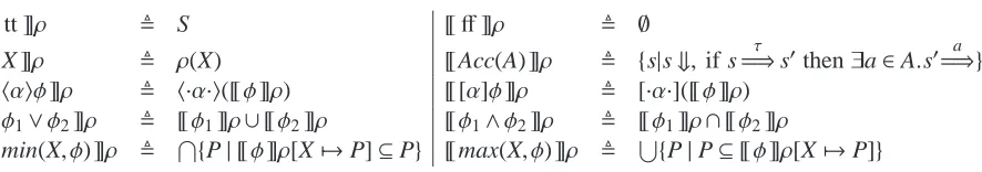
Table 1: Interpretation of recHML
processes for which eachτ-derivative has at least an a-derivative for a∈Act. min(X, φ) and max(X, φ) allow the description of recursive properties, respectively being the least and largest solution of the equation X=φover the powerset domain of the state space.
Formally, given a LTShS,Actτ,−→i, we interpret each (closed) formula as a subset of 2S. The set 2s is a complete lattice and the semantics is determined by interpreting each operator in the language as a monotonic operator over this complete lattice. The binary operators∨,∧are interpreted as set theoretic union and intersection respectively while the unary operators are interpreted as follows:
h·α·iP={s|s=⇒α s′for some s′∈P} [·α·]P={s|s⇓, and s=α⇒s′implies s′∈P}
where P ranges over subsets of 2S.
Open formulae in recHML can be interpreted by specifying, for each variable X, the set of states for which the atomic formula X is satisfied. Such a mappingρ: Var→2S is called environment. Let Env be the set of environments. A formulaφof recHML will be interpreted as a function ~φ: Env→2S. We will use the standard notation ρ[X7→P] to refer to the environment ρ′ such that ρ′(X)=P and
ρ′(Y)=ρ(Y) for all variables Y such that X,Y.
The definition of the interpretation ~·is given in Table 2.1. When referring to the interpretation of a closed formulaφ∈recHML, we will omit the environment application, and sometimes use the standard
notation p|=φfor p∈~φ.
Our version of HML is non-standard, as we have added a convergence requirement for the inter-pretation of the box operator [α]. The intuition here is that, as in the failures model of CSP [Hoa85], divergence represents underdefinedness. So if a process does not converge all of its capabilities have not yet been determined; therefore one can not quantify over all of itsαderivatives, as the totality of this set has not yet been determined. Further, the operator Acc(A) is also non-standard. It has been introduced for the sake of simplicity, as it will be useful later; in fact it does not add any expressive power to the logic, since for each finite set A⊆Act the formula Acc(A) is logically equivalent to [τ](W
a∈Ahaitt ). As usual, we will writeφ{ψ/X}to denote the formulaφwhere all the free occurrences of the variable
X are replaced withψ. We will use the congruence symbol≡for syntactic equivalence.
The language recHML can be extended conservatively by adding simultaneous fixpoints, leading to the language recHML+. Given a sequence of variables (X) of length n>0, and a sequence of formulaeφ
of the same length, we allow the formula mini(X, φ) for 1≤i≤n. This formula will be interpreted as the i-th projection of the simultaneous fixpoint formula.
vari-ables and formulae of length n.
~min(X, φ)ρ , \{P|~φiρ[X7→P]⊆Pi∀1≤i≤n}
~mini(X, φ)ρ , πi(~min(X, φ)ρ)
whereπiis the i-th projection operator, and intersection over vectors of sets is defined pointwise. Again we will omit the environment application if a formula of the form mini(X, φ) is closed, that is the only variables that occur in φare those in X. Intuitively, an interpretation ~min(X, φ), where
X=hX1,· · ·,Xniandφ=hφ1,· · ·, φni, is the least solution (over the set of vectors of length n over 2S) of the equation system given by Xi=φifor all i=1,· · ·,n, while~mini(X, φ)is the i-th projection of such a vector. Simultaneous fixpoints do not add any expressivity to recHML, as shown below:
Theorem 2.5 (Bek´ıc, [Win93]).
For each formulaφ∈recHML+there is a formulaψ∈recHML such that~φ=~ψ.
Later we will need the following properties of simultaneous fixpoints:
Theorem 2.6 (Fixpoint properties).
(i) Let (P) be a vector of sets from 2S satisfying ~φiρ[X7→ P]⊆ Pi for every 1 ≤i≤ n. Then
~mini(X, φ)ρ⊆Pi
(ii) Letρminbe an environments such thatρmin(Xi)=~mini(X, φ).Then~mini(X, φ)=~φiρmin.
2.2 Tests
Another way to analyse the behaviour of a process is given by testing. Testing a process can be thought of as an experiment in which another process, called test, detects the actions performed by the tested process, reacting to it by allowing or forbidding the execution of a subset of observables. After observing the behaviour of the process, the test could decree that it satisfies some property for which the test was designed for by reporting the success of the experiment, through the execution of a special actionω.
Formally speaking, a test is a state from a LTST =hT,Actωτ,−→i, where Actωτ =Actτ∪ {ω}andωis an action not contained in Actτ.
Given a LTS of processesL=hS,Actτ,−→i, an experiment consists of a pair p|t from the product LTS (L | T). We refer to a maximal path p|t−→τ p1|t1−→τ . . . .−→τ pk|tk
τ
−→. . .as a computation of p|t.
It may be finite or infinite; it is successful if there exists some n≥0 such that tn ω
−→. As onlyτ-actions can be performed in an experiment, we will omit the symbolτin computations and in computation prefixes. Successful computations lead to the definition of two well known testing relations, [DH84]:
Definition 2.7 (May Satisfy, Must Satisfy). Assuming a LTS of processes and a LTS of tests, let s and t be a state and a test from such LTSs, respectively. We say
(a) s may satisfy t if there exists a successful computation for the experiment s|t.
(b) s must satisfy t if each computation of the experiment s|t is successful.
Later in the paper we will use a specific LTS of tests, whose states are all the closed terms generated by the grammar
Again in this language X is bound in µX.t, and the test t{t′/X} denotes the test t in which each free occurrence of X is replaced by t′. The transition relation is defined by the following rules:1
α.t−→α t
t1
α −→t′1
t1+t2
α −→t1′
t2
α −→t′2
t1+t2
α
−→t2′ µX.T
τ
−→t{(µX.t)/X}
The last rule states that a test of the formµX.t can always perform aτ-action before evolving in the test t{µX.t/X}. This treatment of recursive processes will allow us to prove properties of paths of recursive tests and experiments by performing an induction on their length. Further, the following properties hold for a test t in grammar (1):
Proposition 2.8. LetT =hT,Actτ,−→ibe the LTS generated by a state t in grammar (1): thenT is both
branching finite and finite state.
3
Testing formulae
Relative to a process LTShS,Actτ,−→iand a test LTShT,Actτω,−→i, we now explore the relationship between tests from our default LTS of tests and formulae of recHML. Given a test t, our goal is to find a formulaφsuch that the set of processes which may satisfy/must satisfy such a test is completely
characterised by the interpretation ~φ. Moreover, we aim to establish exactly the subsets of recHML for which each formula can be checked by some test, both in the may and must case.
For this purpose some definitions are necessary:
Definition 3.1. Letφbe a recHML formula and t a test. We say that:
• φmust-represents the test t, if for all p∈S , p must satisfy t if and only if p|=φ.
• φis must-testable whenever there exists a test whichφmust-represents.
• t is must-representable, if there exists someφ∈recHML which must-represents it respectively.
Similar definitions are given for may testing.
First some examples.
Example 3.2 (Negative results).
(a) φ=[a]ff is not may-testable.
Let s∈~[a]ff; a new process p can be built starting from s by letting p−→τ p, whenever s−→α s′ then p−→α s′.
Processes p and s may satisfy the same set of tests. However, p< ~[a]ff, as p⇑. Therefore no test may-represents [a]ff.
(b) φ=haitt is not must-testable.
We show by contradiction that there exists no test t that must-representsφ. To this end, we perform a case analysis on the structure of t.
• t−→ω : Consider the process 0 with no transitions. Then 0 must satisfy t, whereas 0< ~φ.
• t−→ω/ : Let s∈~φand consider the process p built up from s according to the rules of the example above; we have p∈~φ. On the other hand, p must satisfy t is not true; indeed the experiment p|t leads to the unsuccessful computation p|tp|t· · ·.
1For the sake of clarity, the rules use an abuse of notation, by consideringαas an action from Act
Therefore there is no test t which must-representsφ. (c) φ=haitt∧ hbitt is not may-testable.
Let s be the process whose only transitions are s−→a 0, s−→b 0. Let also p,p′be the processes whose only transitions are p−→a 0, p′−→b 0. We have s∈~φ, whereas p,p′< ~φ. We show that whenever s may satisfy a test t, then either p may satisfy t or p′may satisfy t. Thus there exists no test which
is may-satisfied by exactly those processes in~φ, and thereforeφis not may-representable. First, notice that if s may satisfy t, then at least one of the following holds:
(i) t=ω⇒,
(ii) t=⇒a t′=ω⇒,
(iii) t=⇒b t′=ω⇒.
If t=ω⇒, then trivially both p and p′ may satisfy t. On the other hand, if t=⇒a t′=ω⇒, then there exist t′′,tω such that t
τ
=⇒t′′−→a t′=⇒τ tω ω
−→. We can build the computation fragment for p | t such that
p | t· · ·p | t′′0 | t′· · ·0 | tω
which is successful. Hence p may satisfy t. Finally, The case t=⇒b t′=ω⇒is similar.
(d) In an analogous way to (c) it can be shown that [a]ff∨[b]ff is not must-testable.
We now investigate precisely which formulae in recHML can be represented by tests. To this end, we define two sub-languages, namely mayHML and mustHML.
Definition 3.3. (Representable formulae)
• The language mayHML is defined to be the set of closed formulae generated by the following
recHML grammar fragment:
φ ::= tt | ff | X | hαiφ | φ1∨φ2 | min(X, φ) (2)
• The language mustHML is defined to be the set of closed formulae generated by the following
recHML grammar fragment:
φ ::= tt | ff | Acc(A) | X | [α]φ | φ1∧φ2 | min(X, φ) (3)
Note that both sub-languages use the minimal fixpoint operator only; this is not surprising, as informally at least testing is an inductive rather than a coinductive property. Since there exist formulae of the form [α]φ, φ1∧φ2which are not may-representable, the [·] modality and the conjunction operator, have not
been included in mayHML The same argument applies to the modalityh·iand the disjunction operator∨ in the must case, which are therefore not included in mustHML.
Note also that the modality [·] is only used in mustHML, which will be compared with must-testing. No diverging process must satisfy a non-trivial test t, i.e. such that t−→ω/ . Hence, in this setting, the convergence restriction on this modality is natural.
4
The must case
We will now develop the mathematical basis needed to relate mustHML formulae and the must testing relation; in this section we will assume that the LTS of processes is branching finite.
Lemma 4.1. Letφ∈mustHML, and let p∈~φ, where p⇑: then~φis the entire process space, i.e.
~φ=S .
This lemma has important consequences; it means formulae in mustHML either have the trivial interpre-tation as the full set of states S , or they are only satisfied by convergent states.
Definition 4.2. LetCbe the set of subsets of S determined by:
• S ∈ C,
• X∈ C,s∈X implies s⇓.
Proposition 4.3. Cordered by set inclusion is a continuous partial order, cpo.
Proof. The empty set is obviously the least element inC. So it is sufficient to show that if X0⊆X1⊆ · · ·
is a chain of elements inCthenS
nXnis also inC.
We can now take advantage of the fact that mustHML actually has a continuous interpretation in (C,⊆). The only non trivial case here is the continuity of the operator [·α·]:
Proposition 4.4. Suppose the LTS of processes is finite-branching: If X0⊆X1⊆ · · · is a chain of elements inCthen
[
n
[·α·]Xn=[·α·] [
n
Xn.
This continuous interpretation of mustHML allows us to use chains of finite approximations for these formulae of mustHML. That is givenφ∈mustHML and k≥0, recursion free formulaeφkwill be defined such that~φk⊆~φ(k+1)and S
k≥0=~φ. We can therefore reason inductively on approximations in
order to prove properties of recursive formulae.
Definition 4.5 (Formulae approximations). For each formulaφin mustHML define
φ0 , ff
φ(k+1) , φ ifφ= tt,ffor Acc(A)
([α]φ)(k+1) , [α](φ)(k+1) (φ1∧φ2)(k+1) , φ(k1+1)∧φ(k2+1)
(min(X, φ))(k+1) , (φ{min(X, φ)/X})k
It is obvious that for everyφ∈mustHML,~φk⊆~φ(k+1)for every k≥0; The fact that the union of the approximations ofφconverges toφitself depends on the continuity of the interpretation:
Proposition 4.6.
[
k≥0
Proof. This is true in the initial continuous interpretation of the language, and therefore also in our
interpretation. For details see [CN78].
Having established these properties of the interpretation of formulae in mustHML, we now show that they are all must-testable. The required tests are defined by induction on the structure of the formulae.
Definition 4.7. For eachφin mustHML define tmust(φ) as follows:
tmust( tt ) = ω.0 (4)
tmust(ff) = 0 (5)
tmust(Acc(A)) = X
a∈A
a.ω.0 (6)
tmust(X) = X (7)
tmust([τ]φ) = τ.tmust(φ) (8)
tmust([a]φ) = a.tmust(φ)+τ.ω.0 (9)
tmust(φ1∧φ2) =
ω.0 ifφ1∧φ2is closed and
logically equivalent to tt
τ.T mustφ1+τ.tmust(φ2) otherwise
(10)
tmust(min(X, φ)) =
tmust(φ) ifφis closed
µX.tmust(φ) otherwise (11)
For each formulaφin mustHML, the test tmust(φ) is defined in a way such that the set of processes
which must satisfy tmust(φ) is exactly~φ. Before supplying the details of a formal proof of this
state-ment, let us comment on the definition of tmust(φ).
Cases (4), (5) and (7) are straightforward. In the case of Acc(A), the test allows only those action which are in A to be performed by a process, after which it reports success.
For the box operator, a distinction has to be made between [a]φand [τ]φ. In the former we have to take into account that a converging process which cannot perform a weak a-action satisfies such a property; thus, synchronisation through the execution of a a-action is allowed, but a possibility for the test to re-port success after the execution of an internal action is given. In the case of [τ]φ no synchronization with any action is required; however, since we are adding a convergence requirement to formulaφ, we have to avoid the possibility that the test tmust([τ]φ) can immediately perform aωaction. This is done by
requiring the test tmust([τ]φ) to perform only an internal action.
Finally, (10) and (11) are defined by distinguishing between two cases; this is because a formula of the formφ1∧φ2or min(X, φ) can be logically equivalent to tt , whose interpretation is the entire state space.
However, the second clause in the definition of tmust(φ) for such formulae require the test to perform aτ
action before performing any other activity, thus at most converging processes must satisfy such a test. In order to give a formal proof that tmust(φ) does indeed capture the formulaφwe need to establish
some preliminary properties. The first essentially says that no formula of the form min(X, φ), withφnot closed, will be interpreted in the whole state space.
Lemma 4.9.
• p must satisfyµX.t implies p must satisfy t{µX.t/X}.
• p⇓,p must satisfy t{µX.t/X}implies p must satisfyµX.t.
Note that the premise p⇓is essential in the second part of this lemma, asµX.t cannot perform aω
action; therefore it can be must-satisfied only by processes which converge.
Proposition 4.10. Suppose the LTS of processes is finitely branching. If p must satisfy tmust(φ) then
p∈~φ.
Proof. Suppose p must satisfy tmust(φ); As both the LTS of processes (by assumption) and the LTS of tests (Proposition 2.8) are finite branching, the maximal length of a successful computation |p,t|is defined and finite. This is a direct consequence of Konig’s Lemma [BJ89]. Thus it is possible to perform an induction over|p,tmust(φ)|to prove that p∈~φk. The result will then follow from Proposition 4.6.
• If|p,tmust(φ)|=0 then tmust(φ)
ω
−→, and hence for each p∈S p must satisfy tmust(φ). Further it is
not difficult to show thatφis logically equivalent to tt , hence p∈~φ.
• If |p,tmust(φ)|=n+1 then the validity of the Theorem follows from an application of an inner
induction onφ. We show only the most interesting case, which is φ=min(X, ψ). There are two possible cases.
(a) If X is not free inψthen the result follows by the inner induction, as min(X, ψ) is logically equivalent toψ, and tmust(min(X, ψ))≡tmust(ψ) by definition.
(b) If X is free inψthen, by Lemma 4.9 p must satisfy tmust(ψ){µX.tmust(ψ)/X}, which is
syntac-tically equal to tmust(ψ{min(X, ψ)/X}).
Since|p,tmust(ψ{min(X, ψ)/X})|<|p,tmust(φ)|, by inductive hypothesis we have
p∈~ψ{min(X, ψ)/X}kfor some k, hence p∈~φ(k+1).
To prove the converse of Proposition 4.10 we use the following concept:
Definition 4.11 (Satisfaction Relation). Let R⊆S×mustHML and for anyφlet (Rφ)={s | s Rφ}. Then R is a satisfaction relation if it satisfies
(R tt ) = S
(Rff) = ∅
(R Acc(A)) = {s|s⇓,s=⇒τ s′implies S (s′)∩A,∅ } (R [α]φ) ⊆ [·α·](Rφ)
(Rφ1∧φ2) ⊆ (Rφ1)∩(Rφ2)
(Rφ{min(X, φ)/X}) ⊆ (R min(X, φ))
Satisfaction relations are defined to agree with the interpretation ~·. Indeed, all implications re-quired for satisfaction relations are satisfied by |=. Further, as ~min(X, φ) is defined to be the least solution to the recursive equation X=φ, we expect it to be the smallest satisfaction relation.
Proposition 4.12. The relation|=is a satisfaction relation. Further, it is the smallest satisfaction relation.
Proposition 4.12 ensures that, for any satisfaction relation R,|= is included in R; in other words, if
p|=φthen p Rφ. Next we consider the relation Rmustsuch that p Rmustφwhenever p must satisfy tmust(φ),
Proposition 4.13. The relation Rmustis a satisfaction relation.
Proof. We proceed by induction on formulaφ. Again, we only check the most interesting case. Supposeφ=min(X, ψ). We have to show p must satisfy tmust(ψ{φ/X}) implies p must satisfy tmust(φ).
We distinguish two cases:
(a) X does not appear free inψ. then tmust(φ)=tmust(ψ), andψ{φ/X}=ψ. This case is trivial.
(b) X does appear free inφ: in this case tmust(φ)=µX.tmust(ψ), and tmust(ψ{φ/X}) has the form
tmust(ψ){µX.tmust(ψ)/X}. By Lemma 4.8~φ ,S ; therefore Lemma 4.1 ensures that p⇓, and hence
by Lemma 4.9 it follows p must satisfy tmust(φ).
Combining all these results we now obtain our result on the testability of mustHML.
Theorem 4.14. Suppose the LTS of processes is finite-branching. Then for everyφ∈mustHML, there exists a test tmust(φ) such thatφmust-represents the test tmust(φ).
Proof. We have to show that for any process p, p must satisfy tmust(φ) if and only if p∈~φ. One direction follows from Proposition 4.10. Conversely suppose p∈~φ. By Proposition 4.12 it follows that for all satisfaction relations R it holds p Rφ; hence, by Proposition 4.13, p Rmustφ, or equivalently
p must satisfy tmust(φ).
We now turn our attention to the second result, namely that every test t is must-representable by some formula in mustHML. Let us for the moment assume a branching finite LTS of tests in which the state space T is finite.
Definition 4.15. Assume we have a test-indexed set of variables{Xt}. For each test t∈T define ϕt as
below:
ϕt , tt if t−→ω (12)
ϕt , ff if t−→/ (13)
ϕt , ( ^ a,t′:t−→a t′
[a]Xt′) ∧Acc({a|t
a
−→}) if t−→ω/ ,t−→τ/ ,t−→ (14)
ϕt , ( ^
t′:t−→τ t′
[τ]Xt′) ∧ (
^
a,t′:t−→a t′
[a]Xt′) if t−→ω/ ,t−→τ (15)
Takeφtto be the extended formula mint(XT, ϕT), using the simultaneous least fixed points introduced
in Section 2.1.
Notice that we have a finite set of variables{Xt}and that the conjunctions in Definition 4.15 are finite, as the LTS of tests is finite state and finite branching. These two conditions are needed forφt to be well defined.
Formulaφt captures the properties required by a process to must satisfy test t. The first two clauses of the definition are straightforward. If t cannot make an internal action or cannot report a success, but can perform a visible action a to evolve in t′, then a process should be able to perform a=⇒a transition and evolve in a process p′such that p′must satisfy t′. The requirement Acc({a | t−→}) is needed becausea a synchronisation between the process p and the test t is required for p must satisfy t to be true.
will perform a transition t−→τ t′ after p has executed an arbitrary number of internal actions. Thus, we require that for each transition p=⇒τ p′, p′must satisfy t′.
We now supply the formal details which lead to state that formula φt characterises the test t. Our immediate aim is to show that the two environments, defined by
ρmin(Xt),~φt ρmust(Xt),{p | p must satisfy t}
are identical. This is achieved in the following two propositions.
Proposition 4.16. For all t∈T it holds thatρmin(Xt)⊆ρmust(Xt).
Proof. We just need to show that~ϕtρmust⊆ρmust(Xt): the result follows from an application of the
minimal fixpoint property, Theorem 2.6 (i). The proof is carried out by performing a case analysis on t.
We will only consider Case (14), as cases (12) and (13) are trivial and Case (15) is handled similarly. Assume p∈~ϕtρmust. We have
(a) p⇓,
(b) whenever p=⇒τ p′there exists an action a∈Act such that t−→a and p′=a⇒,
(c) whenever p=⇒a p′and t−→a t′, p′∈ρmust(Xt′), i.e. p′must satisfy t′.
Conditions (a) and (b) are met since p∈~Acc({a|t−→)a and t−→a for some a∈Act, while (c) is true
because of p∈~V
a,t′: t−→a t′[a]Xt′.
To prove that p∈ρmust(Xt) we have to show that every computation of p|t is successful. To this end,
consider an arbitrary computation of p|t; condition (b) ensures that such a computation cannot have the
finite form
p | tp1 | t· · ·pk | tpk+1 | t· · ·pn | t (16)
For such a computation we have that pn τ
=⇒p′, and there exists p′′ with p′−→a p′′ for some action a and test t′such that t−→a t′. Therefore we have a computation prefix of the form
p | tp1 | t· · ·pn | t· · ·p′ | tp′′ | t′,
hence the maximality of computation (16) does not hold.
Further, condition (a) ensures that a computation of p | t cannot have the form
p | tp1 | t· · ·pk | tpk+1 | t· · ·
Therefore all computations of p | t have the form
p | tp1 | t· · ·pn | tp′ | t′
with p′must satisfy t′by condition (c); then for each computation of p | t there exist p′′,t′′such that
p | t· · ·p′ | t′· · ·p′′ | t′′,
and t′′−→. Hence, every computation from pω | t is successful.
Proof. We have to show p must satisfy t implies p∈~φt.
Suppose p must satisfy t; since we are assuming that the set T , as well as the set S , contains only finite branching tests (processes), the maximal length of a successful computation fragment|p,t|is defined and finite.
Therefore we proceed by induction on|p,t|; the main technical property used is the Fixpoint Property 2.6(ii).
• k=0: In this case, t−→, and hence for all pω ∈S we have p must satisfy t. Moreover,ϕt= tt , and hence for all p∈S p∈~φtρmin,
• k>0. There are several cases to consider, according to the structure of the test t: 1. t−→ω/ ,t−→τ/ ,t−→: we first show that p∈~Acc({a|t−→)a ρmin.
Since p must satisfy t, we have p⇓. Consider a computation fragment of the form
p | t· · ·pn | t
As p⇓, we require that all computations rooted in pn | t will eventually contain a term of the
form pk | t′, where t′,t. Further, as t−→τ/ , such a test should follow from a synchronisation between pk−1 and t. We have that then that, whenever p=⇒τ pn, there exists an action a such that t−→a t′ and pn=⇒a pk, which combined with the constraint p⇓ is equivalent to
p∈~Acc({a|t−→)a .
We also have to show that p∈~[a]Xt′ρmin. Let p
a
−→p′. Then p must satisfy t implies
p′ must satisfy t′. Moreover, we have |p′,t′|< k. By inductive hypothesis, we have that p′∈~φt′, that is p′∈ρmin(Xt′). Then the result p∈~[a]Xt′ρminholds.
2. t−→ω/ ,t−→τ : A similar analysis as in the case above can be carried out.
Combining these two propositions we get our second result. Let us say that a test t from a LTS of tests T =hT,Actτω,→iis finitary if the derived LTS consisting of all states inT accessible from t is finite.
Theorem 4.18. Assuming the LTS of processes is finite branching, every finitary test t is
must-representable.
Proof. Consider any test t. We can apply Definition 4.15 to the finite LTS of tests reachable from t to
obtain a formulaφtwhich must-represents test t. Notice that this formula is not contained in recHML, as it uses simultaneous least fixpoints. However, by Theorem 2.5 there exists a formulaφmust(t)∈recHML
such that~φt=~φmust(t), thus t is must-representable. Further, since each operator used in Definition 4.15 to defineϕtbelongs to mustHML, it is ensured thatφmust(t)∈mustHML. As a Corollary we are able to show that mustHML is actually the largest language (up to logical equivalence) of must-testable formulae.
Corollary 4.19. Supposeφis a formula in recHML which is must-testable. Then there exists someψin mustHML which is logically equivalent to it.
Proof. Suppose φis must-testable. By theorem 4.14 there exists a finite test t=tmust(φ) which must-representsφ. Further, by theorem 4.18 there exists a formulaψ=φmust(t)∈mustHML which must-tests
for t. Therefore
p∈~φ⇔p must satisfy tmust(φ)⇔p∈~ψ
5
The may case
In this paper we simply state the corresponding theorems for may testing:
Theorem 5.1. Suppose the LTS of processes is finite branching. Then for everyφ∈mayHML, there exists a test tmay(φ) such that,φmay-represents the test tmay(φ).
Theorem 5.2. Assuming the LTS of processes is finite branching, every test t is may-representable.
Corollary 5.3. Suppose φis a formula in recHML which is may-testable. Then there exist someψin mayHML which is logically equivalent to it.
Proof. Similar to that of Corollary 4.19.
Our proofs for Theorem 5.2 and Theorem 5.1 are similar in style to the corresponding results for
must testing, namely, namely Theorem 4.18 and Theorem 4.14. Also , as we point out in the Conclusion,
they can be recovered by dualising the proofs of the corresponding Theorems in [AI99].
6
Conclusions
We have investigated the relationship between properties of processes as expressed in a recursive version of Hennessy-Milner logic, recHML, and extensional tests as defined in [DH84]. In particular we have shown that both may and must tests can be captured in the logic, and we have isolated logically complete sub-languages of recHML which can be captured by may testing and must testing. One consequence of these results is that the may and must testing preorders of [DH84] are determined by the logical properties in these sub-languages mayHML and mustHML respectively; however this is already a well-known result, [Hen85].
However these results come at the price of modifying the satisfaction relation; to satisfy a box for-mula a process is required to converge. One consequence of this change is that the language recHML no longer characterises the standard notion of weak bisimulation equivalence, as this equivalence is insen-sitive to divergence. But there are variations on bisimulation equivalence which do take divergence into account; see for example [Wal88, HP80].
The research reported here was initiated after reading [AI99]; there a notion of testing was used which is different from both may and must testing. They define s passes the test t whenever no computation from
s|t can perform the success actionω, and give a sub-language which characterises this form of testing. It is easy to check that s passes t if and only if, in our terminology, s may t is not true. So their notion of testing is dual to may testing, and therefore, not surprisingly, our results on may testing are simply dual versions of theirs. However we believe our results on must testing, specifically Theorem 4.14 and Theorem 4.18, are new.
We have concentrated on properties associated essentialy with the behavioural theory based on ex-tensional testing. However there are a large number of other behavioural theories; see [Gla93] for an extensive survey, including their characterisation in terms of observational properties.
References
[AI99] Luca Aceto and Anna Ing ´olfsd ´ottir. Testing hennessy-milner logic with recursion. In Thomas [Tho99], pages 41–55.
[AILS07] Luca Aceto, Anna Ing ´olfsd ´ottir, Kim Guldstrand Larsen, and Jiri Srba. Reactive Systems: Modelling, Specification and Verification. Cambridge University Press, New York, NY, USA, 2007.
[BJ89] George S. Boolos and Richard C. Jeffrey. Computability and Logic. Cambridge University Press, third edition, 1989.
[BRR87] W. Brauer, W. Reisig, and G. Rozenberg, editors. Petri Nets: Applications and Relationships to Other Models of Concurrency. Number 255 in Lecture Notes in Computer Science. Springer-Verlag, 1987.
[CN78] Bruno Courcelle and Maurice Nivat. The algebraic semantics of recursive program schemes. In Winkowski [Win78], pages 16–30.
[DH84] R. DeNicola and M. Hennessy. Testing equivalences for processes. Theoretical Computer Science, 24:83–113, 1984.
[DN83] Rocco De Nicola. A Complete Set of Axioms for a Theory of Communicating Sequential Processes. In FCT, pages 115–126, 1983.
[Gla93] Rob J. van Glabbeek. The linear time - branching time spectrum ii. In CONCUR ’93: Proceedings of the 4th International Conference on Concurrency Theory, pages 66–81, London, UK, 1993. Springer-Verlag.
[Hen85] M. Hennessy. Acceptance trees. Journal of the ACM, 32(4):896–928, October 1985.
[HM85] Matthew Hennessy and Robin Milner. Algebraic laws for nondeterminism and concurrency. J. ACM, 32(1):137–161, 1985.
[Hoa85] C.A.R. Hoare. Communicating Sequential Processes. Prentice-Hall, 1985.
[HP80] Matthew C. B. Hennessy and Gordon D. Plotkin. A term model for CCS. In Mathematical Founda-tions of Computer Science 1980, Proceedings of the 9th Symposium, volume 88 of Lecture Notes in Computer Science, pages 261–274, Rydzyna, Poland, 1–5 September 1980. Springer.
[Mil89] R. Milner. Communication and Concurrency. Prentice-Hall, 1989.
[NV07] Sumit Nain and Moshe Y. Vardi. Branching vs. linear time: Semantical perspective. In Namjoshi et al. [NYHO07], pages 19–34.
[NYHO07] Kedar S. Namjoshi, Tomohiro Yoneda, Teruo Higashino, and Yoshio Okamura, editors. Automated Technology for Verification and Analysis, 5th International Symposium, ATVA 2007, Tokyo, Japan, October 22-25, 2007, Proceedings, volume 4762 of Lecture Notes in Computer Science. Springer, 2007.
[Old87] E.-R. Olderog. Tcsp: Theory of communicating sequential processes. In Brauer et al. [BRR87], pages 441–465.
[RS96] G. Rozenberg and A. Salomaa, editors. Handbook of Formal Languages, volume 3. Springer Verlag, Berlin, Heidelberg, New York, October 1996.
[Tho99] Wolfgang Thomas, editor. Foundations of Software Science and Computation Structure, Second In-ternational Conference, FoSSaCS’99, Held as Part of the European Joint Conferences on the Theory and Practice of Software, ETAPS’99, Amsterdam, The Netherlands, March 22-28, 1999, Proceedings, volume 1578 of Lecture Notes in Computer Science. Springer, 1999.
[Wal88] David Walker. Bisimulations and divergence. In Proceedings of the Third Annual IEEE Symposium on Logic in Computer Science (LICS 1988), pages 186–192. IEEE Computer Society Press, July 1988.
[Win78] J´ozef Winkowski, editor. Mathematical Foundations of Computer Science 1978, Proceedings, 7th Symposium, Zakopane, Poland, September 4-8, 1978, volume 64 of Lecture Notes in Computer Sci-ence. Springer, 1978.