Optimization of Critical Systems for Robustness in a
Multistate World
Edouard Kujawski EJK Associates, Berkeley, USA
Email: [email protected]
Received October 20, 2012; revised November 20, 2012; accepted December 4,2012
ABSTRACT
Critical systems are typically complex systems that are required to perform reliably over a wide range of scenarios, or multistate world. Seldom does a single system exist that performs best for all plausible scenarios. A robust solution, one that performs relatively well over a wide range of scenarios, is often the preferred choice for reduced risk at an accept- able cost. The alternative with the maximum expected utility may possess vulnerabilities that could be exploited. The best strategy is likely to be a hybrid solution. The von Neumann-Morgenstern Expected Utility Theory (EUT) would never select such a solution because, given its linear functional form, the expected utility of a hybrid solution cannot be greater than that of every constituent alternative. The continuity axiom and the independence axiom are assessed to be unrealistic for the problem of interest. Several well-known decision models are analyzed and demonstrated to be poten- tially misleading. The linear disappointment model modifies EUT by adding a term proportional to downside risk; however, it does not provide a mathematical basis for determining preferred hybrid solutions. The paper proposes a portfolio allocation model with stochastic optimization as a flexible and transparent method for defining choice prob- lems and determining hybrid solutions for critical systems with desirable properties such as diversification and robust- ness.
Keywords: Critical System; Robustness; Risk; Multistate World; Diversification; Hybrid Solution; Portfolio Allocation;
Stochastic Optimization; Expected Utility Theory; Minimax Regret; Disappointment Theory
1. Introduction
Broadly speaking, critical systems are systems necessary for mission success and whose failure poses a significant danger to life and property. They are typically complex systems required to perform reliably over a wide range of scenarios. For example, critical infrastructures are char- acterized as follows [1, p. 30]:
“Our critical infrastructures are particularly important because of the functions or services they provide to our country. Our critical infrastructures are also particularly important because they are complex systems: the effects of a terrorist attack can spread far beyond the direct tar- get, and reverberate long after the immediate damage.”
Seldom does a homogeneous system exist that per- forms best for all scenarios of interest. The focus of the paper is on choosing the “preferred” solution given a set of alternatives for scenarios with probabilities and conse- quences that have been assessed either objectively or subjectively. Following the risk-uncertainty classification of Luce and Raiffa [2], this is a problem of “decision making under risk”.
Von Neumann and Morgenstern (vNM) [3] proved that the maximization of expected utility principle pro-
posed by Daniel Bernoulli 200 years earlier is derivable from a set of axioms that appear to be reasonable. Savage [4] developed an axiomatic subjective expected utility theory with a focus on general decision problems rather than simply monetary lotteries. These seminal works re- sulted in the wide acceptance of what is referred to as Expected Utility Theory (EUT). The EUT is a normative theory that prescribes how the “Rational Individual”1 should make decisions under risk for any type of out- come2, money being a special case. But there is now a large body of evidence, mostly based on testing in the context of lotteries with monetary prizes, that the “ra- tional individual”3 often systematically violate the EUT axioms. These deviations have been labeled “paradoxes”. There are two plausible explanations for them: 1) they
1In the paper, the term “Rational Individual” with upper cases “R” and
“I” is used to refer to the person who makes all decisions in accordance with the EUT.
2The terms “outcome”, “consequence”, and “performance” are used
in-terchangeably throughout the paper.
3In the paper, the term “rational individual” with lower cases “r” and
are caused by errors of reasoning, or 2) the EUT axioms, like all theories and models, have limitations as descrip- tive models of rational human behavior because the ra- tional individual follows a different type of reasoning than the Rational Individual. The evidence and strength of the arguments are mounting in favor of the latter ex- planation. Fishburn [5, p. 86] writes:
“There are certain patterns of preference held by rea- sonable people for good reasons that simply do not agree with the axioms of expected utility theory and which suggest the need for serious reappraisal of the normative foundations of decision making under risk.”
In recent years, several alternative theories of decision making under risk have been proposed to explain behav- ioral departures from EUT. The original prospect theory [6] and the newer cumulative prospect theory [7] have become the prominent descriptive theories of decision making under risk. They focus on biases in the human perception of probabilities and outcomes. Regret Theory (RT) [8-9] incorporates the concepts of regret and its counterpart, rejoicing, by adding a contribution to the EUT that accounts for these psychological influences. Disappointment Theory (DT) [10-11] models disappoint- ment and its counterpart, elation, as complementary to both EUT and RT. There has also been much work to develop Generalized Expected Utility Theories (GEUT) by modifying the EUT axioms to account for preference patterns of rational individuals [12] and their perception catastrophic risks [13].
From the perspective of complex systems and Analysis of Alternatives (AoA), a key limitation of EUT is that it is a compensatory model. The poor performance of a system or bad outcome of a decision for one scenario can be mathematically compensated for by the other scenar- ios. Consequently, an alternative with the Maximum Ex- pected Utility (MEU) may possess vulnerabilities for some scenarios that competitors in the commercial world and adversaries in the military world could exploit [14]. Depending on the context, a DM may prefer a robust solution, one that performs relatively well over a wide range of scenarios. The preferred choice for success and reduced risk often depends on FARness (Flexibility, Adap- tiveness, and Robustness) rather than MEU [15]. Given its use of averages as decision criteria, EUT is suscepti- ble to the “Flaw of Averages” [16] including insensitivity to low-probability catastrophic events. This limits its use- fulness as a normative model for choosing critical sys- tems [17].
Markowitz [18, p. 207] makes an interesting and con- vincing argument against maximizing the expected return from the field of investment portfolio theory:
“An investor who sought only to maximize the ex- pected return would never prefer a diversified portfolio. If one security had greater return than any other, the in- vestor would place all of his funds in this security.”
The above argument readily generalizes to the selec- tion of critical systems. Given a set of alternatives, the best strategy for FARness in a multistate world is likely to be a hybrid solution, or diversified portfolio. However, a Decision Maker (DM) who is an Expected Utility (EU) maximizer would never select a diversified portfolio; s(he) would select the MEU alternative.
This paper has three objectives:
1) Identify the differences between the EUT axioms and robust critical system requirements.
2) Investigate the validity of several well-known deci- sion models as decision aids for choosing robust critical systems.
3) Develop a realistic and mathematically valid meth- od for defining and selecting robust critical systems.
The remainder of the paper is structured as follows. Section 2 reviews the classical paradigm for AoA in a multistate world. A simple sensor selection problem is used to illustrate the limitations of EUT for critical sys- tems. Section 3 critically analyzes the EUT axioms with a focus on the continuity and independence axioms. Sec- tion 4 presents a paradox for the selection hybrid systems. Section 5 discusses different notions of robustness. The minimax regret and the maximin criteria are shown to be potentially misleading criteria for robustness. Section 6 briefly reviews DT. The linear disappointment model is shown to provide a credible risk-based robustness metric. Section 7 proposes an approach based on portfolio allo- cation with stochastic optimization as a flexible and transparent method for defining choice problems and de- termining hybrid solutions with desirable properties such as diversification and robustness. Section 8 provides some concluding remarks.
2. Analysis of Alternatives
2.1. Classical Paradigm
The AoA problem is modeled with a decision matrix,
Table 1. The m columns represent a set of m mutually
exclusive scenarios S
S1, , ,S2 Sm
with probabili-ties
p p, , , p
, , ,
1 2 m that sum to 1. The scenarios may
be chance events or willful acts by adversaries. The n rows represent a set of n alternatives A A A1 2 An
,
u A S u
O qi
with the performance across each scenario specified in terms of the associated outcomes, i j i j, . Each alternative may then be thought of as a lottery; EUT is used to choose the preferred one. The AoA proceeds as follows:
1) The utility of a set of r mutually exclusive outcomes
i with probabilities is characterized by a vNM EU
function4,
4There is homomorphism between the vNM EU function and the linear
Table 1. Generic decision matrix.
Scenarios
S1 --- Sj --- Sm
Alternatives p1 --- pj --- pm
A1 u1,1 --- u1,j --- u1,m
--- --- --- --- ---
---Ai ui,1 --- ui,1 --- ui,m
--- --- --- --- ---
---An un,1 --- un,j --- un,m
1 , r 1
k k
k
u O q
,
1 1
, 1
m m
i j k
j k
u p
, ,
1 1
.
m m
k k j k k
p u
, , ,
vNM
1 1
r r
k k k
k k
U q O q
. (1)2) The preference for each alternative Ai is represented
by its EU,
vNM
EU Ai pj . (2)
3) The Rational Individual should choose the alterna- tive with the MEU,
k i k j
i p u
A A
(3)The validity of the above equations requires additive independence. This is unlikely to be a realistic assump- tion for complex systems and Systems of Systems (SoS) because there are significant interactions among attrib- utes with the result that the whole is greater the sum of the parts. The use of simulation is preferred for realism, especially for complex systems such as SoS [19].
The outlined process, as further discussed in the sub- sequent sections, may also mislead practitioners to over- look hybrid solutions with desirable properties such as FARness.
2.2. Single-Sensor Selection Example
As an example, consider a modified version of the deci- sion problem in [20, p. 36]. To make it more concrete, it is assumed that the alternatives are 4 hypothetical sensors
1 2 3 4
A A A A for a border surveillance system. For the
purpose of the paper, each sensor is approximated by a cookie-cutter model [21] with detection range R0 and probability of detection PoD
A Si, j
, ,S S S
that depends on three states of nature,
1 2 3 . The cookie-cutterdata are specified in Table 2 columns 1-45. It is assumed
that potential intruders have no intelligence of the sensor performance; they try to infiltrate the border at random
times and random locations.
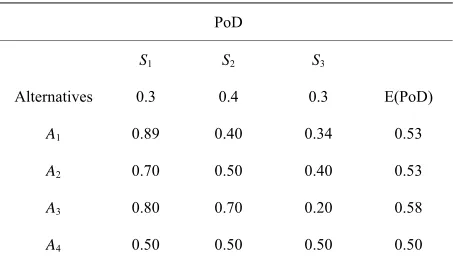
The Rational Individual who equates PoD with utility is considered to be “risk neutral”. S(he) would use Equa- tion (1) with the values in Table 2 columns 1-4 to com-
pute each sensor EU. Based on the values in Table 2
column 5, s(he) would select A3. The Rational Individual who is either risk-averse or risk-seeking would argue that utility rather than PoD is the appropriate measure of sensor usefulness. In accordance with EUT, s(he) would base his/her preferences on the MEU.
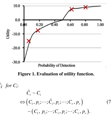
Utility is associated with the performance of an alter- native or the consequences of an act. The evaluation of a person’s utility is a highly challenging task and for great- er realism it should be experimentally solicited without invoking analytical mathematical functions [23]. The pro- cess is illustrated for a Table 2 sensor.
1) PoD = 0.5 is identified as the reference level with
u(0.5) = 0. Other values are assessed relative to it.
2) Outcomes associated with PoD > 0.5 are considered gains. The corresponding utilities have a diminishing cha- racteristic of gain satiation. For ease of perception, a scale is established with u(1.0) = 10.
3) Outcomes associated with PoD < 0.5 are considered losses. In accordance with loss aversion, the shape of the utility function is steeper than for PoD > 0.5. A lower PoD threshold may be specified to screen out unaccept- able alternatives. It is assumed that u(0) = –30.
4) The utilities of a few intermediate PoD values are determined by probing the DM about his/her indifference or willingness to bet a PoDi sensor for a 50-50 gamble
between a sensor with PoDh > PoDi and a sensor with
PoDl< PoDi. For example, consider a DM indifferent
between a PoD = 0.06 sensor and a 50-50 gamble of a PoD = 0.5 sensor or nothing, i.e. sensor with PoD = 0.
This equates to
0.06
0.5 0.5
0.5 0
0.5 30.0
15.0.u u u
Other intermediate points are determined the same way.
5) The resulting data are depicted in Figure 1. They
[image:3.595.310.537.604.735.2]can be fitted with the following utility function:
Table 2. Sensor cookie-cutter model data.
PoD
S1 S2 S3
Alternatives 0.3 0.4 0.3 E(PoD)
A1 0.89 0.40 0.34 0.53
A2 0.70 0.50 0.40 0.53
A3 0.80 0.70 0.20 0.58
A4 0.50 0.50 0.50 0.50
5The analysis can be extended to incorporate sensor physical properties
, ,
A
1
2
1 2
,
log log
0.5, 0.2, 11.49, 17
u x x x
u x x
,.57, 0.01.
x
(4)
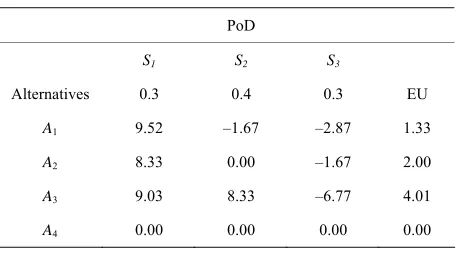
The utility values for Table 2 data are given in Table 3. Sensors A1 and A2 have unequal EUs. This reflects the fact that the utility function given by Equation (4) cap- tures some aspects of risk aversion. The Rational Indi- vidual would select A3. The rational individual, however, might disagree with this choice because of the poor per- formance of A3 in state S3. S(he) would argue that this choice is not robust because it is vulnerable to attacks by adversaries who may have acquired this information [14].
3. Limitations of the EUT Axioms
3.1. Problem Formulation
As with all theoretical models, EUT has limitations. Dif- ferent but logically equivalent sets of axioms have been proposed. Most rely extensively on the concept of mone- tary lotteries. In a 1921 lecture entitled, “Geometry and Experience,” Einstein [24, p. 233] states:
“As far as the propositions of mathematics refer to re- ality, they are not certain; as far as they are certain, they do not refer to reality.”
The above comment is equally relevant with “decision theory” substituted for “mathematics”.
This section follows Luce and Raiffa’s formulation [2] because it provides greater visibility of the probabilistic aspects of the EUT axioms than recent more abstract ma- thematical formulations. Luce and Raiffa consider five basic assumptions: 1) ordering of alternatives including transitivity; 2) reduction of compound lotteries; 3) con- tinuity; 4) substitutability6; and 5) monotonicity. The con- tinuity and independence axioms are of special interest because of their key roles for the derivations of Equations (1)-(3). As a result, they are analyzed to systematically assess their validity for critical systems.
[image:4.595.59.287.586.719.2]Consider a generic scenario, a set of n alternatives
Table 3. Sensor utility decision matrix.
PoD
S1 S2 S3
Alternatives 0.3 0.4 0.3 EU
A1 9.52 –1.67 –2.87 1.33
A2 8.33 0.00 –1.67 2.00
A3 9.03 8.33 –6.77 4.01
A4 0.00 0.00 0.00 0.00
1 n
A A
C, , C
.
C C C
, and r basic consequences 1 r .
In accordance with the ordering axiom, the consequences can be arranged in order of decreasing preference and numbered accordingly: 1 2 r Every al-
ternative can then be thought of as a lottery associated with an r-tuplet of basic consequences and probabilities q7:
1
1 1
~ , ; ; , with
1 d .
0 an 1
i i
i r r
i j
r i j j
C
q
A q C q
q
1
1
, 0,1 . . ~ ( , ; , 1 .
i r
i r i
C C C p s t
C C pC p C
C
Y X
(5)
3.2. The Continuity Axiom
For each outcome Ci, the Rational Individual8 is indif-
ferent between Ci and an alternative involving just C1
and Cr:
(6)
Ci and Ci are two different entities: i can be any
outcome of an equivalence class with certainty equiva- lent Ci [25].
Context is of the essence for validity of the continuity axiom. Taken literally, the Rational Individual should be indifferent between receiving an amount of money
, ; Death, 1
and the lottery X p p for some
probability p. Following this observation, Luce and
Raiffa [2, p. 27] write:
“When put in such bold form, some, whom we would hesitate to charge with being “irrational”, will say No... Even though the universality of the assumption is suspect, two thoughts are consoling. First, in few applications are such extreme alternatives as death present.”
Critical systems and decisions often impact life and death issues. The DM who is a rational individual cannot invoke the above loophole. S(he) needs to mindfully as- sess low probability events with potentially dire conse- quences such as serious injuries, death, and heavy finan- cial losses. The emotionally charged aspects of such de- cisions render the use of the continuity axiom impractical and unrealistic.
3.3. The Independence Axiom9
For every alternative in the set A, the Rational Individual is indifferent to the substitution of an equivalent outcome
7The variables
p and qdenote probabilities in different contexts. The variable p denotes scenario probabilities. The variable qdenotes the probabilities of the basic outcomes associated with alternatives. Equa-tion (5) refers to a generic scenario and a scenario index has been omit-ted with no loss of generality.
8The original vNM EUT axioms did not explicitly refer to the
“Ra-tional Individual”.
9The independence axiom is not one of the original vNM axioms.
Mal-invaud [25] showed that it had been implicitly assumed.
Figure 1. Evaluation of utility function.
C
; ; ,; ; , .
r r i i r r
C p
p C p
0; ;C p,
, ; , 1p Q p .
; , 1 .
p Q p
i
1 1
1 1
~
, ; ; , ~ , ; ;
,
i i
i i
C C
C p C p
C p C
for Ci:
(7a)
The independence condition given by Equation (7a) is more apparent if expressed in terms of the combination
i r r in common with arbi-
trary alternatives G or H. The independence axiom then
reduces to its common form,
1, ; ; ,1Q C p C
~ , ; , 1 ~
G H G p Q p H (7b)
It follows from the EUT continuity and transitivity axioms that
, ; , 1 ,
GH G p Q p H (7c)
The probabilistic outcomes on the right-sides of Equa- tions (7b) and (7c) are the mutually exclusive basic out- comes associated with Q, G and H. It would be wrong to
think of them as mixtures of outcomes.
The independence axiom requires that when compar- ing probabilistic alternatives, the Rational Individual views the “common part” as irrelevant and preserves the original preference in accordance with Equations (7a)- (7c). This is a valid assumption if and only if there are no interaction effects including psychological influences be- tween G and Q or H and Q. The use of decision trees is
often presented as a graphical justification for the inde- pendence axiom. This argument is flawed because the folding back procedure substitutes the certainty equiva- lent for branches at nodes and thereby implicitly assumes that outcomes are independent. De Neuville [26, p. 366] writes:
“The axiom implies that the substitutions can occur re- gardless of the other opportunities in front of a person and, thus, regardless of how these substitutions alter the probabilistic distribution of the consequences.”
In conclusion, the independence axiom is in conflict with probability calculus and the rational individual who
makes decisions based on the complete risk curve rather than simply the EU [27].
3.4. The Chew Weighted Utility Theory
The Chew weighted utility theory [28] replaces the inde- pendence axiom with the weak substitution axiom:
, , , ~ 0,1 , 0,1
. . , ; , 1 ~ , ; , 1 .
i j k i j
i k j k
A A A A A A
s t A A A A
(8)
For the weak substitution axiom reduces to the independence axiom, Equation (7b). The Chew wei- ghted utility theory includes EUT as a special case. For
it admits the presence of complementarities of Ai
and Aj with Ak. It, therefore, provides a resolution of the
Allais paradox [29] as well as the two-sensor paradox of Section 4.
The Chew weighted utility function for a probabilistic mixture of two alternatives H and G has the following
linear functional form:
1
1
. 1wut pW H U H p W G U G
U pH p G
pW H p W G
(9)
U is a vNM utility function; W is an addi-
tional weight function that enables it to accommodate the preference patterns of several key EUT paradoxes in- cluding the Allais paradox [29]. Equation (9) reduces to Equation (1) for
W Constant. Otherwise, it signi-
ficantly increases the complexity of EUT, which limits its applicability as a normative model for AoAs.
3.5. Choice Axioms for Catastrophic Risks
As discussed in Section 2, the EUT linear functional form causes the ranking of alternatives to be relatively insensitive to low probability scenarios. This is in con- flict with the way rational individuals often choose op- tions for a wide range of problems with low probability but catastrophic consequences. These include, but are not limited to, global environmental risks, national security, and critical infrastructures. Chichilnisky [13] proposed a set of 3 axioms to account for such choices. It results in a utility function W
that includes a term that assignspositive weights to low probability events:
vNM 1
,
W x U x x
x y W x W y
0 1
(10)
4. Two-Sensor Paradox
The Section 2.2 sensors are considered for a border sur- veillance system of length 4R0. The problem is which two sensors to select to maximize the detection probabil- ity of potential intruders. It is assumed that the latter possess no intelligence of sensor performance; they try to infiltrate the border at random locations and times.
4.1. EUT Analysis For the Rational Individual,
1
i
1
j.i j i i
A A pA p A pA p A (11)
S(he) would then conclude that the homogeneous com- bination AiAi is preferable to the hybrid combination
i j
A A . By extending this reasoning to all sensor com-
binations, the Rational Individual concludes that the best combination consists only of the highest utility sensor, i.e. A3. The rational individual would disagree with this solu-
tion because it lacks diversity and it is highly vulnerable to infiltration given the low PoD in scenario S3 (see Ta- ble 2). There are several other examples of EUT par-
adoxes with anomalous risk behaviors [30-31].
4.2. Two-Dimensional Preference Analysis
Given 4 alternatives, there are 10 possible two-sensor combinations to consider. Each combination
A Ai, j
may be represented by a two-dimensional vector with the PoD utility as elements. A two-dimensional utility func- tion is needed to represent preferences over the combina- tions such that
, j
k, l
., ,
i j k l i
A A A A U x x U x x (12)
By analogy to the determination of the sensor utility function in Section 2.2, it is assumed that U x
,y isgiven by treating Equation (4) as a function of the joint variable xy:
1
2
1 2
, ,
, log l
0.5, 0.2, 11.49, 17.57
D D
U x y xy x
U x y xy
.
og ,
, 0.01
x
(13)
The multiplicative form xy has advantages over the
linear form xy . It more realistically accounts for
two-sensor vulnerabilities. Furthermore, the D
,y
U x
indifference or isoutility curves represent simple convex preferences10.
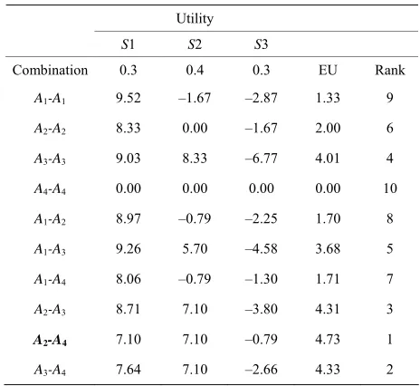
[image:6.595.306.538.99.312.2]The utilities for the 10 two-sensor combination are computed using Equation (13) and averaged over the 3 scenarios. The results are presented in Table 4.
Table 4. Two-dimensional preference analysis.
Utility
S1 S2 S3
Combination 0.3 0.4 0.3 EU Rank
A1-A1 9.52 –1.67 –2.87 1.33 9
A2-A2 8.33 0.00 –1.67 2.00 6
A3-A3 9.03 8.33 –6.77 4.01 4
A4-A4 0.00 0.00 0.00 0.00 10
A1-A2 8.97 –0.79 –2.25 1.70 8
A1-A3 9.26 5.70 –4.58 3.68 5
A1-A4 8.06 –0.79 –1.30 1.71 7
A2-A3 8.71 7.10 –3.80 4.31 3 A2-A4 7.10 7.10 –0.79 4.73 1
A3-A4 7.64 7.10 –2.66 4.33 2
1) A2A4A3A3. The MEU solution, A2A4, does not consist of the two MEU alternatives. It draws on the synergistic interaction between the two alternatives.
2) D ·
U
and
i k j k
exhibits diversification [32]. For some combinations ofA A A A ,
, 1
.D D
i j k
U pA p A U A (14)
3) The robust combination A4-A4ranks last. This result combined with the above two demonstrates that convex preferences exhibit diversification but that diversification is not equivalent to robustness.
A resolution of the two-sensor paradox is that EUT needs to be modified to be compatible with preference for robust and hybrid solutions. Options include 1) re- placing the independence axiom with a modification such as the weak substitution axiom, or 2) introducing correc- tions to EUT such as DT (see Section 6).
5. Robust Solutions
5.1. Various Notions
In semi-layman parlance, robust solutions perform rea- sonably well and have acceptable outcomes over a wide range of plausible scenarios without assuming that “eve- rything goes right”. The importance of robustness as a criterion for good decisions is reflected by the fact that DMs often purposefully forgo the MEU option for ones that perform well over a wide range of scenarios and are relatively insensitive to uncertainties. The professional literature contains different notions of robustness with variations that depend on the application domain.
The following three notions of robustness are of inter- est for critical systems consideration.
10The key property of convex preferences is that any point on the
straight line joining two points on the same indifference curve has a higher utility than either point. A person with convex preferences
with relatively small regret compared to the alternatives across a wide range of plausible futures.” They evaluate the regret of long-term policies using an approach based on Savage’s minimax regret rule11.
2) Krokhmal et al. [34] advocate generating robust de-
cision by optimizing an upper percentile of the risk prob- ability distribution12. They note that “in this regard, risk management in military applications is similar to other fields such as finance, nuclear safety, etc., where deci- sions targeted at achieving the maximal expected perfor- mance may lead to an excessive risk exposure.”
3) Ullman [35] advocates developing designs with low sensitivity to noise or uncertainty in accordance with the Taguchi method. He considers performance, risk and cost among the factors that need to be addressed [35, p. 36]: “The result of a robust decision is an option chosen with known and acceptable satisfaction and risk... A major goal in making a robust decision is to eliminate all the uncertainty possible within the scope of available re- sources.”
This section examines Savage’s minimax regret rule as a regret-based robustness criterion. Risk-based robust- ness is addressed in Section 6.
5.2. The Minimax Regret Rule
Savage’s minimax regret rule is a recommendation that under uncertainty a person should choose the alternative that minimizes the maximum difference from the highest achievable utility in each scenario. The anticipated regret for choice Ai in scenario Sj depends on the other alterna-
tives:
,
Max
,
,
,l
i j l j i j
A
R A S U A S U A S
,
U A S
(15a)
where l j is a vNM utility. Equation (15a) re-
presents the largest possible loss for Ai in state Sj relative
to the best alternative. The minimax regret choice is the alternative A with the smallest regret over all of the
scenarios:
1
x , Min Max , , , , .
i
j j
j i j n
A
S R A S S R A S A A A
Ma
(15b) The minimax regret rule leads to the comparison of the
Table 3 sensors in Table 5. Sensor A3 is the recom-
mended alternative; but, it performs poorly in S3. The
rational individual who seeks a robust solution is likely to reject it. The well balanced A4 ranks3rd. These results
raise serious doubts about the usefulness of the minimax regret rule as a robustness criterion13.
The maximin criterion, also known as Wald’s mini- max for losses, recommends selecting the alternative with the maximum minimum utility, A4 (see Table 3).
The maximin criterion and minimax regret criterion have different characteristics. The maximin criterion captures aversion to the worst possible outcome for each alterna- tive. The minimax regret criterion is concerned with missing beneficial opportunities. Numerous analysts be- lieve that the minimax regret criterion is preferable to the maximin criterion; this is in conflict with the above re- sults.
6. Disappointment Theory for AoA
The term “disappointment” has psychological connote- tions that are not relevant in the context of the paper. Nevertheless, it is used in the paper because it is en- trenched in the decision theory literature.
6.1. General Overview
Bell [10] and Loomes and Sugden [11] proposed DT to account for the fact that rational individuals may antici- pate disappointment when they counterfactually compare the outcome of an action in one scenario relative to the better outcomes in the other scenarios. The rational indi- vidual may account ex-ante for these negative feelings in
decision making. Similarly, feelings of elation are asso- ciated with the better outcomes. DT, unlike RT, does not perform comparisons across alternatives. This avoids potentially misleading results of pairwise comparisons [36]. The disappointment level and utility of an alterna- tive are therefore independent of the other alternatives.
[image:7.595.309.537.576.715.2]Several DT models have been proposed as corrections to EUT. Bell [10] and Loomes and Sugden [11] assumed that for a given alternative the strength of the disappoint- ment associated with a probabilistic outcome is measured relative to the alternative’s EU. Delquié and Cillo [37] noted that rational individuals are more likely to compare
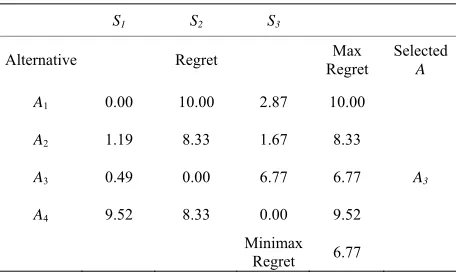
Table 5. The minimax regret decision matrix corresponding to Table 3.
S1 S2 S3
Alternative Regret Regret Max Selected A
A1 0.00 10.00 2.87 10.00
A2 1.19 8.33 1.67 8.33
A3 0.49 0.00 6.77 6.77 A3
A4 9.52 8.33 0.00 9.52
Minimax
Regret 6.77
11Savage [4, p. 163] objected to use of the term “regret” and used
“loss” instead. Referring to “regret”, he writes “that term seems to me to be charged with emotion and liable to lead to such misinterpretation as that the loss necessarily becomes known to the person”.
12The percentile is one of several mathematical criteria used for
“con-ditional value-at-risk”.
13For completeness, it is noted that there are other serious problems
the outcome obtained against the outcomes that they failed to get had other scenarios realized. They hypothe- sized that the level of disappointment associated with outcome Oi depends explicitly on the probabilities and
utilities of the outcomes that are preferred, i.e. the out-
comes k
14. The disappointment associ- ated with alternative Aj given the realization of scenario
Si, is modeled as follows:
, 1, , i1
vNM , ,
j i
A S
D
f
O k
vNM
1
, i ,
j i k D j k k
DT A S p f U A S U
(16) where is a positive function of UvNM
with; is the probability of scenario Sk.
0 0 pk
f
, ,
,k i k i j
p u u
, 1, ,
D
f
6.2. Disappointment Correction to EUT
For the purpose of this paper, D in Equation (16) is
assumed to be a linear function. The overall disappoint- ment is then obtained by averaging Equation (16) over all the m scenarios. This simplified version of the Delquié
and Cillo Linear Disappointment Model (LDM) [37] modifies the vNM EU, Equation (2), as follows:
LDM
,
1 1
EU i m j i j d j
j k
A p u
(17)where d is a positive constant that captures the rational individual’s sensitivity to disappointment.
Equation (17) has several notable properties:
1) The functional form is similar to the vNM EU but with rank-dependent weighted probabilities.
2) The second term represents downside risk15 relative to the best possible outcome. It provides a credible meas- ure of risk-based robustness.
3) The parameter d can be varied to reflect varying degrees of risk tolerance and thereby identify alternatives with unacceptable consequences.
6.3. Two-Sensor Selection Example
The two-sensor paradox of Section 4 is analyzed using the LDM. Given that disappointment is explicitly ac- counted for, the analysis uses the Table 2 physical data.
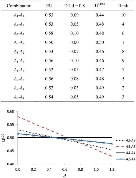
The results for d = 0.8 are presented in Table 6. Figure 2
compares several two-sensor combinations versus d. The results are consistent with a rational preference for diversification and the notion of risk-based robustness. The two-sensor combinations change rank as d varies. For d > 0.7, A4-A4 rank 1st and A2-A4 ranks 2nd. A3-A3
changes rank from 1stfor d = 0 to last for d > 0.6. To reach a final decision, a risk-averse DM would peruse
Figure 2 and chooses between.A2-A4 or A4-A4 depending
on preferences for risk tolerance and diversification. The LDM16 analysis is simpler and more intuitive than the utility theory two-dimensional preference analysis of Section 4.2. It can readily be extended to complex com- binations of multiple constituents. However, all available DT models lack a mathematical basis for developing complex hybrid solutions or portfolios. Such an approach is presented in the next section.
7. Portfolio Optimization for Robustness
7.1. General Formulation
As discussed in Sections 4-6, a risk-adverse DM is likely to prefer a hybrid solution that performs relatively well over all scenarios of interest rather than a homogeneous solution consisting solely of the MEU alternative. Con- sider a situation of n alternatives A ii n and m
mutually exclusive probabilistic scenarios
Sj,pj, j1, , m
. A hybrid solution may be thought [image:8.595.308.539.372.674.2]of as a portfolio characterized by a multidimensional probability distribution function [39],
Table 6. Results using the linear disappointment model.
Combination EU DT d = 0.8 ULDM Rank
A1-A1 0.53 0.09 0.44 10
A2-A2 0.53 0.05 0.48 4
A3-A3 0.58 0.10 0.48 6
A4-A4 0.50 0.00 0.50 1
A1-A2 0.53 0.07 0.46 8
A1-A3 0.56 0.10 0.46 9
A1-A4 0.52 0.05 0.47 7
A2-A3 0.56 0.08 0.48 5
A2-A4 0.52 0.03 0.49 2
A3-A4 0.54 0.05 0.49 3
0.40 0.45 0.50 0.55 0.60
0.0 0.2 0.4 0.6 0.8 1.0 1.2
U
LD
C
d
[image:8.595.308.539.372.676.2]A2‐A2 A3‐A3 A4‐A4 A2‐A4
Figure 2. Comparison of selected two-sensor combinations versus disappointment parameter d using the linear disap- pointment model.
14The outcome
Oi is associated with scenario Si. It is convenient to
number the outcomes, and thereby the scenarios, in order of decreasing preference. This ordering is used throughout the section.
15Downside risk is a proven measure for characterizing portfolio risk
[38].
16Simplicity and descriptive realism are two key objectives of DT [10,
1 1
n m
HS i pd
i j
P x x F f
A Si, j
,pj ,
, , ,
(19a)
where x x1 2 xn
x is the decision vector of allo-
cation variables with xi being the Ai allocation fraction.
The multidimensional function F
,is a generalized discrete probability distribution with values being prob- ability distributions functions (pdf) rather than point es-timates. pd i j
is a pdf that models the Ai out-come17 for scenario
Sj.
f A
1
n i i
x S
The determination of the decision vector x may be
specified in terms of the following stochastic optimiza- tion problem:
Maximize the th percentile of PHS(x), Equation (19a),
subject to the normalization, scenario performance, and affordability constraints, Equations (19b)-(19d):
,
d A Sj j S
(19b)
1
percentile of , j n i t
p i h
i
R S x f j
x
0 0
1
.
n i i i
x C B
, , ,
(19c)
T
C x N (19d)
The values and are percentiles18 that a DM speci- fies in accordance with his/her risk tolerance; j is
his/her lowest acceptable value for the th percentile for performance in scenario Sj; Ci is the Ai cost; N0 is the number of required systems; and B0 is the available budget. Equation (19d) can accommodate pdfs for Ci
with an agreed-to percentile for the cost constraint [27]. The above formulation provides a flexible and trans- parent way for the analyst and DM to define the choice problem and generate mixed solutions with desirable pro- perties such as diversification and robustness19.
7.2. Hybrid Solution Example
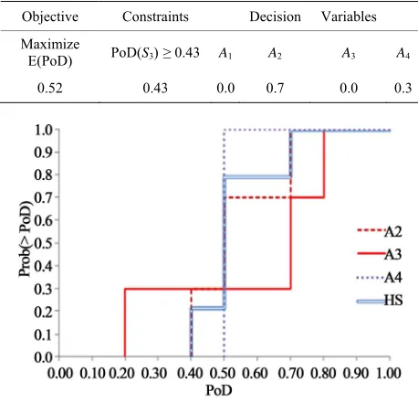
The above approach is applied to the design of a robust border surveillance system of N0 sensors using the four
Table 2 sensors. The problem is to determine the com-
[image:9.595.307.539.100.322.2]bination of sensors 1 2 3 4
Table 7. Sensor hybrid solution optimized for robustness.
Objective Constraints Decision Variables Maximize
E(PoD) PoD(S3)≥ 0.43 A1 A2 A3 A4
0.52 0.43 0.0 0.7 0.0 0.3
Figure 3. Cumulative distributions for the hybrid sensor solution (HS) optimized for robustness, its constituent sen- sors A2 and A4, and the MEU alternative A3.
The hybrid solution is robust: 1) the associated cumula- tive distribution is narrower than those of the homoge- neous alternatives, 2) the minimum PoD = 0.4, and 3) there is a 80% probability that the PoD 0.5 for the identified scenarios. Given the Table 2 alternatives, this
is the solution that a DM who desires some level of ro- bustness at an acceptable performance cost is likely to intuitively prefer. Diversity provides additional benefits such as defense against common-cause failures [42] and increased deterrence against attackers [14].
The solution to this example is obvious. Nevertheless, it illustrates the significant advantages and benefits of portfolio allocation with stochastic optimization for de- veloping robust critical systems. Solving complex real- world problems will require tools with integrated Monte Carlo simulation and stochastic optimization capabilities. They are available in commercial and proprietary ver- sions. For information purposes, Crystal Ball®with Opt- Quest®was applied to the illustrative example. OptQuest® is a general purpose optimizer developed to effectively solve complex stochastic, nonlinear, and combinatorial optimization problems [43].
x x x x
S S S, ,
PoD S 0.43, Equation (19a), that maximizes the expected PoD over the three scenar- ios 1 2 3 subject to the normalization constraint,
Equation (19b), and 3 for the perform- ance constraint, Equation (19c). The budget is assumed not to be a constraint. The hybrid solution data are sum- marized in Table 7 and its cumulative distribution [41]
and several of interest are depicted in Figure 3.
8. Conclusions
The paper begins by analyzing the suitability of EUT for AoAs of critical systems in a multistate world. The con- cept of robust solutions is discussed within the context of multiple scenarios. Several well-known models are com- pared for a simplified example of choosing sensors for a hypothetical border surveillance system. Portfolio allocation
17Given complex systems, realistic scenario outcomes have significant
uncertainties that need to be accounted for distinct from the scenario probabilities.
18Expected values are included.
19“Robustness,” as used in this paper (see Section 5), is an attribute of
[image:9.595.308.537.101.321.2]with stochastic optimization is proposed and demon- strated to be a valid and realistic method for defining robust critical systems.
Some of the key conclusions are:
1) The EUT is inadequate for critical systems AoA because MEU alternatives may possess vulnerabilities that could be exploited and/or are susceptible to com- mon-cause failures. The continuity axiom is unrealistic given the emotionally charged aspects of critical deci- sions. The independence axiom is in conflict with the rational individual who is not an expected utility maxi- mizer and prefers to make decisions using risk curves.
2) The two-sensor paradox raises serious doubts about the validity of the minimax regret rule as a robustness criterion for decision making under risk and the belief that it is superior to the maximin rule. Both have serious problems and are potential misleading for choosing criti- cal systems.
3) If the utility is linear in the probabilities, the EU of a hybrid solution cannot be greater than the EU of every constituent alternative. A GEUT and nonlinear utility functions are required to exhibit robustness and diversi- fication.
4) The LDM simply modifies the vNM EU by adding a term proportional to downside risk. The results of the two-sensor selection example confirm that it is a promis- ing model for choosing robust homogeneous solutions. However, the LDM and other available DT models do not provide a mathematical basis for developing hybrid solutions.
5) Portfolio allocation with stochastic optimization provides a flexible and transparent approach for defining the choice problem and determining hybrid solutions for critical systems with desirable properties such as diversi- fication and robustness. The best combination does not necessarily consist of the alternatives with the highest EUs; it draws on the strengths and complementarities that any of the alternatives can provide.
6) The composition of the hybrid solution is deter- mined by optimizing a specified percentile of the system performance subject to robustness and cost constraints. Performance and cost uncertainties can be modeled using realistic pdf’s.
Ultimately, the selection of robust solutions depends on the identified alternatives. Critical systems require analysis that is mindful of the following considerations: 1) the limitations of EUT and GEUT models; 2) risk-miti- gation properties such as FARness; and 3) the impor- tance of hybrid solutions as options. Given the availabil- ity of commercial and proprietary tools with integrated Monte Carlo simulation and stochastic optimization ca- pabilities, the future direction is the implementation of the proposed portfolio allocation with stochastic optimi- zation as a practical design and analysis tool for complex
systems and SoS on actual projects.
9. Acknowledgments
This work was stimulated by a Naval Postgraduate School capstone project prepared by the 2008 Cohort from the Naval Surface Warfare Center Dahlgren Divi- sion (NSWCDD) and the Naval Undersea Warfare Cen- ter Division Newport [44]. The author thanks Neil Baron, Distinguished Scientist NSWCDD, for insightful com- ments on hybrid solutions.
EFERENCES
[1] US Office of Homeland Security, “The National Strategy for Homeland Security,” 2002.
http://www.ncs.gov/library/policy_docs/nat_strat_hls.pdf [2] R. D. Luce and H. Raiffa, “Games and Decisions: Intro-
duction and Critical Survey,” Dover Publications, New York, 1957.
[3] J. von Neumann and O. Morgenstern, “Theory of Games and Economic Behavior,”2nd Edition,Princeton Univer- sity Press, Princeton, 1947.
[4] L. J. Savage, “The Foundations of Statistics,” 2nd Re- vised Edition, Dover Publications, New York, 1972. [5] P. C. Fishburn, “Normative Theories of Decision Making
under Risk and Uncertainty,” In: D. Bell, H. Raiffa and A. Tversky, Eds., Decision Making: Descriptive, Normative, and Prescriptive Interactions, Cambridge University Press, Cambridge, 1988, pp. 78-98.
doi:10.1017/CBO9780511598951.006
[6] D. Kahneman and A. Tversky, “Prospect Theory: An Ana- lysis of Decisions under Risk,” Econometrica, Vol. 47, No. 3. 1979, pp. 263-291. doi:10.2307/1914185
[7] A. Tversky and D. Kahneman, “Advances in Prospect Theory: Cumulative Representation of Uncertainty,” Jour- nal of Risk and Uncertainty, Vol. 5, No. 4, 1992, pp. 297-323.
[8] D. E. Bell, “Regret in Decision Making under Uncer- tainty,” Operations Research, Vol. 30, No. 5, 1982, pp. 961-981. doi:10.1287/opre.30.5.961
[9] G. Loomes and R. Sugden, “Regret Theory: An Alterna- tive Theory of Rational Choice under Uncertainty,” Eco- nomic Journal, Vol. 92, No. 368, 1982, pp. 805-824.
doi:10.2307/2232669
[10] D. E. Bell, “Disappointment in Decision Making under Uncertainty,” Operations Research, Vol. 33, No. 1, 1985, pp. 1-27. doi:10.1287/opre.33.1.1
[11] G. Loomes and R. Sugden, “Disappointment and Dyna- mic Consistency in Choice under Uncertainty,” Review of Economic Studies, Vol. 53, No. 2, 1986, pp. 271-282. doi:10.2307/2297651
[12] E. Dekel and B. L. Lipman, “How (Not) to Do Decision Theory,” Annual Review of Economics, Vol. 2, No. 1, 2010, pp. 257-282.
doi:10.1146/annurev.economics.102308.124328
under Uncertainty with Catastrophic Risks,” Resource and Energy Economics, Vol. 22, No. 3, 2000, pp. 221- 231. doi:10.2139/ssrn.1522307
[14] G. G. Brown and L. A. Cox Jr., “Making Terrorism Risk Analysis Less Harmful and More Useful: Another Try,” Risk Analysis,Vol. 31, No. 2, 2011, pp. 193-195. doi:10.1111/j.1539-6924.2010.01563.x
[15] P. K. Davis, R. D. Shaver and J. Beck, “Portfolio-Analy- sis Methods for Assessing Capability Options,” RAND, Santa Monica, 2008.
[16] S. Savage, “The Flaw of Averages: Why We Underesti- mate Risk in the Face of Uncertainty,” John Wiley & Sons, Hoboken, 2009.
[17] Y. Y. Haimes, “Risk Modeling, Assessment, and Man- agement,” 3rd Edition, John Wiley & Sons, Hoboken, 2009.
[18] H. M. Markowitz, “Portfolio Selection: Efficient Diversi- fication of Investments,” 2nd Edition, Blackwell, Cam- bridge, 1997.
[19] Office of the Deputy under Secretary of Defense for Ac- quisition and Technology, Systems and Software Engi- neering, “Systems Engineering Guide for Systems of Sys- tems,” Version 1.0, ODUSD(A&T)SSE, Washington, 2008. [20] D. H. Wagner, W. C. Mylander and T. J. Sanders, “Naval
Operations Analysis,” 3rd Edition, Naval Institute Press, Annapolis, 1999.
[21] A. Washburn and M. Kress, “Combat Modeling,” Sprin- ger, New York, 2009. doi:10.1007/978-1-4419-0790-5
[22] 2011 Naval Surface Warfare Center Crane Cohort, “Sys- tem Engineering Approach to Improving Arizona Border Patrol C4ISR Mission Operations,” MSSE Capstone Pro- ject, Naval Postgraduate School, Monterey, 2011. [23] R. Hastie and R. M. Dawes, “Rational Choice in an Un-
certain World: The Psychology of Judgment and Decision Making,” Sage Publications, Thousand Oaks, 2001. [24] A. Einstein, “Ideas and Opinions,” Bonanza Books, New
York, 1954.
[25] E. Malinvaud, “Note on von Neumann-Morgenstern’s Strong Independence Axiom,” Econometrica, Vol. 20, No. 4, 1952, p. 679. doi:10.2307/1907650
[26] R. de Neuville, “Applied Systems Analysis: Engineering Planning and Technology Management,” McGraw-Hill, New York, 1999.
[27] E. Kujawski, M. Alvaro and W. Edwards, “Incorporating Psychological Influences in Probabilistic Cost Analysis,” Systems Engineering, Vol. 7, No. 3, 2004, pp. 195-216. doi:10.1002/sys.20004
[28] S. H. Chew, “Axiomatic Utility Theories with the Betwe- enness Property,” Annals of Operations Research, Vol. 19, No. 1, 1989, pp. 273-298. doi:10.1007/BF02283525
[29] M. Allais, “Le Comportement de l’Homme Rationnel devant le Risque: Critique des Postulats et Axiomes de l’Ecole Américaine,” Econometrica, Vol. 21, No. 4, 1953, pp. 503-546. doi:10.2307/1907921
[30] P. Samuelson, “Risk and Uncertainty: A Fallacy of Large Numbers,” Scientia, Vol. 98, No. 4, 1963, pp. 108-113. [31] M. Rabin and R. H. Thaler, “Anomalies: Risk Aversion,”
The Journal of Economic Perspectives, Vol. 15, No. 1, 2001, pp. 219-232. doi:10.1257/jep.15.1.219
[32] E. Dekel, “Asset Demands without the Independence Axi- om,” Econometrica, Vol. 57, No. 1, 1989, pp. 163-169. doi:10.2307/1912577
[33] R. J. Lempert, D. G. Groves, S. W. Popper and S. C. Bankes, “A General, Analytic Method for Generating Ro- bust Strategies and Narrative Scenarios,” Management Science, Vol. 52, No. 4, 2006, pp. 51-528.
doi:10.1287/mnsc.1050.0472
[34] P. Krokhmal, R. Murphey, P. Pardalos, S. Uryasev and G. Zrazhevsky, “Robust Decision Making: Addressing Un- certainties in Distributions,” In:S. Butenko, et al., Eds., Cooperative Control: Models, Applications and Algori- thms, Kluwer Academic Publishers, Dordrecht, 2003, pp. 165-185.
[35] D. G. Ullman, “Making Robust Decisions: Decision Man- agement for Technical, Business, & Service,” Trafford Publishing, Victoria, 2006.
[36] G. Friedman, “The Intransitivity of Pairwise Comparisons Even with a Single Rational Decision Maker or: Homo- morphisms from Allegedly Paradoxical Dice to Deci- sion-Making in the Military, Business and Sports World,” Presentation to the NSF Decision-Based Design Work- shop, Long Beach,1999.
http://dbd.eng.buffalo.edu/papers/friedman.html
[37] P. Delquié and A. Cillo, “Disappointment without Prior Expectation: A Unifying Perspective on Decision under Risk,” Journal of Risk and Uncertainty, Vol. 33, No. 3, pp. 197-215. doi:10.1007/s11166-006-0499-4
[38] D. Nawrocki, “A Brief History of Downside Risk Meas- ures,” Journal of Investing, Vol. 8, No. 3, 1999, pp. 9-25. doi:10.3905/joi.1999.319365
[39] E. Kujawski and G. A. Miller, “Quantitative Risk-Based Analysis for Military Counterterrorism Systems,” Systems Engineering, Vol. 10, No. 4, 2007, pp. 273-289.
doi:10.1002/sys.20075
[40] D Bertsimas, D. B. Brown and C. Caramanis, “The The- ory and Applications of Robust Optimization,” SIAM Re- view, Vol. 53, No. 3, 2011, pp. 464-501.
doi:10.1137/080734510
[41] M. Levy, “Almost Stochastic Dominance and Efficient Investment Sets,” American Journal of Operations Re- search, Vol. 2, No. 3, 2012, pp. 313-321.
doi:10.4236/ajor.2012.23038
[42] E. Kujawski, I. M. Jacobs and A. M. Smith, “An Evalua- tion of the Use of Signal Validation Techniques as a De- fense against Common-Cause Failures,” Electric Power Research Institute, Palo Alto, 1987.
[43] F. Glover, M. Laguna and R. Martí, “Scatter Search,” In: A. Ghosh and S. Tsutsui, Eds., Advances in Evolutionary Computation: Theory and Applications, Springer-Verlag, New York, 2003, pp. 519-537.