Munich Personal RePEc Archive
What blows in with the wind?
De Silva, Dakshina G. and McComb, Robert P. and Schiller,
Anita R.
Texas Tech University
3 November 2014
Online at
https://mpra.ub.uni-muenchen.de/59663/
What blows in with the wind?
Dakshina G. De Silva
yRobert P. McComb
zAnita R. Schiller
xNovember 3, 2014
Abstract
The shift toward renewable forms of energy for electricity generation in the electricity gener-ation industry has clear implicgener-ations for the spatial distribution of generating plant. Traditional forms of generation are typically located close to the load or population centers, while wind and solar-powered generation must be located where the energy source is found. In the case of wind, this has meant signi…cant new investment in wind plant in primarily rural areas that have been in secular economic decline. This paper investigates the localized economic impacts of the rapid increase in wind power capacity at the county level in Texas. Unlike Input-Output impact analysis that relies primarily on levels of inputs to estimate gross impacts, we use traditional econometric methods to estimate net localized impacts in terms of employment, personal income, property tax base, and key public school expenditure levels. While we …nd evidence that both direct and indi-rect employment impacts are modest, signi…cant increases in per capita income accompany wind power development. County and school property tax rolls also realize important bene…ts from the local siting of utility scale wind power although peculiarities in Texas school funding shift localized property tax bene…ts to the state.
JEL Classi…cation: H23, H72, Q42, Q48, R11.
Keywords: wind energy, industry studies, per capita income, public sector revenues and expen-ditures.
1
Introduction
Global growth of wind powered electricity generation in the last decade has been substantial. In the
United States alone, according to the National Renewable Energy Laboratory, installed wind power
capacity has increased from 2,539 MW in year 2000 to 61,108 MW by year-end 2013. Although
most wind generation is concentrated across the Great Plains, Midwest, and Far West regions of
We would like to thank Geo¤rey Hewings, Xiaoyi Mu, participants at the Western Economic Association Interna-tional, 2013 Annual Conference and two anonymous referees for valuable comments and suggestions. We also would like thank the Texas Workforce Commission for providing the data and the Texas Tech University National Wind Insitute
for their ongoing research support.
yDepartment of Economics, Lancaster University Management School, Lancaster University, Lancaster, LA1 4YX,
UK (e-mail: [email protected]).
zCorresponding author: Department of Economics, Texas Tech University, MS: 41014, Lubbock, TX 79409-1014,
(e-mail: [email protected]).
xCentre for Energy, Petroleum and Mineral Law and Policy, Graduate School of Natural Resources Law, Policy and
the U.S., nearly 39 states now have utility-scale wind powered electricity generation. As turbine
technology continues to improve, with concomitant reductions in generating costs, the geographic
range of economically feasible generation will expand. Mounting economic and political pressure to
increase the share of clean, renewable energies in the nation’s electrical power generation portfolio will
likely pave the way for build-out of high voltage power transmission from high quality wind resources
to populous regions.
While the main appeal of wind generation is its environmental bene…t, it also o¤ers a di¤erent
industrial trajectory that is seen as having the potential to bestow bene…ts on new constituencies.
Indeed, the spatial distribution of utility-scale electricity generation among the di¤erent types of
elec-trical generation is quite di¤erent and thus implies a corresponding change in the spatial distribution
of employment (at the point of generation) and, possibly, income. Thermal generation, the
domi-nant form of electricity generation, is typically located close to load centers, i.e., more populous areas;
whereas wind generation must necessarily be located where the wind resource is found. A casual glance
at a wind resource map suggests that these wind resource-rich regions tend to be more rural, exhibiting
relatively low population densities. This has meant, among other things, a sharp uptick in …xed plant
in some windy rural areas that have been in secular decline and increased investment in transmission
capacity to exploit the wind resources and deliver the energy to urban consumers.
It is therefore not too surprising that rural development interests have been allied with
environ-mental groups at the forefront of political advocacy for policies to promote growth of wind generation.
There are, of course, both short and long-term bene…ts and costs associated with this development
that need to be considered before net localized bene…ts can be identi…ed. However, the extent of net
localized economic impacts has not been widely studied.
In this paper, we investigate the localized economic e¤ects of wind power development. We use
the State of Texas as the region for analysis. We are able to exploit the controlled comparison
enabled by the fact that Texas has large regions with high quality wind resources and (otherwise
similar) large regions with uneconomic wind regimes to identify wind power-related changes in the
variables of interest. Rather than relying on an input-output modeling methodology to extrapolate
gross outcomes, we consider the net localized spillover e¤ects on other industrial employment, per capita
using standard regression analysis. Unlike previous research in this area, we conduct an analysis that
seeks to observe the nature of employment growth in terms of its industrial composition and the likely
inter-industry spillovers. Although we are unable to observe directly whether or not the increases in
tax capacity result in higher levels of local public goods provision, we consider the question of changes
in levels of per-student public education expenditures as an indirect measure of changes in levels in
local public goods.1 This paper is the …rst to examine the net e¤ects of wind energy development on
school tax rates, revenues and expenditures.
Restricting the analysis to Texas still captures a signi…cant share of the wind power industry. Over
20 percent of the total installed wind generation capacity in the United States at the end of 2013 was
located in Texas. With 12,355 megawatts (MW) of installed wind generation capacity at year-end
2013, Texas produces more wind generated electricity than any other state in the United States. The
rapid growth of this industry in Texas has mirrored that of the U.S. In year 2001, Texas had only 898
MW of installed wind capacity.2
By limiting the analysis to a single state, we have a consistent means by which to consider changes
in property tax bases, rates, and public school …nance. We seek to determine what, if any, persistent
local bene…ts accrue to the residents of the counties in which the wind power generation is located.
We …nd that, at best, direct and indirect employment e¤ects are modest while increases in per capita
county personal income can be important. This result implies that gains in personal income come
from sources other than wage income such as net lease income for farmers and ranchers. As expected,
we …nd that the value of county property tax bases increases with increases in installed wind capacity.
This appears to enable county governments to reduce tax rates while the bene…ts to school districts
are mitigated due, probably, to the state and local school funding formula in Texas.
It should also be noted that, since the utility-scale wind developments are non-locally owned, the
lion’s share of bene…ts will accrue outside the locality while many of the costs are borne locally.
The e¤ects on (non-migratory) avian populations, noise pollution, degradation of the landscape, and
1Beginning with Oates (1968), public education expenditures have been widely used as a proxy for the level of provision of local public goods. More recently, Weber, Burnett, and Xiarchos (2014) …nd that the larger property tax base that resulted from shale oil development in Central Texas led to increased school expenditures.
reductions in agricultural and tourism activities that accompany utility-scale wind development are
detrimental to the welfare of the local residents. The long-term consequences for land-use and the
landscape will depend on the disposition of the turbines and their foundations when their economic
life is over. We do not correct our impact analysis to take these costs into consideration.
While production technologies and supply chains are clearly quite di¤erent between the di¤erent
means of generating electricity, it is not obvious how the substitution of wind-powered generation for
generation by other energy sources will in‡uence overall employment and income in the electricity
generation sector. For example, employment in thermal generation of electricity includes activities
in fuel extraction, processing and transportation while no fuelper se is required for wind generation.
Comparing macro-level employment and income e¤ects from the shift to renewable forms of electricity
generation is complex and beyond the scope of this paper.
Of course the substitution of renewable energy sources for fossil fuels provides environmental
ben-e…ts in terms of reduced emissions of carbon dioxide, sulfur dioxide, and mercury. These are for the
most part global bene…ts. Moreover, wind power does not require water to generate electricity, a big
advantage in Texas and the Southwest. No e¤ort is made to quantify the broader environmental value
of substituting wind power for gas or coal-powered generation nor is any attempt made to establish
the e¤ect on market prices of electricity of mandated changes in the electrical generation portfolio.
The paper is organized as follows. Section 2 provides a discussion of the economic and institutional
context with a brief literature review. Section 3 describes the data and empirical models that are used
to estimate the localized economic impacts. Section 4 provides a brief discussion and conclusions.
2
The Economic and Institutional Context
The growth of wind power in Texas, as in the United States, appears to have resulted primarily
from the presence of the high quality wind resource, improvements in turbine performance, and the
assured, ex ante availability of the federal Production Tax Credit (PTC) that was enacted in 2006.3
Since installed capacity in Texas has already exceeded the requirements of the state’s 2025 Renewable
Portfolio Standard (RPS), the RPS does not help to explain the rapid increase in capacity.4 Nor
3Gulen, et al. (2009), Wiser et al. (2007).
does the creation of tradable Renewable Energy Certi…cates (RECs) in 1999 provide much help. The
acceleration in wind development occurred after the price of RECs collapsed in early 2006 from over
$10 to around $3 per MWh.
Although the Texas Legislature does not explicitly refer to the economic development impact of
installing wind capacity in West Texas in the bills that enacted and expanded the state’s RPS, it has
nevertheless been widely recognized as a signi…cant bene…t mostly as a consequence of growth in school
and property tax base. Employment considerations are important in rural counties that have been
losing jobs and population for decades.5 Activities that bring new vitality to these communities are
of course particularly welcome in these rural areas. Moreover, Texas has a tradition of protection of
property rights in resource exploitation without signi…cant regard to external e¤ects. For example, oil
and gas development (even the more recent hydraulic fracturing methods) has gone largely unchallenged
since its beginnings and protection of the "right of capture" in groundwater withdrawals has been easily
maintained. In the pro-business, pro-extraction culture of Texas, wind developers have met little local
resistance to siting the turbine …elds.
The State of Texas has also encouraged the development of wind power in the state by extending
and deepening the transmission infrastructure and ensuring a receptive regulatory environment with
a competitive electricity market. Indeed, continued growth of wind power has rather been constrained
by the lack of high voltage transmission from the areas with the highest quality wind resources to the
load centers in the eastern half of Texas within the grid operated by the Electrical Reliability Council
of Texas, or ERCOT. The potential for expansion of productive capacity encouraged the Texas Public
Utility Commission (PUC) in collaboration with ERCOT to move forward with the construction of
high voltage transmission lines to connect the wind resources in …ve designated Competitive Renewable
Energy Zones (CREZs) in West Texas (Panhandle, Permian Basin, Edwards Plateau and Trans-Pecos
regions) to load centers in East Texas and to relieve east-west congestion. With an aggregate capacity
of 18,500 MW (about twice current installed wind capacity), it should greatly reduce curtailments and
bring a substantial amount of additional wind power onto the ERCOT grid. The CREZ transmission
line build-out was not completed until December, 2013, well after the period under consideration in
this study.
The electricity system in Texas is unique in the United States insofar as the main Texas
interconnec-tion, operated by ERCOT, has no synchronous ties to either the Eastern or Western Interconnections.6
Since the ERCOT grid is wholly contained within the state, and has no AC ties to grids outside the
state, ERCOT is exempt from most federal regulatory authority – primarily that vested in the Federal
Electricity Regulatory Commission (FERC). But not all of Texas falls within the ERCOT domain.
Most of the Panhandle and much of the South Plains is within the Southwest Power Pool (SPP)
while the corner of the state that contains El Paso is in the grid operated by the Western Electricity
Coordinating Council (WECC).
Looking at a map of wind development in the state, the e¤ects of this anomaly are clear. That is,
much of the wind energy development has taken place along the edges of the ERCOT boundary closest
to the wind resources in the South Plains and Panhandle regions, and has been slow to develop in the
regions (most notably the Panhandle) with higher quality wind resources due to the lack of market
and interconnection.7 Transmission from the Panhandle of Texas to the principal SPP load centers
in Oklahoma City and Kansas City has been limited.8 An interesting facet of this has been that none
of the wind power generated in utility-scale facilities located in the non-ERCOT regions that have
transmission connections to ERCOT can be delivered locally or to entities in the SPP. This is because
a wind generator that delivers power into both ERCOT and another interconnection would imply a de
facto ERCOT synchronous tie to a non-ERCOT grid and thus bring ERCOT under FERC authority.
To underscore the e¤ect of the ERCOT boundary and the rural nature of the location of the wind
generation, seven counties along the northwestern edge of the ERCOT region, Borden, Coke, Fisher,
Nolan, Runnels, Scurry, and Taylor, combined in 2012 to host 3,836 MW of wind generation capacity,
6ERCOT has 5 DC ties of which 2 interconnect with the Eastern Interconnection through the SPP and 3 are located along the Texas-Mexican border. ERCOT also maintains a diesel generator in Austin in the event a "dark start" is ever necessary.
7 It should be borne in mind, however, that wind class estimates at the county level can be misleading given the e¤ects that highly localized topography can have on average wind speeds. For example, in the Fluvanna wind power development near Post, TX, as across the Edwards Plateau, turbine placements take advantage of wind acceleration over mesas or along ridgetops that sit along and below the Caprock escarpment. Thus, the localized wind resource is substantially better than the average wind class for the county.
or nearly one-third of the total state capacity. Excluding Taylor County, in which Abilene is located,
the combined total employment in 2012 in the other six counties was 23,828 according to the Texas
Workforce Commission.
Further to this point, most of the areas where wind power development has occurred are rural with
predominantly (pre-wind power) agricultural economies. Even for counties within the ERCOT grid,
local demand for electricity is typically a fraction of the locally generated wind power. Wind power
development has occurred with the purpose of export of the electricity from the regional economy and
has not measurably displaced regional generation capacity for local consumption. Employment e¤ects
from the substitution of wind generated electricity for thermally generated electricity, if they occur,
would be mostly observed in the eastern portion of the state.9
Based on the authors’ experience in West Texas, there is a popular view that development of
wind power brings signi…cant local economic bene…ts. A piece published by WorldWatch Institute
in 2009 describes the economic impact of wind power in Sweetwater, TX, a city in Nolan County
where extensive wind development has occurred. It states, “The wind industry boom has stimulated
job growth across the entire local economy. Some 1,500 construction workers are engaged in Nolan
County’s …ve major wind energy projects. Building permit values shot up 192 percent in 2007 over
2001 values. Sales tax revenues increased 40 percent between 2002 and 2007. The county’s total
property tax base expanded from $500 million in 1999 to $2.4 billion this year.” More recently, as
a part of its reporting on the approval by the Hockley County Commissioners’ Court of an 80 MW
wind project, KLTV News reported that the project will be a "signi…cant economic boost" for Hockley
County, stating that it "is expected to bring $27 Million to landowners in lease payments and will add
approximately 130 Million Dollars to the tax rolls once the project and special county agreement is
complete in year 11." 10
This notion that large scale wind development in relatively rural counties will have a signi…cant
localized economic impact is indeed persuasive. Brown et al. (2012) suggest several avenues by which
9These employment e¤ects would mostly occur in the more densely populated counties along the I-35 corridor from Dallas-Fort Worth to Houston. These highly urban counties have been excluded from the analysis and so substitution e¤ects on employment should not a¤ect the comparative results in this paper.
wind power development can a¤ect its local economy. Five of the eight ways they suggest seem relevant
to the Texas context. 1) Wind generation provides a direct source of employment. This employment
may be associated with the construction phase of the project and, thus, be temporary; or it may
be permanent jobs associated with ongoing O&M once the turbines are fully commissioned.11 2)
Both construction and operations activities may generate demand for locally produced/distributed
inputs. 3) Landowners who lease land to situate the turbines enjoy lease income.12 It is perhaps worth
noting that this land typically has alternative agricultural uses and thus the lease income needs to be
viewed as the net income bene…t, presumed positive, after correcting lease revenues for the foregone
agriculturally-derived income. Denholm et al. (2009) report that wind turbines displace on average
0.74 acres of land per MW of installed capacity; Reategui and Hendrickson (2011) reference a 2008
DOE report that found that wind power uses between 2-5% of the total land area.13 4) The turbines
contribute to the local property tax base and yield increased tax revenuesceteris paribus to local tax
jurisdictions. 5) The localized consumption spending from the increases in personal income that accrue
to workers and landowners can provide a boost to local retail and service providers.
Most of the recent economic impact studies of wind energy in the literature have utilized
input-output modeling methodologies to estimate gross impacts and have been based on the state-level as
impact study area (Tegen (2006), Lantz and Tegen (2011), Keyser and Lantz (2013)). These studies, by
and large, have used the JEDI (Jobs and Economic Development Impact) model, a spread-sheet based
input-output model developed by a private contractor for the National Renewable Energy Laboratory
(NREL). JEDI utilizes the Minnesota IMPLAN database and enables the user to conduct impact
1 1According to a source at the Sweetwater, TX Economic Development Corporation, 2013 wage rates for wind tech-nicians in Nolan County, TX were approximately $15 per hour with no experience, $18 per hour with some experience, and $22 and higher per hour depending on the type of turbines the technician is quali…ed to maintain.
1 2A conversation with a Texas-based wind power developer provided an overview of a typical agreement on landowner revenue. The agreement recognizes three di¤erent periods –development, construction, and operations. In the de-velopment phase, during which the project developer undertakes both wind and environmental testing to determine project viability, there is usually an up-front payment ($/acre) at the time the lease is signed and may include an annual rental payment ($/acre). In the construction phase, the landowner is reimbursed for damages due to roads, electric lines, substations, staging areas, etc., and a royalty payment (percentage of revenue) for any electricity sold prior to full commercial operation of the project (as turbines come on line a couple at a time). During the operations phase, typically 25-30 years, there is a royalty payment (percentage of gross revenue) from any electricy sold, including revenue from RECs. There is also a minimum annual royalty payment speci…ed, usually about half of what the expected annual revenue would be, in the event the project is curtailed, electricity prices drop, or there is some type of serial defect in the turbines.
1 3The actual density of turbines depends on the quality of the wind resource. An average density used by NREL/AWS Truewind is 5 MW/km2, although this number could be as high as 20 MW/km2. Higher density arrays would be found
analyses for a given scale of wind power development.14
The limitations of input-output modeling are well known and become more problematic as the study
area decreases in size and industrial diversity. State-level impact analyses re‡ect the greater industrial
diversity and potential for in-area sourcing of inputs than would be the case in a county-level analysis.
Aside from the assumptions of constant returns to scale, …xed-input proportions technologies in all
industries and perfectly elastic factor responses, a signi…cant amount of project-speci…c knowledge and
familiarity with the local industrial base and sourcing patterns is necessary to calibrate the models’
parameters for credible results to emerge from the exercise. The “o¤-the-shelf” JEDI model is based
on state-level multipliers. Use of the “o¤-the-shelf” model, i.e., no adjustments for the actual local
production and sourcing of requisite specialized inputs, labor market conditions, sales margins, etc.,
can readily lead to over-stated impacts.
Slatteryet al(2011) estimate economic impacts for two large utility-scale wind projects in Texas at
both the state-level and the smaller area (contained in Texas) of the region within 100 miles of each of
the two wind developments. At the state level in Texas, as they note, growth in wind power equipment
manufacturing and specialized construction …rms has increased the potential for more Texas-based
value-added in the wind development supply chain. They use JEDI –but adjust the model parameters
to re‡ect speci…c information they obtained for each project– to consider two wind plants, Horse
Hollow (735.5 MW), in Nolan/Taylor Counties, and Capricorn Ridge (662.5 MW), in Coke/Sterling
Counties. Nolan/Taylor Counties are both more populous and industrially diversi…ed than the very
rural Coke/Sterling Counties. State-level estimates of the impacts normalized to the MW unit do not
of course di¤er much between the two projects. Their estimates of the smaller region gross impacts
di¤er somewhat in terms of induced impacts as a result of the di¤erent industrial pro…les of the two
counties. During each of the projected 20 years of the operations phase, they estimate 128 (.174/MW)
FTE’s for Horse Hollow and 97 (.146/MW) FTE’s for Capricorn Ridge.
Reategui and Henderson (2011) conduct an economic impact analysis that looks at …ve speci…c
wind projects in Texas using JEDI, with results scaled to 1000 MW of installed capacity over the
statewide study area. Their estimates of local shares of construction and input costs thus refer to
Texas rather than the smaller locality of the project. Even with this broader impact area, the authors
estimate that 80 percent of the project construction cost is sourced from out-of-state. Of total O&M
costs, they estimate that 14.1 percent goes toward labor/personnel costs. Their results suggest that
between 140 and 240 localized jobs are associated with 1000 MW of wind power during the operation
phase of a project. This estimate of the county-level employment impact would depend on how their
estimate of 100 local jobs in equipment and supply chain sectors is allocated between the state-level
(non-local county) and the county level. Consistent with other estimates, they found that annual land
lease payments average approximately $5,000 per MW such that 1000 MW of wind generates about
$5 million per year in lease income for farmers and ranchers and the present value (for project life of
20 years) of property tax payments is around $7 million per 1000 MW of wind development.15
The impression that emerges from looking at economic impact analyses for wind projects is that
there are important localized e¤ects on employment and income.16 For the many reasons enumerated
above, however, one should view these results in the proper context. First and foremost, these projects
do not attempt to measure net localized e¤ects, i.e., correct for declines in employment and income
in other sectors as wind development attracts workers and (potentially) increases wages. Studies
conducted by industry advocates, in particular, must be approached with caution since they emphasize
gross e¤ects. For example, the WorldWatch Institute, in the article quoted above, notes a study released
by the West Texas Wind Energy Consortium that found that an estimated 1,124 of Nolan County’s
14,878 residents, or nearly 8 percent, have jobs directly related to wind energy. This …gure includes
employment in all wind-related industries, i.e., it includes construction, manufacturing, service sectors,
etc. Nevertheless, this translates to about 15.6 percent of the establishment-based 2012 employment
in Nolan County.
A casual look at Nolan County employment totals, however, suggests there may have indeed been
crowding out of other activities. Total employment in Nolan County, as reported by the Texas
Work-force Commission, increased from 6,972 in 2000 to 7,217 in 2012, or 245 employed persons.17 This
represents employment growth of a little more than 3 percent, compared to growth in total employment
1 52009 dollars.
1 6Brownet al. (2013) provide a tabular summary of input-output estimates of wind power development in several states. I-O employment impact estimates ranged from .14 to .62 jobs per MW and, for income, from $5400 to $17800 per MW (2010 dollars).
in Texas (including Nolan County) of 18.6 percent. This is of course an unconditional comparison,
but nevertheless provides prima facie evidence of a modest net positive e¤ect of the wind power
in-dustry on overall county employment. A back of the envelope calculation (that ignores income and
welfare considerations) leads to a simple conclusion that some 1200 jobs in pre-wind power
employ-ment must have been lost between 2000 and 2012 to accommodate this increase in wind power-related
employment.18
Recent experience with large wind projects in Texas does not seem consistent with these I-O
estimates. For example, following commissioning of the initial 202 MW phase of the Penascal Project
in Kenedy County (an onshore development near Corpus Christi) in 2009, Iberdrola Renewables, the
project owner/operator, reports 10 ongoing O&M jobs, or only .05 jobs/MW.19 According to Red
Raider Wind LLC, their 80 MW project in Hockley County, referenced above, will employ 6-8 persons,
or about .075-.1 jobs/MW. Perhaps as turbine technology and reliability have improved and capacity
has increased, since these earlier studies, more recent wind developments have realized signi…cant
labor economies as measured by changes in jobs/MW.20 The Penascal Project uses 2.4 MW turbines
compared to 1.5 MW turbines at the Red Raider development. In the earlier wind developments in
the …rst half of the decade of the 2000s, turbines with nameplate capacity of 1 MW or less were fairly
standard.
At least one previous study has attempted to estimate total net e¤ects from wind power development
on employment and income. In lieu of the input-output modeling methodology, Brownet al. (2012)
conduct an econometric analysis as a means of measuring thenetcounty-level economic impact of wind
power in the central United States. They regress changes in county per capita income and employment
on changes in MW per capita of installed wind capacity between 2000 and 2008 in 1009 counties located
across the Great Plains. Their results lead them to conclude that for every MW of installed wind power
capacity, total county personal income increased by $11,150 and county employment increased by 0.482
jobs over the eight year period. From this, they inferred a median increase of 0.22% in total county
1 8Using the consistent longer-term establishment-based employment series from the County Business Patterns, rather than TWC total employment data, suggests a somewhat di¤erent picture. Employment increased from 4150 to 4237, or 2.1%, between 1992-2002, but decreased from 4237 to 4233 between 2002-2012. Changes in population are not positive in any of the last three decades up to 2010. U.S. Census data indicate that population changes in Nolan County were -4.4% over the 1980s, -4.8% over the 1990s, and -3.7% over the …rst decade of the 2000s.
1 9See http://iberdrolarenewables.us.…les.s3.amazonaws.com/pdf/Penascal-Fact-Sheet-Final-english.pdf
personal income and 0.4% in employment in counties with installed wind power. These conclusions
are based on coe¢cient estimates that were only weakly statistically signi…cant. They note that their
results are in line with input-output derived estimates.
Other studies that have looked at the long-run e¤ects of natural resource development, more
gener-ally, suggest that some skepticism toward a substantial net positive long-run impact from development
of the wind resource may nevertheless be warranted. Working at the state level in the U.S., Papyrakis
and Gerlagh (2007) …nd that natural resource abundance leads indirectly to slower economic growth as
it tends to depress the values of other variables, such as investment and education, that are important
to long-term growth. James and Aadland (2011) …nd that natural resource-dependent counties in
the U.S. exhibit slower growth than counties with less such dependence. On the other hand, Weber
(2012, 2013) …nds that natural gas development in the western and south-central U.S. is associated
with increases in local employment, population, and income per job.
There is no doubt that utility-scale wind development represents signi…cant new …xed plant and,
thus, increases in the county property tax rolls. This should translate into increased property tax
revenues, at constant tax rates, in the tax jurisdictions where the wind plant is located. However,
much of the literature that looks at levels of local public goods following …scal windfalls at the local
or municipal level …nds that the …scal bene…ts fail to reach the local population. Caselli and Michaels
(2013) report that oil revenues accruing to Brazilian municipalities appear to increase local spending
levels but actual changes in real social expenditures and household income are much more modest and,
in fact, may not even occur.
There is also the question of the "‡ypaper e¤ect" if one thinks of these natural resource-based
…scal windfalls as having some equivalence to a permanent increase in transfers from either the state
or federal government.21 In the absence of a ‡ypaper e¤ect, or some partial e¤ect, the new revenue
streams to county governments and school districts should result in tax reductions. However, Olmsted,
Denzau, and Roberts (1993) …nd that Missouri school districts tended to increase operating budgets
so as to o¤set the reductions in debt payments that occurred as debt issues were retired. As a result,
even though debt service declined, total revenue needs did not and tax rates were left unchanged. An
informal survey in the newly developed wind resource counties of West Texas would probably lead
most people to conclude that school districts have recently undertaken a large amount of construction
and renovation of school and related facilities that would not have otherwise occurred (at this scale).
By the same token, it seems quite likely that investments in rural school infrastructure have been
lagging behind their urban counterparts in Texas and allocating new resources in these districts is
quite justi…ed.
We now turn as well to the econometric modeling of the economic impacts of wind power in Texas.
We consider, in turn, industry employment spillovers, personal income, and impacts on the total
assessed value of the county and school property tax base, tax rates, and school expenditures.
3
Data and Estimations
The matter of direct localized employment impacts seems reasonably well established in the
input-output literature. That is, direct local employment during the operations phase of a wind plant is
on the order of 0.13 - 0.14 jobs per MW, or 130-140 jobs per 1000 MW. This is in fact a veri…able
outcome if private employment records were made available. Total net localized e¤ects are another
matter. Predicted outcomes from input-output modeling are gross e¤ects and determined by the
model’s parameters and input levels. County-level net e¤ects are observableex post through empirical
means. This point is made by Brown et al (2012) who empirically estimate the e¤ect on total county
employment, …nding that the sum of the direct, indirect, and induced e¤ects is about three times the
direct employment impact.22 This in turn suggests measurable spillover e¤ects in other industries in
the counties in which large scale wind plant is located.
3.1
Data
Our primary data for the number of establishments and average payrolls by industry are compiled from
the Quarterly Census of Employment and Wages (QCEW) for Texas. Prior to 2007, the QCEW data
were not publicly available. The authors were provided the QCEW data for Texas for the years
1998-2006 by the Texas Workforce Commission. There were changes to the QCEW industry con…guration
in 2007. We are assuming that industry de…nitions remain consistent at the two-digit level. Wind
energy capacity by county and year of commissioning were available from ERCOT in the Capacity,
Demand and Reserves Report for 2012 and from the Xcel Energy corporate website.23
Texas general fund county property tax rates were taken from the County Information Program,
Texas Association of Counties, from data supplied by the Texas Comptroller of Public Accounts. Our
property and school district level taxable values (assessed property value or total tax base) and tax
rates are gathered from the Texas Education Agency, and school district revenue and expenditure data
are taken from the Texas Education Agency’s Public Education Information Management System
(PEIMS).
We only observe total installed wind capacity at the county level. School districts, however, do
not correspond to county divisions. Since we are unable to observe exact locations of the turbines,
we cannot apportion them across the school districts within any given county. However, all school
districts are contained within a single county and all area of all the counties are within a school district.
Therefore, using property tax base values at the school district-level, we aggregate all districts in a
county to report school district variables at the county-level. Thus, school tax rates are averaged to
the county level by the weighted average of the individual ISD tax rates using school district shares
of total county-level tax receipts as weights. This aggregation will result in an under-estimation of
property tax base impacts at the level of the school districts in which the turbines are actually sited
and an over-estimation for those districts without wind power that are located in a wind county. A
concomitant to this issue is that the e¤ect of using the average tax rate for the districts in a county will
also tend to over or under-estimate actual rates for the speci…c school districts in wind counties. School
expenditures are averaged to the county level using the districts’ average daily attendance as weights.
County level annual personal income, unemployment rates, and populations are compiled from the
U.S. Department of Commerce Bureau of Economic Analysis and the Bureau of Labor Statistics.
We identify two non-overlapping subsets of Texas counties, i.e., wind and non-wind (control)
coun-ties. Wind counties are all counties that contain utility-scale wind development in 2011. These two
subsets do not include all counties in Texas. The acuity of the analysis is enhanced if we narrow the
comparison between wind and non-wind counties to those counties that had some degree of similarity
Table 1: Number of establishments and employees by industry
Industry Wind counties Other counties
Estab. Emp. Estab. Emp.
NAICS -2 Title Average 2011 2001 Average 2011 2001 Average 2011 2001 Average 2011 2001
11 Agriculture 27.850 12.452 171.798 -46.387 26.867 11.665 184.364 22.560
(24.177) (10.627) (229.237) (237.222) (30.520) (13.858) (250.161) (136.802)
21 Mining 28.205 16.903 517.543 441.903 13.014 9.319 255.575 208.539
(38.838) (26.493) (978.023) (1,099.307) (22.483) (15.039) (533.129) (479.343)
22 Utilities 5.346 1.774 105.114 15.839 5.879 1.304 98.275 14.047
(6.001) (3.030) (175.237) (59.689) (5.313) (3.285) (188.180) (80.445)
23 Construction 41.314 59.484 569.663 691.194 33.465 47.560 341.400 421.707
(75.348) (83.793) (1,083.969) (1,128.292) (59.843) (63.593) (643.683) (696.463)
31-33 Manufacturing 33.642 8.677 1,116.003 101.097 25.261 6.560 1,172.477 -297.120
(54.128) (15.947) (1,975.000) (988.451) (37.537) (11.989) (2,086.129) (1,314.219)
42 Wholesale 49.372 16.065 641.487 120.613 27.712 13.073 290.219 87.414
(82.049) (35.438) (1,162.018) (450.715) (37.930) (22.059) (495.429) (337.806)
44-45 Retail 120.490 32.387 1,904.446 387.161 81.727 24.099 1,173.685 177.042
(180.823) (60.934) (3,277.421) (877.851) (104.269) (39.917) (1,860.794) (721.554)
48-49 Transportation 49.903 26.935 681.809 174.419 19.982 11.743 264.203 148.257
(151.233) (80.029) (2,055.559) (543.949) (20.837) (14.145) (468.387) (340.203)
51 Information 11.798 5.000 246.918 -63.323 8.458 3.728 107.253 9.911
(16.975) (8.641) (501.785) (302.789) (11.252) (6.148) (264.789) (88.151)
52 Finance 48.446 22.452 586.560 60.710 31.176 14.728 282.320 1.801
(74.008) (37.667) (1,172.668) (350.544) (43.738) (24.453) (454.387) (179.738)
53 Real Est. 32.059 12.355 178.261 50.097 18.346 8.424 89.689 28.733
(52.147) (20.591) (337.328) (120.251) (30.365) (17.075) (180.764) (99.364)
54 Scienti…c 56.985 32.645 359.569 160.774 38.290 23.382 204.077 102.236
(88.837) (52.466) (618.122) (321.370) (62.704) (42.065) (423.682) (236.816)
55 Managment 2.226 1.290 43.587 29.484 0.965 0.743 19.663 11.796
(4.511) (3.476) (125.260) (138.739) (2.356) (2.751) (68.904) (78.504)
56 Waste Mang 29.801 16.774 526.328 220.484 18.458 13.665 275.706 68.817
(48.841) (26.365) (1,018.779) (530.304) (33.183) (23.112) (692.185) (484.341)
61 Education 6.742 6.065 1,092.900 1,191.194 5.161 5.539 738.984 810.476
(10.106) (7.598) (2,188.487) (2,466.532) (8.056) (7.225) (1,732.052) (2,069.117)
62 Health 75.572 35.613 2,309.856 328.194 49.672 24.623 1,248.842 339.461
(122.650) (61.714) (4,260.885) (1,414.401) (74.311) (36.533) (2,347.066) (778.776)
71 Arts Ent. 8.994 5.194 157.015 17.290 6.400 3.110 79.896 21.848
(12.877) (8.236) (277.924) (107.522) (9.405) (6.604) (181.581) (86.397)
72 Accommodation 59.487 6.839 1,352.924 -21.226 38.010 6.037 705.920 0.492
(88.869) (66.813) (2,417.272) (1,430.503) (52.495) (37.139) (1,273.824) (594.131)
81 Other Service 66.818 33.935 413.903 125.032 43.289 26.414 224.172 77.419
(99.672) (49.481) (713.685) (199.865) (60.608) (44.475) (385.534) (185.912)
92 Public Admin. 18.604 22.323 677.455 337.226 17.562 21.225 382.251 245.969
(18.752) (13.984) (1,223.089) (532.001) (15.348) (10.446) (642.553) (465.765)
All 773.654 322.903 13,653.138 3,539.00 514.688 241.1728 8,225.615 2,012.712
(1,119.221) (484.330) (22,582.831) (6,823.811) (650.291) (332.226) (12,721.523) (4,161.802)
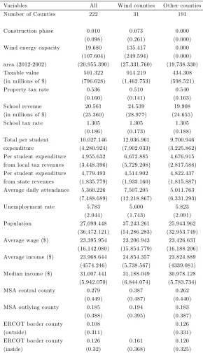
Table 2: Regression variables
Variables All Wind counties Other counties Number of Counties 222 31 191
Construction phase 0.010 0.073 0.000 (0.098) (0.261) (0.000) Wind energy capacity 19.680 135.417 0.000
(107.604) (249.594) (0.000) area (2012-2002) (20,955.390) (27,331.760) (19,738.330) Taxable value 501.322 914.219 434.308 (in millions of $) (796.628) (1,462.753) (598.521) Property tax rate 0.536 0.510 0.540
(0.160) (0.141) (0.163) School revenue 20.561 24.539 19.908 (in millions of $) (25.360) (28.977) (24.655) School tax rate 1.305 1.305 1.305
(0.186) (0.173) (0.188) Total per student 10,027.146 12,036.961 9,700.946 expenditure (4,280.924) (7,902.033) (3,225.862) Per student expenditure 4,955.632 6,672.885 4,676.915 from local tax revenues (3,448.396) (5,729.208) (2,817.588) Per student expenditure 4,779.493 4,514.902 4,822.437 from state revenues (1,835.779) (1,933.160) (1,815.887) Average daily attendance 5,360.226 7,507.205 5,011.763
(7,488.689) (12,218.867) (6,331.293) Unemployment rate 5.783 5.600 5.823
(2.044) (1.743) (2.091) Population 27,099.448 37,243.261 25,943.962
(36,472.121) (54,286.283) (32,953.749) Average wage ($) 23,395.954 23,206.943 23,426.631
(16,142.080) (15,854.779) (16,188.206) Average income ($) 23,968.644 24,854.357 23,824.889
(4574.246) (5,738.567) (4339.081) Median income ($) 31,007.441 31,188.049 30,978.128 (5,942.070) (6,844.074) (5,783.734) MSA central county 0.279 0.387 0.262
(0.449) (0.487) (0.440) MSA outlying county 0.185 0.194 0.183
at the the beginning of the study period. Since wind development has taken place in the relatively
rural counties, it would be innappropriate to compare outcomes between the relatively static rural
counties and the urban counties that have enjoyed substantial population and employment growth
over the period from factors unrelated to wind power. Speci…cally, we exclude counties with
popu-lations less than 421 or greater than 200,347 in 2001 (the largest wind county by population) or per
capita personal income less than $13,865 or greater than $30,804 in 2001 (the highest value among
the wind counties). This restriction reduces the number of counties used in the anlaysis from 254 to
222. The excluded counties are the more populous counties found along the I-35 corridor (the
Dallas-Fort Worth, Austin/San Antonio, and Houston metropolitan areas), the (Rio Grande) Valley region
of Texas, El Paso, Lubbock, and Midland. Only one county, Loving County, with a 2001 population
of 72, failed to meet the minimum values.24
Table 1 presents two-digit NAICS industry-level data on numbers of estalishments and employment
levels for the wind and non-wind counties in Texas. For each subset, the table includes both average
values over the eleven years of observations and the average changes in total values between the two
sample years of 2001 and 2011.
Comparisons between wind counties and non-wind counties at the beginning of the study period
are clearer when looking at Table 2. One observes that wind counties, on average, are more populous
than control counties. Wind counties have only a slightly higher number of establishments and
employees than the average control county. The largest disparities are in the wholesale, retail, scienti…c,
transportation, and health sectors. Average income and wages are the same in both, for practical
purposes. However, there are contrasting di¤erences in the values of the property tax bases and
school revenues, as would be expected from the di¤erences in average county populations. Average
taxable value and school revenues are higher by about $500 million and $5 million respectively in the
wind counties compared to non-wind counties. Not surprisingly, wind counties’ average daily school
attendance is higher by about 2,500 pupils compared to the other counties in the analysis. Finally,
average wind generation capacity in wind counties is about 135 MW.
Panel A in Figure 1 represents the distribution of wind generation capacity in 2001. In total,
Figure 1: Wind energy generation counties in Texas
Panel A: Wind energy capacity in 2001
Figure 2: Taxable value, property tax rate, school tax rate, and wind energy capacity
there were only 6 counties with about 900 MW in total capacity. In Panel B we show wind generation
capacity by county in 2012. As can be seen, it has increased to 32 counties with total capacity in excess
of 12,000 MW. In Figure 2, we show some summary plots depicting the relationship between taxable
property value, wind capacity, and property tax rates in the top two panels and school revenues, school
tax rates, and wind capacity in the bottom two panels. We see that total taxable property value is
increasing in wind generation capacity while property tax rates (and school tax rates) are decreasing in
wind energy generation capacity. However, one should be cautious in interpreting these observations
as they are summary plots.25
3.2
Empirical Analysis
3.2.1 Industry E¤ects
We …rst investigate the impact of wind development on levels of establishments and employment in
each county. We look at the 10-year change in both the numbers of establishments and employed
persons between 2001 and 2011 in the subset of all wind and non-wind energy generation counties in
Texas, as described above. We regress these changes on, inter alia, the changes in installed wind
power capacity between 2001 and 2011. The model to be estimated is as follows:
yc;T t1 = 0+ 1 wc;T t1+x
0
c;t1 +z
0
c;j;t1 +m
0
c +"c (1)
Our dependent variable (y) is either the di¤erence in number of establishments or employees between
2001 and 2011 per county. Our independent variables can be categorized into four groups: county-level
wind capacity in 100 MW units (w), county characteristics that vary with time such as unemployment
rate and population, (x) industry characteristics such as industry speci…c county-level wages (z), and
county characteristics that do not vary with time such as MSA central or peripheral county (m). The
term"c;j is the error.
Table 3 contains the OLS estimation results from three speci…cations for both of the outcome
vari-ables. As can be seen, the estimated coe¢cient for the change in total county wind capacity is positive
but statistically insigni…cant for both establishments and employment in all speci…cations. While a
…nding of no statistical evidence of an employment impact is contrary to our initial expectations, given
the results from the other studies surveyed, it should perhaps not be too surprising in Texas. For
Table 3: Regression results for 10 year change in number of establishments and employees
Variables Number of …rmsc;T10 t1 Number of employeesc;T10 t1
(1) (2) (3) (4) (5) (6) Wind energy 1.861 1.619 3.031 115.519 112.102 118.219 capacityc;T10 t1 (in 100 MW) (11.087) (5.485) (5.309) (127.312) (77.989) (73.078)
Unemployment ratec;t1 -6.290 -5.780 34.937 38.372
(4.990) (4.842) (107.455) (112.598) Populationc;t1 0.010*** 0.010*** 0.103*** 0.110***
(0.001) (0.001) (0.018) (0.021) Wagesc;t1(in $10,000) 0.000 0.001 -0.012 0.004
(0.001) (0.001) (0.032) (0.029) MSA central countyc -63.600** -1,066.514
(25.802) (672.342) MSA outlying countyc -12.287 215.300
(20.363) (408.231) ERCOT border county -36.026 -1,107.415
(outside)c (29.076) (796.311)
ERCOT border county 3.680 -727.409
(inside)c (24.346) (608.696)
Observations 222 222 222 222 222 222 R2 0.000 0.868 0.872 0.002 0.562 0.576 Robust standard errors in parentheses
the average total wind plant of 135 MW, in the wind counties, a sizeable employment impact of .482
jobs/MW implies an average employment increase of 65 jobs, or only about 0.05% of the average wind
county employment of 13,653. Such a small proportional change is di¢cult to discern statistically.
In order to consider the possibility of e¤ects within and across industries, that may tend to o¤set
one another, we disaggregate county employment in Texas using both establishment and employment
data by industry for the 10 year change within the 20 industrial categories of the NAICS-2 in the
QCEW as reported by the Texas Workforce Commission. Analysis at the NAICS-2 industry-level
should provide greater statistical precision in estimating changes in establishments or employment
than the estimate of changes in total (all industries) outcomes if any changes are concentrated in a
subset of industries and/or opposite in sign. As noted, we are aware of the changes to the NAICS
industrial categories that occurred during the course of the decade but proceed under the view that
substantive changes at the NAICS-2 level of aggregation are insigni…cant.
By considering the 10-year change, our goal is to observe persistent e¤ects and to avoid transient
construction impacts at the industry level. At least for direct employment measures, this should not
pose an issue, even for 2011. Since the QCEW data are establishment-based, and given that the
bulk of the construction activity relies on specialized construction …rms, and few of these …rms are
local establishments, the recorded construction employment e¤ects would largely be associated with
the external locality in which the employing establishments are located.
We again specify two models for each outcome variable. Similar to total employment, the observed
di¤erences in the industry-level outcome variables between 2001 and 2011 are regressed,inter alia, on
the total change in wind power capacity in each county during the period 2001-2011. We consider the
following empirical model:
yc;j;T t1 = 0+ 1 wc;T t1+x
0
c;t1'+z
0
c;j;t1 +m
0
c#+ c;j (2)
Our dependent variable (y) is either the di¤erence in number of establishments or employees in industry
j between 2001 and 2011 by NAICS-2 per county. Independent variables are similar to the ones
described in equation 1. The term c;j is the error.
Table 4 contains regression results for di¤erences in the number of establishments across the 20
Table 4: Regression results for 10 year change in number of establishments
Panel A
Variables Number of …rmsc;j;T10 t1
Agriculture Mining Utilities Construct. Manufact. Wholesale Retail Transport Information Finance
Wind energy -0.365* 0.903** 0.143* 0.308 0.035 -0.081 0.263 0.594 0.155 0.457
capacityc;T10 t1 (in 100 MW) (0.216) (0.415) (0.076) (1.134) (0.190) (0.664) (0.605) (0.756) (0.140) (0.432)
Unemployment ratec;t1 -0.064 -0.626* -0.185** -1.478* -0.131 -0.266 -0.220 -0.087 -0.015 -0.232
(0.470) (0.330) (0.074) (0.819) (0.204) (0.335) (0.662) (0.490) (0.091) (0.302)
Populationc;t1 -0.000 0.000*** 0.000*** 0.002*** 0.000*** 0.001*** 0.001*** 0.001** 0.000*** 0.001***
(0.000) (0.000) (0.000) (0.000) (0.000) (0.000) (0.000) (0.000) (0.000) (0.000)
Wagesc;t1(in $10,000) 0.000 0.000 0.000 0.001* 0.000*** 0.000 -0.000 -0.000 0.000 0.000
(0.000) (0.000) (0.000) (0.000) (0.000) (0.000) (0.000) (0.000) (0.000) (0.000)
MSA central countyc 4.781 -1.376 1.216** -5.087 -1.429 -6.069** -9.254** -11.680 -0.643 -2.559
(3.501) (2.800) (0.563) (7.533) (1.865) (2.634) (3.772) (9.541) (0.765) (2.039)
MSA outlying countyc -0.819 -1.467 -0.419 4.981 1.954 -0.473 -0.723 -3.754 -0.353 -3.599**
(2.156) (2.280) (0.556) (4.581) (1.699) (2.387) (2.658) (4.424) (0.590) (1.669)
ERCOT border county 3.953 -0.498 0.386 -13.012*** -2.051 -2.283 -6.071** -4.780 0.506 -0.111
(outside)c (4.460) (3.831) (0.666) (4.752) (2.662) (2.796) (2.717) (3.398) (0.713) (2.891)
ERCOT border county -0.062 0.659 -0.473 -5.750 -1.500 0.931 -1.003 -1.414 0.499 -1.184
(inside)c (3.171) (2.830) (0.379) (3.578) (1.420) (1.972) (2.610) (3.106) (0.763) (2.073)
Observations 222 222 222 222 222 222 222 222 222 222
R2 0.037 0.325 0.324 0.833 0.505 0.714 0.821 0.453 0.735 0.845
Panel B
Real Estate Scienti…c Manag. Waste Mng. Education Health Care Arts Ent Accommod. Other Public adm.
Wind energy 0.183 0.701 -0.001 0.142 -0.017 0.302 0.196 -0.248 0.220 -0.329
capacityc;T10 t1 (in 100 MW) (0.271) (1.030) (0.065) (0.399) (0.116) (0.812) (0.120) (1.046) (0.714) (0.241)
Unemployment ratec;t1 -0.030 -0.484 -0.077 -0.098 0.054 -0.782 -0.165 -0.242 -1.136 -0.346
(0.367) (0.801) (0.054) (0.286) (0.139) (0.559) (0.143) (1.251) (0.749) (0.218)
Populationc;t1 0.000*** 0.001*** 0.000*** 0.001*** 0.000*** 0.001*** 0.000*** 0.001** 0.001*** 0.000***
(0.000) (0.000) (0.000) (0.000) (0.000) (0.000) (0.000) (0.000) (0.000) (0.000)
Wagesc;t1(in $10,000) 0.000 0.000 -0.000 0.000* 0.000 -0.000 0.000 -0.001 0.000 0.000***
(0.000) (0.000) (0.000) (0.000) (0.000) (0.000) (0.000) (0.001) (0.000) (0.000)
MSA central countyc -1.190 -9.251** 0.060 -2.817 0.706 -6.370* 0.754 -4.199 -10.268* -1.079
(1.800) (3.611) (0.494) (2.195) (1.009) (3.319) (0.820) (7.830) (5.626) (1.763)
MSA outlying countyc -1.730 -0.418 -0.559* 1.150 0.576 -1.348 0.278 -6.017 -5.693* 0.097
(1.245) (3.449) (0.289) (1.753) (0.724) (2.301) (0.606) (5.993) (3.320) (1.223)
ERCOT border county -1.869 -4.125 0.060 -0.512 0.585 -5.120 -1.348* 6.797 -7.028* -1.930
(outside)c (1.551) (3.315) (0.453) (2.399) (0.617) (3.240) (0.739) (6.827) (3.800) (2.203)
ERCOT border county -1.034 0.917 0.392 -0.394 -0.223 0.577 -1.084** 10.921** 3.135 -2.148*
(inside)c (1.202) (3.785) (0.469) (1.777) (0.588) (2.815) (0.455) (4.925) (8.689) (1.258)
Observations 222 222 222 222 222 222 222 222 222 222
R2 0.753 0.751 0.500 0.812 0.640 0.872 0.621 0.140 0.781 0.548
Table 5: Regression results for 10 year change in number of employees
Panel A
Variables Number of employeesc;j;T10 t1
Agriculture Mining Utilities Construct. Manufact. Wholesale Retail Transport Information Finance
Wind energy -11.991 10.745 0.393 22.235 24.455 -2.492 19.845* -10.191 -2.517 9.228
capacityc;T10 t1 (in 100 MW) (8.993) (17.920) (1.879) (17.125) (16.294) (6.476) (11.589) (11.480) (4.095) (8.583)
Unemployment ratec;t1 4.653 -15.038 0.209 -10.545 -6.563 -3.366 -9.828 2.130 -1.034 2.523
(5.003) (10.779) (1.868) (8.373) (31.938) (6.654) (22.942) (8.607) (2.122) (5.600)
Populationc;t1 -0.001 0.008*** 0.001** 0.016*** -0.009 0.004*** 0.010*** 0.008*** 0.000 0.000
(0.001) (0.002) (0.000) (0.003) (0.007) (0.001) (0.003) (0.002) (0.001) (0.001)
Wagesc;t1(in $10,000) -0.001 0.003 0.001 0.009* 0.019* -0.001 -0.001 -0.005 -0.001 0.002
(0.001) (0.004) (0.001) (0.006) (0.011) (0.003) (0.005) (0.003) (0.001) (0.002)
MSA central countyc 21.383 7.154 23.646 63.834 -22.482 53.002 -131.107 -40.604 -27.832 41.920
(32.671) (103.892) (15.442) (99.436) (245.618) (64.165) (134.827) (74.383) (18.264) (40.974)
MSA outlying countyc 0.999 -40.809 -4.998 -106.422 398.620** 40.415 51.022 1.957 11.164 17.214
(23.822) (88.297) (17.455) (69.596) (185.665) (48.827) (65.718) (43.960) (14.856) (31.635)
ERCOT border county -13.362 -21.620 -0.825 115.432 -409.883 -120.393 -189.059*** -20.064 -15.532 -94.410
(outside)c (45.383) (117.407) (11.671) (216.163) (473.481) (118.231) (70.808) (67.891) (35.142) (78.729)
ERCOT border county -28.747 -39.357 28.258* -70.105 -379.512 -13.032 -445.404* 1.036 20.374 -24.914
(inside)c (30.375) (74.532) (15.043) (48.123) (352.441) (27.948) (246.790) (42.778) (24.993) (18.464)
Observations 222 222 222 222 222 222 222 222 222 222
R2 0.041 0.197 0.152 0.569 0.081 0.178 0.224 0.410 0.013 0.048
Panel B
Real Estate Scienti…c Manag. Waste Mng. Education Health Care Arts Ent Accommod. Other Public adm.
Wind energy 1.813 4.345 -0.837 20.996* 11.430 1.691 -2.284 8.172 2.123 8.900
capacityc;T10 t1 (in 100 MW) (1.455) (8.290) (1.488) (10.955) (38.952) (15.957) (2.191) (19.678) (5.204) (15.605)
Unemployment ratec;t1 -0.194 -5.401 -2.009 6.826 98.589 -6.978 0.747 3.503 -3.404 -5.254
(2.861) (4.682) (2.153) (12.946) (70.491) (15.348) (2.318) (22.744) (4.322) (10.535)
Populationc;t1 0.002*** 0.006*** 0.001*** 0.005 0.049*** 0.015*** 0.001*** 0.004 0.004*** 0.006***
(0.001) (0.001) (0.000) (0.004) (0.013) (0.005) (0.000) (0.004) (0.001) (0.002)
Wagesc;t1(in $10,000) 0.001 -0.001 0.000 0.004 0.000 -0.008 -0.001 -0.014 0.002 0.001
(0.001) (0.002) (0.001) (0.007) (0.010) (0.008) (0.001) (0.011) (0.001) (0.006)
MSA central countyc -9.713 -47.945 -0.571 -34.347 -547.015 -163.997 12.148 -85.887 -5.713 -61.577
(19.995) (29.455) (15.192) (69.059) (357.832) (179.504) (15.197) (137.390) (30.207) (107.259)
MSA outlying countyc -16.231 -19.317 -23.667** -23.781 -163.173 139.894 -3.334 -75.994 -13.273 -26.263
(11.022) (21.991) (9.758) (51.684) (194.221) (103.437) (8.950) (99.902) (17.882) (47.950)
ERCOT border county -1.775 7.820 11.959 34.769 -84.912 -381.140 -17.856* 120.638 -10.049 134.082
(outside)c (19.224) (44.535) (19.540) (56.626) (174.068) (292.482) (9.543) (114.166) (22.098) (168.416)
ERCOT border county -6.190 7.788 24.260 65.242 -72.292 99.695 -3.005 199.776** -0.697 -49.852
(inside)c (12.040) (31.593) (19.795) (55.554) (171.673) (102.199) (8.686) (98.784) (30.044) (54.857)
Observations 222 222 222 222 222 222 222 222 222 222
that occurred over the decade. Consistent with the substitution in land-use that wind power implies,
the e¤ect on the number of agricultural establishments is negative.26
Table 5 considers the decade change in growth of total employment by industry, a more interesting
comparison than establishments. Only employment in retail and waste management appears to have
been positively a¤ected by wind development. Although statistical signi…cance is low, these estimates
suggest a total indirect/induced e¤ect in these two industries of about 40 jobs per 100 MW. Increases
in local retail activity would be expected through higher levels of spending associated with higher
levels of personal income from wind power production, a so-called induced e¤ect. Waste management
employment would be a¤ected by the need for services in the recycling and disposal of turbine
lubri-cating oil, hydraulic and cleaning ‡uids. Although the number of agricultural establishments declines
with wind power development, there is no evidence of such a change in employment in agricultural
industry activities. It is worth noting at this point that employment in education shows no e¤ect,
suggesting that any localized property and school tax bene…ts from the increase in …xed wind plant
did not result in measurable increases in school employment. Nor is there any statistically signi…cant
change in employment in the utilities sector.
While this latter result is surprising, a look at unconditional comparisons helps to provide credibility.
There were positive changes of about 14.0 jobs in utilities employment in the control counties, and 15.8
in the wind counties. Based on this unconditional, and relatively simple, comparison, the di¤erence of
fewer than two jobs (less than 2 percent of total industry employment) between the changes in average
utilities employment between the control and the wind counties is not great enough to infer a clear
statistical di¤erence.
One caveat may be in order. Since the QCEW employment data are establishment-based, if on-site
turbine O&M personnel are employed and reported by an establishment, either the plant operator or
a relevant sub-contractor, that is located in another county (or state), then those jobs will not appear
in our employment data for the given wind county. Remote monitoring and operation of turbines
can take place from anywhere on the globe. If, for example, oil temperatures increased slightly, the
turbine can be remotely shut down and a technician dispatched from a regional o¢ce to look into
the situation. Moreover, this technician may be employed by a sub-contractor in an establishment
which does not report under NAICS 22. Indeed, when looking at fully disclosed establishment-based
QCEW data for Texas up to 2006, we cannot locate the great majority of wind plants in the counties
where those wind plants are known to be sited. However, we do …nd establishment-based employment
for wind generation …rms (searching at the NAICS-6 level) in Austin and Houston, areas with no
installed utility-scale wind plant. This suggests that direct employment e¤ects may rather be found in
establishments that report employment in regional population hubs or remote cities where wind plant
operators base their administrative operations.
While we …nd positive e¤ects from wind development on employment levels at the industry level,
these e¤ects have to be interpreted in the context of the result that there was no signi…cant
wind-related change in total county employment levels. These conclusions are not inconsistent if there have
been small, o¤setting changes in other industrial employment that were below the level of statistical
detection. Thus, we believe that employment gains related to wind development have tended to crowd
out employment in other activities, indicating that labor has been inelastically supplied in these rural
counties.
3.2.2 County Personal Income
We next turn our attention to the relationship between income and wind energy development. However,
we must …rst investigate the question of endogeneity between wind development and county income.
It may be that an endogenous relationship exists because, for example, higher income in a county
re‡ects a higher level of …nancial or business acumen. Such a county may be better positioned to
establish relationships with wind energy developers and increase the likelihood that wind development
will occur. On the other hand, given the environmental issues surrounding the siting of wind plant,
lower income counties may be more receptive or more likely to seek out wind development. If the initial
income level is signi…cant in explaining growth in income up to 2011, i.e., regression toward the mean
suggests that counties with lower initial income would grow faster than counties with higher initial
income, then income changes could be erroneously attributed to wind development if a signi…cant
correlation between wind development and initial income exists. We empirically examine this question
by estimating whether or not initial or year 2001 county characteristics (x) that are unrelated to wind
period. Note that in year 2001, there were only 6 counties producing wind energy with total capacity
of less than 900 MW.
Our empirical model is presented in equation 3. Here, the dependent variable is the level of wind
capacity in year 2011. Initial conditions (2001) such as per capita income, unemployment rates, and
population are represented in the matrix (x) and county characteristics that do not change over time
are represented in matrix (m). The variables that do not change over time are modeled by dummy
variables. There is a dummy that captures whether the county is in the ERCOT area (1) or not (0), two dummies to identify if the county is a central or peripheral MSA county, and another dummy for
the 178 counties with an average wind resource categorized as Class 2 or higher.27
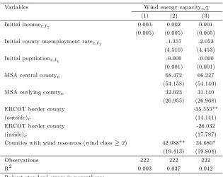
wc;T = 0+x0c;t=1&+m0c'+ c (3)
Our results in Table 6 indicate that initial per capita income is not an explanatory factor in the
choice of a speci…c county for wind farm location. Not surprisingly, the coe¢cient of the “wind
resources” dummy appears to provide all the explanatory power. The presence of the wind resource is
exogenous to county location and unchanged over the period of this analysis.
Given this result, OLS will provide an unbiased means to estimate the e¤ect of installed wind
generation capacity on county-level per capita income. To examine this e¤ect, we estimate county-level
per capita income as function of installed wind capacity controlling for observable and unobservable
county and time e¤ects. Note that the empirical approach will capture net changes to county per
capita income due to wind development, i.e., wind power-related changes net of displaced agricultural
and other industrial activity-related changes.
Consider the following empirical model:
Ic;T t1 = c+ (w=pop)c;T t1+'unempc;t1+x
0
c;t 1 + c;t (4)
Depending on the speci…cation, the dependent variable is either the change in level of county per capita
income or county median income between 2000 and 2011. Thus, the regression captures a one-time
Table 6: Regression results for wind installation capacity
Variables Wind energy capacityc;T
(1) (2) (3) Initial incomec;t1 0.003 0.002 0.001
(0.005) (0.005) (0.005) Initial county unemployment ratec;t1 -1.357 -2.053
(4.510) (4.453) Initial populationc;t1 -0.000 -0.000
(0.001) (0.001) MSA central countyc 68.472 66.227
(54.158) (54.140) MSA outlying countyc 32.023 31.140
(26.955) (26.968) ERCOT border county -35.555**
(outside)c (14.141)
ERCOT border county -26.032
(inside)c (17.787)
Counties with wind resources (wind class 2) 42.088** 34.680* (19.413) (19.804)
Observations 222 222 222
R2 0.003 0.037 0.042
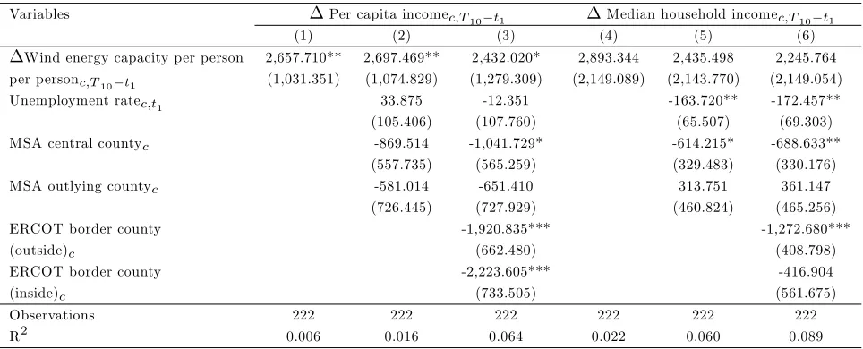
Table 7: Regression results for income
Variables Per capita incomec;T10 t1 Median household incomec;T10 t1
(1) (2) (3) (4) (5) (6)
Wind energy capacity per person 2,657.710** 2,697.469** 2,432.020* 2,893.344 2,435.498 2,245.764 per personc;T10 t1 (1,031.351) (1,074.829) (1,279.309) (2,149.089) (2,143.770) (2,149.054)
Unemployment ratec;t1 33.875 -12.351 -163.720** -172.457**
(105.406) (107.760) (65.507) (69.303) MSA central countyc -869.514 -1,041.729* -614.215* -688.633**
(557.735) (565.259) (329.483) (330.176) MSA outlying countyc -581.014 -651.410 313.751 361.147
(726.445) (727.929) (460.824) (465.256) ERCOT border county -1,920.835*** -1,272.680***
(outside)c (662.480) (408.798)
ERCOT border county -2,223.605*** -416.904
(inside)c (733.505) (561.675)
Observations 222 222 222 222 222 222
R2 0.006 0.016 0.064 0.022 0.060 0.089
Robust standard errors clusterd by counties in parentheses. *** p<0.01, ** p<0.05, * p<0.1
change in per capita personal income or median income between 2001 and 2011 as a function of the
total of all increments in county wind capacity between 2001 and 2011. The wind capacity variable is
measured as MW per person. Results are presented in Table 7.
Considering the e¤ects of changes in installed wind capacity on per capita county income, the value
of the estimated coe¢cient, while large, is quite reasonable within the estimation context. Using the
average population for wind counties of 37,243 persons, a 100 MW increase in wind capacity would
imply an increase in county per capita income of about $7.13 in base year dollars or .03 per cent.
That then implies an increase in average county total income of $2,657 per installed MW. For a small
population county, such as Sterling County, population 1,158 in 2011, a 100 MW plant would generate
an increase in per capita personal income of $230 in year 2000 dollars. Considering the example of the
662.5 MW Capricorn Ridge installation in Coke and Sterling Counties, combined population of 4,463
in 2011, our results suggest an increase of $395 in per capita income across the two counties, which
represents an increase on the order of 2 percent (based on a weighted average per capita income in
2001 of $19,537).
Columns 4-6 contain the coe¢cient estimates for the model with the change in median county