arXiv:1511.04387v2 [cs.DS] 8 Sep 2016
Combining Monte-Carlo and Hyper-heuristic methods for the
Multi-mode Resource-constrained Multi-project Scheduling
Problem
Shahriar Astaa, Daniel Karapetyana,b,∗, Ahmed Kheiria, Ender ¨Ozcana,
Andrew J. Parkesa
a
University of Nottingham, School of Computer Science Jubilee Campus, Wollaton Road, Nottingham, NG8 1BB, UK b
University of Essex, Institute for Analytics and Data Science Wivenhoe Park, Colchester, CO4 3SQ, UK
Abstract
Multi-mode resource and precedence-constrained project scheduling is a well-known challenging real-world optimisation problem. An important variant of the problem re-quires scheduling of activities for multiple projects considering availability of local and global resources while respecting a range of constraints. A critical aspect of the bench-marks addressed in this paper is that the primary objective is to minimise the sum of the project completion times, with the usual makespan minimisation as a secondary objective. We observe that this leads to an expected different overall structure of good solutions and discuss the effects this has on the algorithm design. This paper presents a carefully designed hybrid of Monte-Carlo tree search, novel neighbourhood moves, memetic algo-rithms, and hyper-heuristic methods. The implementation is also engineered to increase the speed with which iterations are performed, and to exploit the computing power of multicore machines. Empirical evaluation shows that the resulting information-sharing multi-component algorithm significantly outperforms other solvers on a set of “hidden” instances, i.e. instances not available at the algorithm design phase.
Keywords: metaheuristics; hybrid heuristics; hyper-heuristics; Monte Carlo tree search; permutation based local search; multi-project scheduling
1. Introduction
Project scheduling has been of long-standing interest to academics as well as prac-titioners. Solving such a problem requires scheduling of interrelated activities (jobs), potentially each using or sharing scarce resources, subject to a set of constraints, and with one or several of a variety of objective functions. There are various project schedul-ing problems and many relevant surveys in the literature, e.g. see [4, 22, 21, 48, 39, 20, 65]. The best-known problem class is the Resource Constrained Project Scheduling Problem
∗Corresponding author
(RCPSP) in which activities have fixed usages of the resources, there are fixed prece-dence constraints between them, and often the objective is simple minimisation of the makespan (completion time of last activity). These problems have been proven to be NP-hard [2], and a well-known benchmark suite, PSPLIB, is provided in [29].
A generalisation of the RCPSP is to also consider ‘Multi-mode RCPSP’ (MRCPSP) in which activities can be undertaken in one of a set of modes, with each mode potentially using different sets of resources. Furthermore, there are many options besides makespan for the objective function(s); a typical one is that a weighted sum of completion times is minimised. As common in optimisation problems, exact methods perform best on smaller instances and on larger instances heuristics and metaheuristics become necessary. Recent works on the MRCPSP range from exact approaches, such as, MILP [33], and branch-and-bound [59], to metaheuristics, such as, differential evolution [11], estimation of distribution algorithms [61], evolutionary algorithms [14, 55, 17], swarm intelligence methods [31], and others [8, 60].
This paper presents our winning approach submitted to MISTA 2013 challenge1on a
further extension called ‘multi-mode resource-constrained multi-project scheduling’ (MR-CMPSP) and the results on the associated benchmark/competition instances. The full description of this problem domain can be found on the competition website and in [62]; however, for completeness we also summarise it in Section 2. The broad aim is to schedule a set of different and partially interacting projects, with each project consist-ing of a set of activities. There are no precedence constraints between the activities of different projects however they can compete for resources. Also, the objective function is extended to be a mix of a kind of weighted completion time and makespan. The MRCMPSP is hence interesting in that it has a mix of structures and requirements that are a step towards modelling the complexity of real-world scheduling problems. The high real-world relevance of the multi-project version of scheduling is well-known, e.g. a survey [35] found that “84% of the companies which responded to the survey indicated that they worked with multiple projects”. However, the majority of scheduling work is on the single project version, though there is some existing work on the multi-project case, e.g. see [35, 18, 32, 36].
Our approach searches the space of sequences of activities, from which schedules are constructed and then the quality of each schedule is evaluated using the objective func-tion. The search process on the set of sequences operates in two phases in a “construct and improve” fashion. In the first phase, a heuristic constructor creates initial sequences of activities. A novel proposal in this paper is to investigate the overall global structure of the solutions and use this to motivate constructing the initial sequences using a Monte-Carlo Tree Search (MCTS) method, e.g. see [3]. This construction phase is followed by an improvement phase which makes use of a large and diverse set of heuristic neighbour-hood moves. The search process during the improvement phase is carefully controlled by a combination of methods arising from a standard metaheuristic, namely memetic algorithm, and also an extension of existing hyper-heuristic components [27, 46].
There is an interesting potential for dual views of the overall problem. It is defined as a multi-project problem, but it can be also viewed as a single project (multi-mode) RCPSP, in which the precedence graph has a particular structure, consisting of disjoint clusters.
1
There is a sense in which we work with both views together. Some neighbourhood moves treat the problem in a single-project fashion and work on the constituent activities; other neighbourhood operators explicitly consider the multi-project nature of the problem, and focus on moves of projects. Both views, and kinds of operators, are used and work together to improve the overall project-level structure as well as the detailed activity level structure. A discussion and a computational study on both approaches can be found in [35].
The primary contributions of this paper are:
• Observation and investigation of how the primary objective function being essen-tially a “sum of project completion times” leads to good solutions having inherently different structure to those with makespan as the primary objective. In particular, minimisation of project completion times subject to limited global resource results in partial ordering of projects; this does somewhat reduce the effective size of the search space, but also may lead to good solutions being more widely separated. Un-derstanding of this significantly affected our algorithm design, including an MCTS construction method aiming to create solutions having such structure.
• Novel neighbourhood moves, including those that are designed specifically for smoother navigation through the search space of the multi-project extension of MRCPSP – reflecting our observation of the effect that the main objective func-tion has on the solufunc-tion structures.
• An adaptive hybrid hyper-heuristic system to effectively control the usage of the rich set of neighbourhood moves.
• Evidence of the effectiveness based on successful results on a range of benchmark problems. This includes winning a competition, in which some problems were hidden at the algorithm design/tuning phase. We also tested our algorithm on single-project instances from PSPLIB. Although our algorithm was not designed to work on single-project instances, it demonstrated good performance in these tests, and was competitive with the state-of-the-art methods tailored to the single-project case. Furthermore, it improved 3 best solutions on these PSPLIB instances during these experiments.
These contributions are directed towards a system that is both robust and flexible; with the potential to be effective at handling a wide variety of problem requirements and instances. Arguably, one of the lessons of this paper is that greater complexity and richness of such scheduling problems needs to be matched with a greater complexity and richness of the associated algorithms; especially when not all instances are known in advance, and so algorithms should not over-specialise to a particular data set.
Regarding the structure of the paper; in Section 2 we describe the problem to be solved. In Section 3 we discuss how we have carefully chosen the appropriate data struc-tures and implemented algorithms operating with those data strucstruc-tures efficiently in order to construct the schedule from a given sequence as fast as possible. (To build an effective system, one has to pay attention to all of its components.) However, most of the contribution of this paper arises from choosing and combining the effective algo-rithmic components including the search control algorithm and then (partially) tuning the relevant parameters within the overall approach. These consist of the MCTS-based
constructor given in Section 4, the neighbourhoods given in Section 5, and the improve-ment phase given in Section 6. The computational experiimprove-ments and competition results are presented and analysed in Section 7; including some reports of performance on a multi-mode, though single project, benchmark set from PSPLIB. Section 8 concludes the paper.
2. Problem Description
The problem consists of a setP ofprojects, where each projectp∈P is composed of a set of activities, denoted as Ap, a partition from all activities A. Each projectp∈P
has a release time ep, which is the earliest start time for the activitiesAp.
The activities are interrelated by two different types of constraints: the precedence constraints, which force each activity j ∈ A to be scheduled to start no earlier than all the immediate predecessor activities in set Pred(j) are completed; and the resource constraints, in which the processing of the activities is subject to the availability of resources with limited capacities. There are three different types of the resources: local renewable, local non-renewable and global renewable. Renewable resources (denoted using the superscript ρ) have a fixed capacity per time unit. Non-renewable resources (denoted using the superscriptν) have a fixed capacity for the whole project duration. Global renewable resources are shared between all the projects while local resources are specified independently for each project.
Renewable and non-renewable resources are denoted using the superscript ρand ν, respectively. Rρ
p is the set of local renewable resources associated with a projectp∈P,
and Rρpk is thecapacity of k ∈Rρ
p, i.e. the amount of the resourcek available at each
time unit. Rν
p is the set of local non-renewable resources associated with a projectp∈P,
and Rν
pk is the capacity of k ∈Rpν, i.e. the amount of the resource k available for the
whole duration of the project. Gρ is the set of the global renewable resources, andGρ k is
the capacity of the resourcek∈Gρ.
Each activityj∈Ap,p∈P, has a set of execution modes Mj. Each modem∈Mj
determines the duration of the activitydjm and the activity resource consumptions. For
a local renewable resource k ∈Rρ
p, the resource consumption is r ρ
jkm; for a local
non-renewable resource k ∈ Rν
p, the resource consumption is rjkmν ; for a global renewable
resourcesk∈Gρ, the resource consumption isgρ
jkm.
Schedule D = (T, M) is a pair of time and mode vectors, each of size n. For an activity j ∈ A, valuesTj and Mj indicate the start time and the execution mode of j,
respectively. ScheduleD= (T, M) is feasible if:
• For eachp∈P and eachj∈Ap, the project release time is respected: Tj≥ep;
• For each project p∈P and each local non-renewable resource k∈ Rν
p, the total
resource consumption does not exceed its capacityRν pk.
• For each projectp∈P, each time unittand each local renewable resourcek∈Rρ
p,
the total resource consumption attdoes not exceed the resource capacityRρpk.
• For each time unittand each global renewable resourcek∈Gρ
p, the total resource
• For eachj ∈A, the precedence constraints hold: Tj ≥maxj′∈Prec(j)Tj′ +dj′Mj′.
The objective of the problem is to find a feasible schedule D = (T, M) such that it minimises the so-called total project delay (TPD), defined by using the time for total project completion (TPC)
TPC =X
p∈P
Cp (1)
and
TPD≡fd(D) = TPC−L=
X
p∈P
Cp
−L , (2)
whereCp is the completion time of projectp
Cp= max j∈Ap
Tj+djMj
. (3)
The constantLis a lower bound calculated as
L=X
p∈P
(CPDp+ep), (4)
with CPDp being a given pre-calculated value. Since L is a constant, then it does not
affect the optimisation (it was presumably introduced in the competition just to make the output numbers smaller and easier to interpret). Specifically, since L is the lower bound (though not necessarily a tight bound), fd(D)≥0 for any feasible solutionD.
Note that this primary objective is an instance of the standard “weighted completion time”, usually denoted by “P
jwjCj”, but specialised to the case, “PpwpCp”, in which
only the completion times of the projects are used2 (in the case of TPD all the weights
are assigned to be one).
The tie-breaking secondary objective is to minimise thetotal makespan, (TMS), which is the finishing time of the last activity (or equivalently of the last project):
TMS≡fm(D) = max
j∈A Tj+djMj
= max
p∈P Cp. (5)
In our implementation, we combine the objective functions fd(D) and fm(D) into
one function f(D) that gives the necessary ranking to the solutions:
f(D) =fd(D) +γfm(D), (6)
where 0< γ≪1 is a constant selected so thatγfm(D)<1 for any solutionDproduced
by the algorithm. In fact, we sometimes use γ= 0 to disable the second objective. For details, see Section 6.1.
Under the conventional “α|β|γ” labelling, it could perhaps be described as “MP+S|
prec |(P
pwpCp, Cmax)” using ‘MP+S’ to denote ‘Multi-mode Multi-Project
Schedul-ing’.
2
If there is no unique activity marking the end of a project, then a dummy empty end activity can always be added, without changing the problem.
3. Schedule Generator
Designing an algorithm for solving the multi-mode resource-constrained multi-project scheduling problem requires an appropriate solution representation. There are two ‘nat-ural’ solution representations in the scientific literature:
Schedule-based: A direct representation using the assignment times, and also modes, of activities, i.e. vectorsT andM.
Sequence-based: This is based on selecting a total order on all the activities. Given such a sequence, a time schedule is constructed by taking the activities one at a time in the order of the sequence and placing each one at the earliest time slot such that feasibility of the solution would be preserved. This approach is calledserial schedule generation scheme (e.g., see [4]).
The schedule-based representation is perhaps the most natural one for a mathematical programming approach, but we believe that it could make the search process difficult for a metaheuristic method, in particular, generating a feasible solution at each step could become more challenging. As is common for heuristic approaches [62], we preferred the sequence-based representation, since it provides the ease of producing schedules that are both feasible and for which no activity can be moved to an earlier time without moving some other activities (the schedule is then said to be ‘active’).
The sequence-based representation is a pairS = (π, M), whereπis a permutation of all the activities A, andM is a modes vector, same as in the direct representation. The permutationπhas to obey all the precedence relations, i.e.,π(j)> π(j′) for eachj∈A and j′∈Pred(j). The modes vector is feasible ifM
j ∈Mj for eachj ∈Aand the local
non-renewable resource constraints are satisfied for each projectp∈P.
In order to evaluate a solution S, it has to be converted into the direct represen-tation D. By definition, the sequence-based representationS = (π, M) corresponds to a schedule produced by consecutive allocation of activities π(1), π(2), . . . , π(n) to the earliest available slot. The corresponding procedure, which we callschedule generator, is formalised in Algorithms 1, 2 and 3. Note that the procedure guarantees feasibility of the resulting schedule as it schedules every activity in such a way that feasibility of the whole schedule is preserved.
Algorithm 1:Serial schedule generation scheme
1 LetS= (π, M) be the sequence-based solution;
2 fori←1,2, . . . , ndo
3 Letj←π(i);
4 Schedulej in modeMj to the earliest available slot such that feasibility of the schedule is preserved;
5 end
The worst case time complexity of this implementation is O(n(ζ +T ρd)), where ζ = maxj∈A|Prec(j)| is the maximum length of the precedence relation list, T is the
makespan, ρ=|Gρ|+ max
p∈P|Rpρ| is the maximum number of local and global
Algorithm 2:Scheduling an activity to the earliest available slot.
1 Letj be the activity to be scheduled;
2 Letmbe the mode associated withj;
3 Letpbe an index such that j∈Ap;
4 Calculate the earliest start time ofj ast0←max
ep, max
j′∈Prec(j)(Tj′+dj′m)
;
5 t←TestSlot(j, t0);
6 Allocate activityj att in modemand update the remaining capacities;
Algorithm 3:A naive implementation of theTestSlot(j, t) function. The function returns the earliest time slot at or aftertfeasible for scheduling activityj.
1 Letmbe the mode associated withj;
2 Letpbe an index such that j∈Ap;
3 fort′ ←t, t+ 1, . . . , t+djm−1do 4 fork∈Rρ
p do
5 Letabe the remaining capacity ofkatt′;
6 if rρ
jkm > athen returnTestSlot(j, t+ 1)
7 end
8 fork∈Gρ do
9 Letabe the remaining capacity ofkatt′;
10 if rρ
jkm > athen returnTestSlot(j, t+ 1)
11 end
12 end
13 returnt;
the sum corresponds to handling precedence relations, and the second term corresponds to scanning slots and testing resource availability. Note that ζ < n, and the maximum number ρ of resources is a constant in our benchmark instances. Also, T is typically linear in n, and, hence, the time complexity is quadratic. The schedule generator is the performance bottleneck of our solver (note that most of the local search moves described in this paper are no worse than linear time complexity). In our experiments, schedule generation was usually taking over 98% of the CPU time. By introducing several im-provements (based on information sharing and caching of partial solutions) described below we reduced the running times of the schedule generator by a factor of around ten compared to our initial routine implementation. That significantly increased the number of iterations the higher level algorithm was able to run within a given time.
3.1. Issues in Efficient Implementation
In this section, we briefly discuss algorithmic and implementational issues that do not directly affect the number of sequence evaluations, but that are designed to increase the rate that evaluations are performed. This is of importance for application of the methods to real-world problems. However, it can also be of potential importance to choices between different heuristics or other algorithmic components.
The methods for evaluation and comparison of algorithms are not necessarily clear. In particular, two aspects that arise with respect to this work, and scheduling in general, are “hidden instances”, and “termination criteria”. Hidden instances (meaning ones that are not available until after the implementation is finished) act against the danger that occurs with open instances of the techniques becoming tailored to the specific instances. For reliability and verification of results this generally means the implementations must be finalised before the release of the instances. In practice, this seems to be rarely applied outside of the context of a competition. In such cases, one might regard competitions are a way to enforce the scientific good practice of fully finalising the algorithm and implementation before the testing.
The other aspect is evaluating algorithms’ performance purely in terms of their (wall-clock) runtimes, or instead using some attempt at implementing independent “counting” measure of steps taken. The advantages of the former “runtime” method is that it relates to what real world users would usually care about, and also might be the only real option when no sensible pure counting methods are available. The advantage of the counting is that it hides the implementation efficiency and hence allows to compare “pure algorithm designs”. In some research situations the classes of algorithms are sufficiently similar for a counting based comparison being viable, and then may well be standard e.g. in genetic algorithms the number of fitness evaluations is commonly used.
Hence, the counting-based approach encourages/supports rapid explorations of ideas for new algorithms, however exclusive usage would discourage developing new practical methods of improving algorithm performance. For example, counting fitness evaluations can miss the advantages of the incremental evaluation techniques routinely used in meta-heuristics, and that are vital for their effectiveness. Runtime-based approach on contrary encourages the researchers to exploit methods that are practical in real circumstances, taking into account incremental evaluation, parallelism and other considerations crucial for real-world systems. We note here that the associated added complexity of algorithm engineering could potentially be partly addressed by hyper-heuristics, as they could pro-vide feedback to the programmer regarding the extra value of low-level heuristics if their implementation were improved. This is particularly relevant in the context of a solver employing multiple neighbourhoods, like the one presented in this paper.
We believe that there is no simple answer to which of these two algorithm evaluation approaches is best in general and so both of them have their place. However in the context of the very well studied project scheduling we do believe that engineering questions need to be accounted for. As an example of the importance of such ‘engineering issues’ we refer to another well-studied area of solving propositional satisfiability (SAT) problems and that has been active for many decades3. An important part of development of
SAT solvers was the development of ‘watched literals’ [42]. The technique only directly affected the standard and routine ‘unit propagation’ procedure in SAT solvers (which is the CPU-intensive portion, analogous to the schedule generator), but it did so in a fashion that meant new heuristics were then practical, leading to new algorithm designs.
In real-world usages of scheduling, an important aspect is the software engineering aspect of the time and cost of implementing and maintaining the software. An initial implementation of a neighbourhood is often relatively easy; however, the practical prob-lems can arise when effective use requires that it is implemented in a fashion that uses
3
incremental or delta evaluation (so that the objective function does not require a full re-evaluation). To support the incremental evaluation it is often necessary to implement appropriate data structures that are more sophisticated, and so harder to implement and maintain. With serial generation the majority of the CPU time is spent in the generation of the schedule from the sequence. Hence, we naturally found that significant improve-ments were achieved by modifying the generator algorithm. Good ‘engineering’ of the serial generation also has the important advantage that it helps all of the neighbourhoods. (If all the neighbourhoods were to rely on entirely separate implementations, then there would be much more pressure, for practical software engineering issues, to reduce to a smaller set.)
Observe (see Algorithm 2) that the schedule generation algorithm spends most of the time finding the first available slot for an activity. To speed up this phase, we use a modification of the Knuth-Morris-Pratt substring search algorithm. By testing resource availability in the reversed order, we can use early exploration of insufficient resources to skip several values of t, see Algorithm 4.
Algorithm 4: An improved implementation of the TestSlot(j, t) function. The function returns the earliest time slot at or aftertfeasible for scheduling activityj.
1 fort′ ←t+djm−1, t+djm−2, . . . , tdo 2 fork∈Rρ
p do
3 Letabe the remaining capacity ofkatt′;
4 if rρ
jkm > athen returnTestSlot(j, t′+ 1)
5 end
6 fork∈Gρ do
7 Letabe the remaining capacity ofkatt′;
8 if rρ
jkm > athen returnTestSlot(j, t′+ 1)
9 end
10 end
11 returnt
Another speed-up heuristic is exploiting the nature of the neighbourhood moves; we noted that any two solutions tested consequently are likely to share a prefix. Let S1 =
(π1, M1) be some solution,S2= (π2, M2) be its neighbour, andD1= (T1, M1) andD2=
(T2, M2) be their direct representations. According to our assumption,π1(i) =π2(i) =j
and M1
j = Mj2 for i = 1,2, . . . , x, where x is the prefix length (which is likely to be
significant). Then, by construction,T1
j =Tj2for eachj=π2(1), π2(2), . . . , π2(x). Hence,
knowing D1, we do not need to calculate the valuesT2
j for j =π2(1), π2(2), . . . , π2(x).
For details, see Algorithm 5.
This gives a form of incremental evaluation that has the advantage that it applies to all the neighbourhoods used. Potentially, this engineering optimisation could have impact on the design of the improvement algorithm in that the selection of neighbourhood moves could benefit from exploiting changes at the end of the schedule being faster to evaluate than those at the beginning. This is something that can potentially be captured by a hyper-heuristic, as one of the long-term intentions of hyper-heuristics is that they should monitor the CPU times taken by different moves, and combine this with monitoring of
their effects, in order to give better adaptive control of the improvement phase.
Algorithm 5:Serial schedule generation scheme with prefix detection.
1 LetS2= (π2, M2) be the new solution;
2 LetS1= (π1, M1) be the previous solution andD1= (T1, M1) be the corresponding direct representation;
3 Letprefix ←true; 4 fori←1,2, . . . , ndo
5 Letj←π2(i);
6 if prefix =true and π1(i) =j and M1
j =Mj2then
7 Allocate activityj toT1
j in modeMj2 and update the remaining capacities;
8 else
9 Schedulej in modeM2
j to the earliest available slot;
10 prefix ←false;
11 end
12 end
In addition to the algorithmic improvements, we used several standard programming techniques to optimise the implementation performance, with the primary ones being:
• Incremental maintenance of auxiliary data: Note that the schedule generator has to maintain the amount of remaining resource for each renewable resource and each time unit, i.e. T · |Gρ|+P
p∈P|Rpρ|
values. Since T is not known in advance, the corresponding auxiliary data structure has to be large enough to fit a schedule of size Tmax, where Tmax is the upper bound of T. Considering
the initialisation of this auxiliary data structure, the real time complexity of the algorithm is O(n(ζ+T ρd) +Tmaxρ′), where ρ′ = |Gρ|+Pp∈P|Rpρ| = O(ρ|P|).
UsuallyTmax≫Tandρ′≫1 and, hence, the last term of the generator complexity
has a major impact on the real performance of the procedure. By reusing the same auxiliary data structures and only re-initialising the portion that was altered in the previous run of the generator, we speed up the initialisation phase by a factor of aboutTmax/T.
• Local memory access: Most of the solution evaluations happen in our meta-heuristic within local search procedures. Each instance of the local search algo-rithm is assigned a CPU core, and a dedicated copy of the schedule generator is maintained for it. This is particularly important for the prefix reuse heuristic and CPU cache efficiency.
4. Solution Structures
considered in Section 5. In this section, we also propose a heuristic method to construct the initial solutions which feed into the improvement phase later. As standard in such “construct and improve” optimisation, the concern was that the desirable structures might be difficult to achieve by the improvement unless the initial constructor heuristically tried to get close, by doing an appropriate “heuristically-guided global sampling” of the space of approximate structures. Accordingly, with the intent to increase the robustness of the solver, to handle such structures in unseen instances, a specialised MCTS-based constructor is proposed and developed.
4.1. TPD-driven Solution Structures
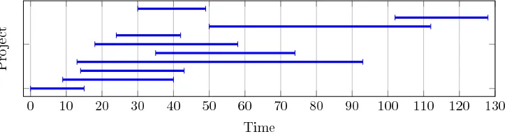
(a) Only makespan is minimised (the TPD objective is disabled), that is minimising the latest completion times of projects. TPC = 925, TMS = 119.
[image:11.595.109.472.413.509.2](b) Both objectives are enabled, that is, the primary objective is the TPD – minimising the sum of completion times of projects. TPC = 654, TMS = 128.
Figure 1: An example of overall project-level structure of good solutions (using instance B-1). Each horizontal line shows the duration allocated to each project in the schedule.
In this subsection, we report on the investigation of the natural question of what constitutes a ‘good’ approximate structure. We firstly look at the structure of a high quality schedule for a benchmark instance, and then we elucidate the observed structures using some small examples. The critical message is that optimising TPD leads to different structures of the solutions than when optimising TMS; we believe that algorithm design needs to take account of this difference.4
In particular, we have observed that in many cases, dominance by the TPD objective frequently leads to approximate ordering of the projects. A typical example of this is
4
Similar effects are also observed in [63].
given in Figure 1 using a good solution to instance B-1. Figure 1a shows the structure obtained when only the standard makespan is minimised, but the structure is very dif-ferent in Figure 1b with the required TPD-dominated objective. That is, the pattern of completion times of each project, the Cp of (3), depends on whether they are driven by
TPD, effectively minimising the average of the Cp, or instead driven by the makespan,
reducing the maximum of theCp. The example shows how, with TPD dominating, there
are time periods in the schedule when the general focus is on relatively few projects and during the schedule this focus changes between projects.
Hence, the evidence from Figure 1, and other multi-project cases we have looked at, suggests that the approximate ordering is common. Overall, these structures naturally arises from the combination of the TPD (2) objective with the limited global resources. Suppose that some P is the final finishing project, and so its last activity determines the TMS and P’ is an earlier finishing project. It may well be that P’ can move some of its activities earlier by delaying activities of P, though without changing the last activity of P. Such moves will improve the TPD without worsening the TMS.
That is, in contrast to the makespan objective, the TPD objective, together with limited shared resources, has a natural side-effect of encouraging unfairness between the finish times of projects, and will drive some projects to finish as early as possible.
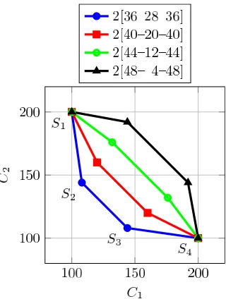
To illustrate the way in which an approximate ordering might arise, and TPD-driven and TMS-driven solutions can be quite different, we give a set of small example instances. We denote these example instances by “2[x–y–x]”, consisting of two projects. Each project consists of a precedence-constrained chain of just 3 activities of durations x, y and x, respectively. There are two (renewable) shared resources with activities 1 and 3 using the resource 2, and activity 2 using resource 1. We focus on values ofxandythat lead to resource 2 being the bottleneck, and so the main driving force of the makespan – corresponding to the shared global resource in the MISTA benchmarks. Figure 2a shows four schedules of this parametrised instance, along with their corresponding values ofC1
and C2. Solutions S4 and S3 arise from simply swapping the order of the projects in
solutionsS1 andS2 respectively.
The solutionsS1 andS4 do not interleave the two projects, and so leave gaps in the
bottleneck resource 2. In contrast, solutionsS2andS3interleave the projects and so lead
to full usage of the bottleneck resource, and are hence automatically the best solutions for the TMS objective. However, S2 and S3 are not always the best solutions for the
TPD objective. Changing the solution leads to a tradeoff betweenC1andC2, and this is
illustrated, in Figure 2b for various choices ofxandy. In this figure, the values ofxand y are selected so that we always have 2x+y= 100; this makes the effect of changing the relative balance ofxandy clearer, and also means that the values can be interpreted as percentages of the project time.
Before proceeding further, we observe that we can also interpret the project comple-tion times, Cp, from the point of view of ‘multi-objective optimisation’, by regarding
each of them as separate objectives. In particular, in standard fashion, one can say that a set of values for Cp dominates another set provided that none of the Cp values are
worse (larger) and at least one is better (smaller). One can hence discuss the cases in Figure 2b as being theCp-Pareto Front, of non-dominated sets ofCp. We emphasise this
view is for obtaining insight into the space of solutions, and is not used directly within our algorithm; we did not perform multi-objective optimisation over the Cp, though
(a) Case “2[x–y–x]”. Showing four possible
so-lutions,S1, . . . ,S4, and associated project
com-pletion times C1andC2.
(b) Tradeoff between completion times of projects. We select a range of different
val-ues forxandy, but with the invariant that
2x+y= 100; so that the effect of varying
[image:13.595.322.482.180.392.2]the balance betweenxandyis made clear.
Figure 2: Simple 2-project examples to illustrate concave and convex non-dominated sets. The notation “2[x–y–x]” means two projects each consisting of a chain of 3 tasks of durations [x, y, x] with shared resources, and the tasks 1 and 3 in each chain using resource 2, and task 2 using resource 1.
taking the pair (TPD,TMS) as a bi-objective problem, and having a (TPD,TMS)-Pareto Front (this would correspond again to a different class of algorithms than we consider here, but is again worthy of future investigation). Incidentally, there are two distinct ‘multi-objective views’ on the space of solutions:
• Cp-Pareto Front, of dimensionp, formed from the pcompletion times
• (TPD,TMS)-Pareto Front, of dimension 2, and formed from the aggregates (sum and max) of theCp
However, it is important to realise that although the Cp and (TPD,TMS) views are
different, they are tightly linked. Both the TPD, arising from P
pCp, and the TMS,
from maxpCp, are monotone (non-decreasing) with respect to the Cp and so preserve
Pareto dominance. That is, if solution Cp dominates solution Cp′, then the resulting
pair (TPD,TMS) dominates (TPD’,TMS’) – though note that the converse does not
apply. Hence, the (TPD,TMS)-Front can be extracted from theCp-Front. However, this
‘projection’ loses information; theCp-Front gives more insight into the space of solutions.
Consequently, the “Cp-Pareto Front”, or set of non-dominated Cp values, can give
some insight into the effect of TPD compared to TMS on the structure of the solutions. Hence, we can regard Figure 2b as showing the effect of thex–ybalance on theCp-Pareto
Front. In particular, we see that for two of the cases, 2[44–12–44] and 2[48–4–48] the Cp-Pareto Front is concave in terms of the set of feasible Cp values (on the top right).
When the Front is concave then the two solutions minimising the TPD areS1andS4and
are at opposite ends of the Cp-Front. In contrast, the solutionsS2 and S3 minimising
the TMS are in the middle.
Generally, with a concaveCp-Pareto Front the solutions (locally) minimisingPpCp
are naturally at the ends of the Front, and furthermore solutions at the ends of the Front will be more likely to have someCp values small and others large. This matches with the
way that the observed solutions minimising TPD do indeed sequence the projects. That is, when the projects are roughly equal size, and theCp Pareto Front is concave, then it
becomes reasonable that the TPD objective prefers the end points, and so the candidate good solutions are more likely to be widely separated in the search space.
Also, notice that as the fraction of activities using the bottleneck resource 2 (that is the value of 2x) increases, then theCp-Pareto Front becomes more concave, and the
TPD-driven solutions become different from the TMS-TPD-driven ones. This is consistent with the our general experience of the properties of MISTA instances; the shared global resource tends to be a bottleneck, and consequently they show the approximate ordering as seen in Figure 1. Future work could well use such features related to the tightness of bottle-neck resources to predict these effects, and so be used to select appropriate algorithm components. We also remark that the interesting structure of the tradeoff between the completion times does suggest that future work might well use multi-objective methods, e.g. see [10], and of course could study the effect of different weights for the completion times.
The simple example above is atypical in that the two projects are identical. However, if the projects are similar in size then it is reasonable to expect that theCp-Pareto Front
may be similar in overall structure but slightly distorted. When the front is concave but still roughly symmetric with respect to swapping the Cp, then the TPD-driven solutions
are likely to still be towards the ends of the Front and so widely separated. However, because the front is not totally symmetric the ends are likely to have slightly different values of TPD. Hence, in such circumstances, it is reasonable to expect that there may be many widely separated local optima in TPD, and also that the optima correspond to different (approximate) orderings of the projects.
4.2. MCTS
interleaved intermediate states in which the TPD is worse. We included a method to sample the space of approximate project orderings, with the intent to avoid starting in a poor ordering and being trapped.
We expect that only a partial ordering is needed because we can assume that the subsequent improvement phase can make small or medium size adjustments to the overall project ordering structure. However, the improvement phase could have more difficulty, and take more iterations, if the general structure of the project ordering were not close to the structure expected in best solutions. Consequently, and for simplicity, we decided that a reasonable approximation would be to use a 3-way partition of the projects taken to correspond to ‘start’, ‘middle’ and ‘end’ parts of the overall project time. We required the numbers of projects in each part (of the partition) to be equal – or with a difference of at most one when the total number of projects is not a multiple of 3.
The problem then is how to quickly select good partition of the projects, and the method we selected is a version of Monte-Carlo Tree Search (MCTS) methods [3]. The general idea of MCTS is to search a tree of possibilities, but the evaluation of leaves is not done using a predefined heuristic, but instead by sampling the space of associated solutions. The sampling is performed using multiple invocations of a “rollout” which is designed to be fast and unbiased. It needs to be fast so that multiple samples can be taken; also rather than trying to produce “best solutions” it is usually designed to be unbiased – the (now standard) idea being that it should provide reliable branching decisions in the tree, but is not directly trying to find good solutions.
In our case, the tree search corresponds to decisions about which projects should be placed in which part of the partition. The rollout is a fast way to sample the feasible activity sequences consistent with the candidate choice for the partition of the projects. Specifically, the tree search works in two levels; firstly to select the projects to be placed in the end part and then to select the partition between the start and middle parts.
The first stage considers5 100 random choices for the partition of the projects, and
then selects between these using 120 samples or the rollout6. The rollout consists of two
main stages:
1. Randomly select a total ordering of the activities consistent with the precedences and with the candidate partitioning. Specifically, within each partition we effec-tively consider a dispatch policy that randomly selects between activities that are available to be scheduled because their preceding activities (if any) are already scheduled.
2. Randomly select modes for the activities. If the result is not feasible then this can only be because of the mode selection causing a shortfall in some non-renewable resources. Hence, it is repaired using a local search on the space of mode selections. We use moves that randomly flip one mode at a time, and an objective function that measures the degree of infeasibility by the shortfall in resources. Since the non-renewable resources are not shared between projects, this search turned out to be fast and reliable. As a measure of precaution, if the procedure fails to obtain
5
The parameters for the MCTS were the result of some mild tuning, and used in the competition submission, but of course are adjustable.
6
The number 120 was selected so that the rollouts could be evenly distributed between 2, 4, 6, 8 or 12 cores of the machine
a feasible selection of modes after a certain number of local search iterations, we restart it with a random selection of modes.
The first stage ends by making a selection of the best partitioning, using the quality of the 25th percentile of the final solution qualities (the best quartile) of the results of the rollouts. The ‘end’ part is then fixed to that of the best partition. The decision to fix the ‘end’ part also arose out of the observation that in good solutions the end projects are least interleaved. The MCTS proceeds to the second stage, and follows the same rollout procedure but this time to select the contents of the middle (and hence start) parts. This entire process usually completes within only a few seconds, and was used as the construction stage before the much longer improvement phase. We emphasise that the TPD-structure observed earlier had an important influence of the design of the neighbourhoods used in the key improvement phase – in particular, the motivation that some moves should affect the project level structure.
5. Neighbourhood Operators
In this section, we describe our neighbourhood operators, used by several components during the improvement phase. The operators (also referred to as low-level heuristics or simply moves, depending on the algorithm which makes use of them) are categorised into three groups. This categorisation is mainly based on the common nature of the strategy the operators employ while manipulating the solution. Some of the moves are similar to those used by other submissions; see [62], and [16] and [57] for few examples. To make the paper self-contained, below we provide brief descriptions of all the moves used in our algorithm.
We guarantee that all of our operators preserve feasibility of the solution. Also, all of the moves are randomised so that they could be repeatedly used in “simulated annealing”-like improvement or applied as mutation operators. All the random selections are made at uniform unless specified otherwise.
5.1. Activity-level Operators
Operators in this category involve basic operations, widely used in the literature, such as changing the mode of a single activity or swapping the positions of two activities. On top of that, we implemented a limited first improvement local search procedure for each of the basic moves.
To describe the moves in this category, we will need additional notations. Letpos(j) be the position of activity j ∈ A within a given solution. If activity j is shifted to a different position, we say that the feasible range of its new position is [ℓ(j), u(j)], where ℓ(j) andu(j) can be computed as follows:
ℓ(j1) = (
maxj∈Pred(j1)pos(j) + 1 if Pred(j1)6=∅,
1 otherwise (7)
and
ℓ(j1) = (
minj∈Succ(j1)pos(j)−1 ifSucc(j1)6=∅,
n otherwise, (8)
• Swap activities: swap two activities in the sequence. Select an activity j1 ∈ A randomly. Select another activity j2 6= j1 ∈ A randomly such that ℓ(j1) ≤
pos(j2)≤u(j1). If ℓ(j2)≤pos(j1)≤u(j2) then swapj1 and j2. Otherwise leave
the solution intact.
• Shift: shift an activity to a new location in the sequence. Shift a randomly selected
activityj∈A to a new position randomly selected frompos(j)∈[ℓ(j), u(j)].
• Change mode: change the mode of a single activity. Select an activityjrandomly
at uniform, and if|Mj|= 1 then leave the solution intact. Otherwise select a new mode m 6= Mj ∈ Mj and, if this does not lead to a violation of non-renewable
resource constraints, updateMj to m.
• FILS swap activities: apply the first improvement local search (FILS) procedure
based on the swap move. The operator has one parameter: the width W > 1 of the window to be scanned. Select an activityj1∈Arandomly. Define the window
[ℓ′, u′] for activity j
2 as follows. Ifu(j)−ℓ(j) < W, let ℓ′ =ℓ(j) and u′ =u(j).
Otherwise select ℓ′ ∈ [ℓ(j), u(j)−W + 1] and set u′ = ℓ′+W −1. Then, for everyj2 ∈ A\ {j1} such that ℓ′ ≤pos(j2) ≤u, attempt to swap j1 and j2 (see
SwapActivities). If the attempt is successful and it reduces the objective value
of the solution then accept it and stop the search. Otherwise roll back the move and proceed to the nextj2 if any.
• FILS shift: apply the first improvement local search (FILS) procedure based on
the shift move. The operator is implemented very similarly toFILS swapActivi-ties, i.e. it attempts to shift a randomly selected activity to an new position within
a window of a given size.
• FILS change mode: apply the first improvement local search (FILS) procedure
based on the change mode move (the operator has no parameters). Select an activity j ∈A randomly. Form∈Mj\ {Mj}, produce a new solution by setting Mj =m. If the resulting solution is feasible and provides an improvement over the
original solution, accept the move and stop the local search. Otherwise proceed to the nextm∈Mj\ {Mj} if any.
5.2. Ruin & Recreate Operators
The Ruin & Recreate (R&R) operators are widely used in metaheuristics as mutations or strong local search moves but, to the best of our knowledge, they are relatively new to serial generation in scheduling. As the name suggests, such operators have two phases: the “ruin” phase removes some elements of the solution and the “create” phase reshuffles those elements (for example, randomly) and then inserts them back. The number of elements to remove and re-insert is a parameter of a R&R operator, which controls its strength (i.e. the average distance between the original and the resulting solutions).
We implemented three different types of R&R operators, and several strategies to select activities involved in the move. One can arbitrary combine any type of the R&R operator with any activity selection strategy.
The move types are Reshuffle Positions, Reshuffle modes and Reshuffle positions and modes. Reshuffle positionsmove removes all the selected activities
A′⊂Afrom the solution (leaving|A′|gaps in the sequence) and then re-inserts them in a random order while respecting the precedence relations. To determine a feasible order, we compute which activitiesVi can be placed in each gapi= 1,2, . . . ,|A′|(in terms of precedence relations between the activities inA′and activities inA\A′), and also produce a precedence relations sub-graph induced byA′. Then we apply a backtracking algorithm. In each iteration, it fills one gap, starting from the earliest gaps in the sequence. For gap i it randomly selects an activityj∈A′ such that there are no incoming arcs toj in the precedence sub-graph. If such an activity exists, the algorithm removes j from A′ and from the precedence sub-graph. Otherwise it rolls back to attempt another activity on the previous level of search. The depth of roll backs is unlimited, i.e., in the worst case, the algorithm will performs the depth first search of the whole search tree (observe that there is always at least one feasible arrangement of the activities).
Reshuffle modesmove changes the modes of selected activities while keeping their
positions intact. Each of the selected activities j ∈ A′ is assigned a randomly chosen mode, either equal or not to the previous modeMj. Observe that the new mode selection
may cause infeasibility in terms of non-renewable resources. Thus, we use the multi-start metaheuristic, simply repeating the above step until a feasible mode selection is found.
Reshuffle positions and modescombines the above two moves, which is trivial
to implement as modes feasibility is entirely independent of the sequence feasibility. We implemented several activity selection strategies some of which exploit our knowl-edge of the problem structure.
• Uniform: as the name suggests, A′ ⊂ A is selected randomly at uniform. The number of elements inA′ is a parameter of the move.
• Project: the activitiesA′ are selected within a single project, i.e.A′ ⊂A
p. The
projectp∈P is selected randomly.
• Local: the selection of activities is biased to those scheduled near a certain time
slot in the direct representation D. We randomly sample the activities accepting an activityj with probability
probability(j) = |T 1
j−τ|
width + 1
, (9)
where 0 ≤τ ≤fm(D) (see (5)) is the randomly selected time slot (the centre of
the distribution) andwidth is a parameter defining the spread of the distribution. The sampling stops when A′ reaches the prescribed cardinality.
• Global resource driven: the selection of activities is biased to the ones
sched-uled to time slots that under-utilise the global resources. The rationale is that global resources usually present a bottleneck in minimising the project completion times, and inefficiencies in the global resources consumption should be addressed when polishing the solution. In this selection strategy, as in Local selection,
we use random sampling, but the acceptance probability for an activity j ∈A is defined by
probability(j) =
P
k∈Gρremainingk(Tj)
P
k∈GρG
ρ k
where remainingk(t) is the remaining (unutilised) capacity of global resourcek at the time slott.
• Ending biased: the selection of activities is biased to the last activities within
the projects. The rationale is that, in an unpolished solution, the completion of a project might be improved by careful packing the last activities such that all the last activities end at roughly the same time, effectively maximising the utilisation of the local resources and redistributing the global resources between projects. As inLocal selectionandGlobal resource driven selection, we use random
sampling of activities. The probability of accepting an activityj∈Ais
probability(j) = project-pos(j) |Ap|
, (11)
where pis the project of activityj and project-pos(j) is the position of activityj among the activities of projectp.
5.3. Project-level Operators
It was shown in Section 4 that the TPD objective function tends to create a partial ordering of projects in high-quality solutions. The danger, however, is that the ordering to which the solution converges might be sub-optimal. Consider two well-polished solutions S1 andS2 having different project orderings. The distance between S1 and S2 is likely
to be significant with respect to the activity-level and R&R operators as many activities need to be moved to convert S1 into S2. Moreover, the transitional solutions in such a
conversion will have significantly poorer quality compared to that of S1 and S2. This
indicates that, once the algorithm converges to a certain project ordering, it needs a lot of effort to leave the corresponding local minimum and change the project ordering.
The project-level operators are designed to overcome such barriers, allowing faster exploration of the rough landscape of the MRCMPSP. They perform on the project level and thus one move of any of operators from this category usually results into a change in the project ordering. That being said, the project-level moves are likely to corrupt the solution causing many activity-level inefficiencies that need to be treated with activity-level and R&R moves. Thus, they ought to be used rarely within local search, but they can serve well as mutation operators.
In some of the project-level moves we use the formal concept of project orderingP(S). To extractP(S) from a solutionS, we compute the “centre of mass”centre(p) for each project p∈P as
centre(p) = 1 |Ap|
X
j∈Ap
pos(j)
and define the ordered set P(S) of projects according to their centres of mass.
• Swap two projects: swap two randomly selected projects in the sequence. Select
two projectsp16=p2∈P randomly. Remove all the activities belonging to projects
p1 and p2 from the sequence. Fill the gaps with all the p2 activities and then
all the p1 activities preserving the original order within each of the projects. If,
in the original solution, p1 was located earlier than p2 then the move swaps the
it simply separates them more clearly (for instance, (2,2,2,1,2,1,1,1) turns into (2,2,2,2,1,1,1,1)).
• Swap neighbour projects: swap two projects adjacent in the project ordering.
Extract the project orderingP(S), randomly select 1≤i < q and setp1 =P(S)i
andp2=P(S)i+1. Then apply theSwap two projectsmove.
• Compress project: place all the activities of a project adjacently to a new
loca-tionxin the sequence while preserving their original ordering. Randomly select a projectp∈P and remove all the activitiesj ∈Ppfrom the sequence, squeezing the
gaps (the resulting sequence will containn− |Pp|activities). Insert all the activities
j ∈Pp consecutively at position⌈x(n− |Pp|)⌉, where the parameter 0 ≤x≤1 is
the new relative location ofPp.
• Shift project: shift all the activities of a project by some offset. Randomly select
a projectp∈P and calculateposmin = minj∈Ppposj and posmax = maxj∈Ppposj.
Randomly select an offset −posmin< δn−posmax and shift every activityj ∈Pp
byδpositions toward the end of the sequence.
• Flush projects: flush the activities of one or several projects to the beginning or
ending of the sequence. Compute the project orderingP(S) and selectxconsecutive projectsP′ from P(S), where 1≤x <|P|is a parameter. Flush all the activities in projectsP to either the beginning or the ending of the sequence (defined by an additional parameter of the move).
6. Improvement Phase
Most of the time our algorithm spends on improving the initial solutions. We use a multi-threaded implementation of a simple memetic algorithm with a powerful local search procedure based on a hyper-heuristic which controls moves discussed in the pre-vious section.
6.1. Memetic Algorithm
A genetic algorithm is a population based metaheuristic combining principles of nat-ural evolution and genetics for problem solving [54]. A pool of candidate solutions (indi-viduals) for a given problem is evolved to obtain a high quality solution at the end. A fitness function is used to measure the quality of each solution. Mate/parent selection, recombination, mutation and replacement are the main operators of an evolutionary al-gorithm. However, the usefulness of recombination is still under debate in the research community [13, 38]. A recent study showed that recombination can be useful at a certain stage during the search process, if the mutations do not change the quality of resultant individuals leading to a population containing different individuals with the same fitness [56]. The choice of the recombination operator can influence the best setting for the rate of mutation depending on the problem dealt with. Although the study is rigorous, it is still limited considering that some benchmark functions, such as OneMax are used
interleaved mode of operation [47]. MAs have been successfully applied to many different problems ranging from generalised travelling salesman [19] to nurse rostering [44].
The improvement phase of our algorithm is controlled by a simple multi-threaded MA which manages the solution pool and effectively utilises all the cores of the CPU. Our MA is based on quantitative adaptation at a local level according to the classification in [43].
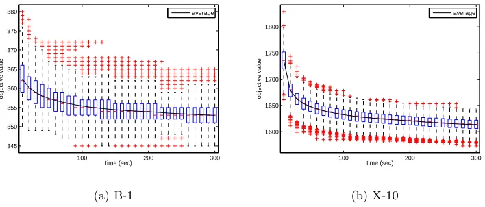
Within the MA, we use a powerful local search procedure that takes a few seconds on a single core to converge to a good local minimum. (Running the local search for a longer time still improves the solution but the pace of improvements slows down.) As the local search procedure has to be applied to every solution of the population in each generation, and the local search is by far the most intensive time consumer in our algorithm, the total running time of the algorithm can be estimated as
num-gen·pop-size·ls-time
cores ,
where num-gen is the number of generations, pop-size is the size of the population,
ls-time is the time taken by the local search procedure on one core per solution and
cores is the number of available CPU cores. Our algorithm is designed to converge within a few minutes. This implies that, to have a sufficient number of generations, the size of the population ought to be of the same order as the number of cores. On the other hand, as the memetic algorithm requires a barrier synchronisation at each generation, and our local search procedure cannot utilise any more than one CPU core, the size of the population has to be pop-size = cores·i to fully utilise all the cores, where i is a positive integer. In our implementation, we fixed the running time of the local search procedure to five seconds, and the size of the population to the number of CPU cores available to the algorithm.
Because of the small population size and limited number of generations, we decided to use a simple version of the MA, see Algorithm 6. We denote the population as S ={S1, S2, . . . , Scores}, and the subroutines used in the algorithm are as follows:
• Construct() returns a new random solution with the initial partial project sequence obtained during the construction phase (see Section 4).
• Accept(Si) returns true if the solution Si is considered ‘promising’ andfalse
oth-erwise. The function returns false in two cases: (1) f(Si) >1.05f(Si′) for some
i′∈ {1,2, . . . ,|S|}or (2) the solution was created at least three generations ago and Siis among the worst three solutions. Ranking of solutions is performed according
tofd(Si) +idle, whereidle is the number of consecutive generations that did not
improve the solutionSi.
• Select(S) returns a solution from the population chosen with the tournament selec-tion based on two randomly picked individuals.
• Mutate(X) returns a new solution produced from solution X by applying a mu-tation operator. The mumu-tation operator to be applied is selected randomly and uniformly among the available options:
– Apply theReshuffle positions and modesmove with theLocalselection
the procedure 20 times, each time randomly selecting the centre of distribution 1≤τ≤fm(D), see (9). Thewidth parameter is taken aswidth= 0.1fm(D). – Apply theSwap neighbour projectsoperator once (see Section 5.3).
– Apply the Flush projects operator with the number of selected projects
being one and flushing to the end of the sequence (see Section 5.3).
– Apply the Flush projects operator with the number of selected projects
being two and flushing to the beginning of the sequence. It was noted that the project ordering is usually less explicit at the beginning of the sequence in good solutions, and for that reason we did not use flushing single projects to the beginning in our mutations.
– Same as the last mutation except that the number of selected projects is three.
It was noted in Section 4 that the components fd(D) and fm(D) of the objective
function f(D) (see (6)) are competing. Indeed, minimisation of the total makespan favours solutions with projects running in parallel as such solutions are more likely to achieve higher utilisation of the global resources. At the same time, minimisation of the TPD favours solutions with the activities grouped by projects. Hence, the second objective creates a pressure for the local search that pushes the solutions away from the local minima with regards to the first (main) objective. To avoid this effect, we initially disable the second objective (γ←0, see Section 2) and re-enable it only after 70% of the given time is elapsed.
The parameters of the memetic algorithm (such as the ones used in the Accept(Si)
function, or the number of solutions in the tournament in Select(S)) have been chosen using a parameter tuning procedure. It should be noted, however, that the algorithm is not very sensitive to any of those parameters, which makes it efficient on a wide range of instances, and this conclusion was supported by our empirical tests, see Section 7.
6.2. A Dominance based Hyper-heuristic Using an Adaptive Threshold Move Acceptance
There is a growing interest towards self-configuring, self-tuning, adaptive and au-tomated search methodologies. Hyper-heuristics are such high level approaches which explore the space of heuristics (i.e. move operators) rather than the solutions in problem solving [5]. There are two common types of hyper-heuristics in the scientific literature [7]: selection methodologies that choose/mix heuristics from a set of preset low-level heuristics (which can both improve or worsen the solution) and attempt to control those heuristics during the search process; andgenerationmethodologies that aim to build new heuristics from a set of preset components. The main constituents of an iterative selec-tion hyper-heuristic areheuristic selectionand move acceptancemethods. At each step, an input solution is modified using a selected heuristic from a set of low-level heuristics. Then the move acceptance method is used to decide whether to accept or reject the new solution. More on different types of hyper-heuristics, their components and application domains can be found in [5, 6, 53, 45].
Algorithm 6:Improvement Phase.
1 γ←0;
2 fori←1,2, . . . ,|S|do
3 Si←Construct(); 4 end
5 whileelapsed-time ≤given-time do 6 if elapsed-time≥0.7given-time then
7 γ←0.000001 (enable secondary objective function);
8 end
9 fori←1,2, . . . ,|S| (multi-threaded) do 10 Si←LocalSearch(Si);
11 end
12 fori←1,2, . . . ,|S|do
13 if Accept(Si) =false then 14 X ←Select(S);
15 Si←Mutate(X);
16 end
17 end
18 end
6.2.1. First stage hyper-heuristic
The first stage hyper-heuristic maintains an active pool of low-level heuristicsLLH ⊆
LLHall and a score scoreh associated with each heuristic h ∈ LLH. In each iteration,
it randomly selects a low-level heuristic from the active pool with probability of picking h ∈ LLH being proportional to scoreh (line 5). Then the selected heuristic is applied
to the current solution (line 6). Initially, each heuristic has a score of 1, hence the selection probability of a heuristic is equally likely. The first stage hyper-heuristic always maintains the best solution found so far, denoted as Sbest (lines 9–11) and keeps track
of the time since last improvement.
The move acceptance component of this hyper-heuristic (lines 7–17) is an adaptive threshold acceptance method controlled by a parameterǫaccepting all improving moves (lines 7–12) and sometimes non-improving moves (lines 14–16). If the quality of a new solutionS′ is better than (1 +ǫ)f(S
best) (line 14), even if this is a non-improving move,
S′ gets accepted becoming the current solution S. Whenever S
best can no longer be
improved forelapsed-time2(in our implementationelapsed-time2= 1 sec), the parameter
ǫ gets updated as follows:
ǫ(Sbest) =
⌈log(f(Sbest))⌉+rand
f(Sbest)
(12)
where 1≤rand ≤ ⌈log(x)⌉is selected randomly at uniform. Note that 0 is a lower bound forf(S) (see Section 2) and, hence, the algorithm will terminate iff(Sbest) = 0.
6.2.2. Second stage hyper-heuristic
The second stage hyper-heuristic dynamically starts operating (lines 22–25 of Algo-rithm 7) whenever there is no improvement inf(Sbest) forelapsed-time3 (in our
Algorithm 7:LocalSearch(Si)
1 LetLLHall={LLH1,LLH2, . . . ,LLHM}represent set of all low level heuristics with each heuristic being associated with a score, initially set to 1;
2 LetSbestrepresent the best schedule;
3 S←Si;Sbest←Si;LLH ←LLHall;ǫ←ǫ(Sbest); 4 repeat
5 h←SelectLowLevelHeuristic(LLH); 6 S′←h(S);
7 if f(S′)< f(S)then
8 S←S′;
9 if f(S′)< f(Sbest)then
10 Sbest←S′;
11 end
12 end
13 else
14 if f(S′)<(1 +ǫ)f(Sbest)then
15 S←S′;
16 end
17 end
18 if NoImprovement(elapsed-time
2)then
19 S←Sbest; 20 ǫ←ǫ(Sbest);
21 end
22 if NoImprovement(elapsed-time3)then 23 ǫ←ǫ(Sbest);
24 (S,LLH)←SecondStage(Sbest,LLHall,elapsed-time
1);
25 end
26 untiltimeLimitExceeded(elapsed-time
1);
mentation elapsed-time3 = 3 sec) in line 22. The hyper-heuristic in this stage updates
the active pool LLH of heuristics. LLH ⊆ LLHall is formed based on the idea of a
dominance-based heuristic selection as introduced in [46] reflecting the trade-off between the objective value achieved by each low-level heuristic and number of steps involved. The method considers that a low-level heuristic producing a solution with a small im-provement in a small number of steps has a similar performance to a low level heuristic generating a large improvement in large number of steps. This hyper-heuristic not only attempts to reduce the set of level heuristics but also assigns a score for each low-level heuristic in the reduced set, dynamically. Those scores are used as a basis for the heuristic selection probability of each low level heuristic to be used in the first stage hyper-heuristic.
In the second stage hyper-heuristic, firstly, ǫ is updated in the same manner as in the first stage hyper-heuristic and never gets changed during this phase. Then a greedy strategy is employed using all heuristics in LLHall for a certain number of steps. Each
move in this stage is accepted using the same adaptive threshold acceptance method as described in Section 6.2.1. LLHallis partitioned into three subsetsLLHsmall,LLHmedium,
LLHlargeconsidering the number of activities processed (e.g., number of swaps) by a given
heuristic.
Small: Swap activities,ShiftandChange mode.
Medium:
• Reshuffle modes and Reshuffle positions and modes with the Uniform
selection strategy;
• Reshuffle modes and Reshuffle positions and modes with theLocal
se-lection strategy;
• Reshuffle positions and modeswith theGlobal resource drivenselection
strategy;
• Reshuffle positions and modeswith theEnd biasedselection strategy;
• Reshuffle positions and modeswith theProjectselection strategy;
• FILS swap activities,FILS shiftandFILS change mode;
Large:
• Flush projectsapplied to one project; the direction is picked randomly;
• Swap two projects;
• Compress project;
• Shift project.
At each step, each low-level heuristic is applied to the same input solution for a fixed number of iterations (5n/q for small, n/q for medium and 1 for large heuristics).7 If
7
Similar to the memetic algorithm parameters, this partition ofLLHall and the associated numbers