Analytic solutions of the Rolie Poly model in time dependent shear

Analytic solutions of the Rolie Poly model in time-dependent

shear.

George A. J. Holroyd, Samuel J. Martin and Richard S. Graham

School of Mathematical Sciences, University of Nottingham, Nottingham NG7 2RD, UK.

June 9, 2017

Abstract

We consider shear flows that comprise of step changes in the shear rate. For these flows, we derive analytic solutions of the Rolie-Poly constitutive equation. Our method involves piecing together solutions for constant rate shear in a variety of flow rate regimes. We obtain solutions for interrupted shear, recoverable strain and non-linear relaxation following cessation of flow. Whenever strong flow is present we neglect reptation, as other mechanisms dominate and for interrupted shear our solution is approximate as we neglect convective constraint release. Our analytic solutions provide new insight in several ways. These include revealing the mechanism of some experimental features of these flows; suggesting a method to extract the polymer contribution to the normal stress in the velocity gradient direction (σyy) from shear stress measurements alone; and a method to isolate the

influence of convective constraint release (CCR) from damping function measurements. We also run complementary GLaMM model calculations to verify that insight from our analytic approach translates to this more detailed model.

1

Introduction

Since the late 1970s, the Doi-Edwards Tube theory has been the key idea in the modelling of entangled polymer fluids, due to its simplicity, its parameter free prediction of the damping function, and its development into an accessible constitutive equation for the stress tensor [1]. It is built on the premise of reducing a many body problem to that of a single body in an effective mean field; encapsulating the constraints imposed upon an individual chain in a melt by its surrounding chains through the imposition of a hypothetical tube spanning the contour of the chain. Lateral movement is inhibited within the tube but the test chain is free to move diffusively along its contour; chain ends that have escaped the tube are free to explore any configuration. Both the motion of the tube and the chain within it are modelled as a random walk, with Z steps (or segments) at equilibrium [2]. The ensuing incarnations of the Tube Model are complex constitutive equations but are all still built on the simple basic idea of two types of relaxation acting on the chain in the tube: a) relaxation of polymer stretch, occurring along the contour with a timescale of the chain Rouse timeτRand b) relaxation of the polymer orientation, which

occurs at a much slower timescale of the reptation time τd ≈ 3ZτR [2]. In recent years a wide range

Molecular Dynamics, Brownian Dynamics, slip-link simulations, full chain constitutive models (such as the GLaMM model) and simpler single mode constitutive models [1]. Slip-link approaches are distinct from tube models as they make different assumptions about the confining effect of surrounding chains. A benchmark problem in this field is the description of start-up non-linear flow, at a constant deformation rate, for monodisperse entangled linear polymers.

In this paper we turn our attention to the Rolie-Poly Model, a single mode constitutive equation that was derived from more comprehensive full chain model [3]. The original intended use for this model was for computationally demanding calculations such as complex flow geometries. Indeed the model’s computational simplicity has been exploited in numerical studies of polymer processing [4–9], flow instabilities [10, 11], and shear banding [12–16]. However, the relative simplicity of the Rolie-Poly model also makes it amenable to analytic calculation. Analytic results are, in most cases, more useful than numerical results. Analytics often make analysis and interpretation more direct, more general and computationally cheaper. They are particularly useful when model parameters can be left as arbitrary constants, so that their effect can be explored directly from the analytic solution. Analytic solutions of the Rolie-Poly model have not been widely explored and are the focus of this paper. In this work we demonstrate a range of flow regimes in which the Rolie Poly Model can be solved analytically and then combine these solutions to describe the stress response to some non-standard flow histories, in which the shear rate varies with time. Such time-dependent shear flows, including interrupted shear, recoverable shear and relaxation following a step strain, have recently been explored for monodisperse entangled linear polymers [17]. Through careful analytic calculations with the Rolie-Poly model, we manage to shed greater light on the stress response in these flow experiments than has been achieved with numerical calculations alone. We then use these analytic Rolie-Poly results to guide more detailed GLaMM model calculations, to confirm that the understanding unearthed by our analytic approach translates to this more detailed model.

2

The Rolie-Poly model

We use a standard implementation of the tube model, in the form of a constitutive equation known as the Rolie-Poly model [18]. This is a single mode approximation to the tube model, which includes the three key relaxation mechanisms of reptation, retraction and convective constraint release (CCR). The Rolie-Poly model is given by,

dσσσ

dt =κκκ.σσσ+σσσ.κκκ

T₋ 1

τd

(σσσ−I)−2(1−

p

3/Trσσσ)

τR

σσσ+β

Trσσσ

3

δ

(σσσ−I)

!

, (1)

whereσσσis the polymer stress (in units of the plateau modulus),κκκis the velocity gradient tensor,β sets the CCR strength,δcontrols the suppression of CCR with chain stretch andp

Trσσσ/3 corresponds to the chain stretch ratio. The two key relaxation times are the chain Rouse timeτR, which relaxes chain stretch

and the reptation time τd. The ratio these relaxation times obeys τd/τR ≈3Z, whereZ is the number

of entanglements. Contour length fluctuations mean that higher order corrections to τd are important

model, where retraction is assumed to be instantaneous, is given by,

dσσσ

dt =κκκ.σσσ+σσσ.κκκ

T₋ 1

τd

(σσσ−I)−2

3Tr(κκκ.σσσ)(σσσ+β(σσσ−I)). (2)

For both versions of the Rolie-Poly model, start-up calculations from quiescent conditions are begun with the stress in the equilibrium state (σσσ0_=I).

We also compare our analytic results from the Rolie-Poly model with numerical solutions of the GLaMM (Graham, Likhtman and Milner, McLeish) model [3] which is a detailed implementation of all of the standard relaxation mechanisms in the tube model. The GLaMM model retains deformation information along the chain contour and so provides the most detailed stress predictions, in addition to enabling predictions of neutron scattering patterns. This model has been shown to give quantitative non-linear predictions for the shear stress and first normal stress difference of entangled linear polymers for ˙γτR . 15 [3–5]. The GLaMM and Role-Poly models, however, both predict a zero second normal

stress difference. In our GLaMM model results the stress is reported in units of the plateau modulus and times are reported in terms of eitherτe, the Rouse time of an entanglement segment, orτR=Z2τe, the

overall chain Rouse time.

3

Flows with time-dependent shear rate

Although start-up of constant rate shear is a widely used benchmark flow, flows where the shear rate changes abruptly with time have also been studied experimentally. In this section we summarise prior work on three such time-dependent protocols, which are the focus of our analytic work later in the paper.

3.1

Interrupted shear

This shear protocol involves an initial start-up shear of a quiescent melt, followed by a shear-free waiting period and then a second shear period, potentially at a different rate. By varying the rate and strain of the first shear period and the waiting time, one can explore the effect of non-quiescent initial conditions on the transient of the second shear period. For this flow protocol we denote the shear rate, time and strain for the first shear period as ˙γ1,t1 andγ1, respectively (and similarly for the second shear period)

and we denote the waiting time as tw. Wanget al. [17] performed interrupted shear experiments on an

entangled melt. Both shear rates were fast with respect to the reptation time ˙γτd >1, with ˙γ2 being

twice ˙γ1. Wanget al. [17] showed that the peak shear stress during the second shear (denotedσxymax) first

decreased withtw before beginning to increase withtw. The experiments showed a∼2.3% drop of σxymax

when comparing the lowest value with the value fromtw= 0. Standard tube models can predict this

non-monotonic behaviour, as shown by numerical solutions of the stretching Rolie-Poly model Grahamet al.

model to confirm the non-stretching result of Ianniruberto and Marrucci [22], determine shear conditions that maximise the dip and to explain the mechanism of the non-monotonic behaviour.

3.2

Recoverable shear

Recoverable strain experiments have been conducted by rheologists for many years now. For example reference [23] measured the recoverable shear strain of an LDPE melt. We focus on experiments by

Wanget al. [17] in which a start up shear of a monodisperse fluid was performed for a variety of strains

and waiting times tw, before the recoverable strain, γr, was measured. When ˙γτR < 1 or tw > τR

full chain retraction is expected to occur before the recovery, nevertheless the measured the recoverable strain was almost identical to the imposed strain (thus complete elastic recovery occurred). Wang et al. [17] claimed that retraction should substantially reduce the recoverable strain and hence that the absence of this reduction is evidence that retraction does not occur. Instead they proposed a barrier to this retraction in the Tube Model. In contrast, by computing γr from the Rolie-Poly model, Graham

et al. [20] showed that Wang et. al’s experimental recoverable strain results could be predicted without

requiring a barrier to chain retraction. Using a toy analytic calculation they proposed a qualitative reason for this lack of effect on elastic recovery. In section 4.2 we extend this result before offering a new way to utilise recoverable strain measurements to learn about the normal stress response.

3.3

Damping function

It is well established experimentally that many polymer melts obey time-strain separability following a step shear of sizeγ. That is, the non-linear shear relaxation modulus,G(t, γ) can be factorised as follows,

G(t, γ) =h(γ)G(t), (3)

where, G(t) is the linear relaxation modulus andh(γ) is thedamping function [24]. Thus the damping function is a measure of the shear thinning in response to a step strain.

4

Analytic modelling results

In the following section we employ analytic techniques and obtain closed form solutions to the Rolie-Poly model for the shear protocols described in section 3. These analytic results lead to greater insight into the dynamics of the melt in these shear regimes than numerical results alone. We solve the Rolie Poly Model for affine shear ( ˙γτR 1), a fast non-stretching shear (_τ1_d <γ <˙ _τ1_R) and stress relaxation following

shear cessation fort > τR. Building on these solutions, we derive some useful results that give us greater

insight into the experimental data discussed previously. In this section we useσσσ0 to denote an arbitrary initial stress configuration, imposed by prior parts of the flow protocol.

4.1

Interrupted Shear

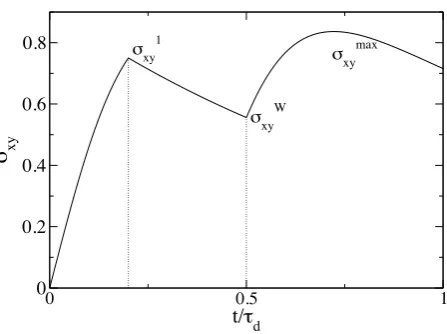
A typical stress transient for interrupted shear is shown in figure 1. For calculations herein, we denote the stress tensor at the end of the first shear asσσσ(t1) =σσσ1and the value at the end of the waiting period

asσσσ(t1+tw) =σσσW. The peak shear stress in the second shear is denotedσmaxxy and we aim to find an

analytic expression for how this depends on the shear history (ie ˙γ1,t1,twand ˙γ2).

4.1.1 Analytic calculation

0 0.5 1

t/τ_d

0 0.2 0.4 0.6 0.8

σ xy

σ_xy1

σ_xyW

σ_xymax

Figure 1: An interrupted shear flow, modelled using the non-stretching Rolie Poly Model, with ˙γ1τd =

˙

γ2τd = 5, ˙γ1t1 = 1 and tw = 0.3τd. As the flow rates are large compared to 1/τd we have neglected

the reptation term during the two flow periods, but reptation is included during the waiting period. We have also neglected CCR for these analytic calculations. We are interested in the transient shear stress maximum in the second shear period, which we callσmax

xy .

We model the shear periods using the non-stretching Rolie-Poly, neglecting reptation and CCR. Ne-glecting reptation is justified when ˙γ 1

τd and the neglect of CCR is qualitatively wrong in steady state,

but is less serious through the transient overshoot which is the focus for interrupted shear. Removing these assumptions creates small corrections but does not change the overall interpretation.

strain as the independent variable, meaning that our results depend only on strain, not independently on the shear rate and shear time, ˙γ1 andt1. That is,

dσxy

dγ =σyy−

2 3σ

2 xy,

dσyy

dγ =−

2

3σxyσyy. (4)

This nonlinear system corresponds to the rotation under shear of a rigid, slender, non-Brownian rod. Hence it can be solved via the transformation R(γ) = σxy

σyy, which gives

dR

dγ = 1. Solving for R and

substituting into equation (4) gives a separable differential equation for σyy, which can be solved and

combined with the solution forR(γ) to give,

σxy(γ) =

3(σ0

xy+σyy0 γ)

3 + 2σ0

xyγ+σyy0 γ2

, σyy(γ) =

3σ0 yy

3 + 2σ0

xyγ+σyy0 γ2

. (5)

The expression forσxy can be maximised overγ to give,

σmax_xy = 3σ

0 yy

2q3σ0

yy−(σxy0 )2

. (6)

This maximum only occurs at a positive strain ifσ0xy< q

3σ0

yy−(σ0xy)2.

We obtain a solution for the first shear period by substituting quiescent initial conditions (σσσ0 =I), into equation (5),

σ_xy1 = 3γ1 3 +γ2

1

, σ1_yy = 3 3 +γ2

1

. (7)

During the waiting time the material is allowed to relax at a fixed strain for a time tw. In this case,

relaxation of unstretched chains proceeds exponentially towardsσσσ=I, which can be seen by considering equation (2) withκκκ= 0. Hence the stress state at the end of the waiting period is,

σW_xy(γ1, tw) =

3γ1e−tw

3 +γ2 1

, σ_yyW(γ1, tw) =

3 +γ2

1(1−e−tw)

3 +γ2 1

. (8)

These stress values provide the initial conditions for the second shear period. Hence,σ_xymaxin the second shear is obtained by substituting equation (8) into equation (6),

σ_xymax(γ1, tw) =

√

3 2

"

etw_{(3 +γ}2

1)−γ 2 1 p

etw(3 +γ2

1)(etw(3 +γ12)−γ12)−3γ12 #

. (9)

This maximum must occur at a positive strain and, using the condition below equation (6), this requires,

σ_xyW >

s

3σW yy

2 ⇐⇒ 18γ2

1e−2tw

3 +γ2 1

>9 + 3γ2₁(1−e−tw_{). (10)}

If this condition is not met then the shear stress in the second shear decreases monotonically to its steady value so the maximum during the second shear is just the starting value σW

xy. We cover these two cases

with a piecewise expression,

σ_xymax(γ1, tw) =   

 

3γ1e−tw 3+γ2

1 if

σW xy<

q 3σW

yy 2 √ 3 2

etw(3+γ₁2)−γ₁2

√

etw(3+γ2

1)(etw(3+γ21)−γ21)−3γ12

ifσW xy>

q 3σW

yy

2

. (11)

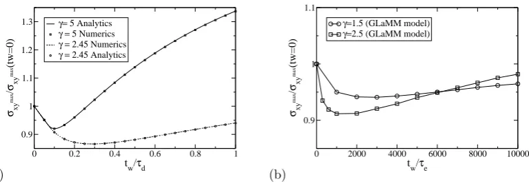
This expression is plotted in figure 2(a) and compared to direct evaluations of σ_xymax from numerical solutions of the Rolie-Poly model. Our results show a minimum of comparable size to that seen by Wang

et al. [17] experimentally, and in the classical Doi-Edwards calculations by Ianniruberto and Marrucci

(a)

0 0.2 0.4 0.6 0.8 1 t

w/τd 0.9

1 1.1 1.2 1.3

σxy

max

/

σxy

max

(tw=0)

γ= 5 Analytics

γ = 5 Numerics

γ = 2.45 Numerics

γ = 2.45 Analytics

(b)

0 2000 4000 6000 8000 10000 t

w/τe 0.9

1 1.1

σxy

max

/

σxy

max

(tw=0)

γ=1.5 (GLaMM model)

γ=2.5 (GLaMM model)

Figure 2: (a) Our piecewise Rolie-Poly solution (equation (11)), normalised byσxymax(γ,0) for each strain.

An initial strain of γ ≈ 2.45 admits a drop of ≈ 13%, which is in fact a little larger than that seen experimentally. (b) GLaMM model predictions comparing the strain used in the experiments of Wanget al. [17] (γ= 1.5) with a strain close the optimum predicted by our analytic model.

As we have an analytic expression forσmax

xy , we can readily optimise the depth of the minimum with

respect toγ1 andtw. Our numerical minimisation of

σmax_xy (tw)

σmax

xy (tw=0) from equation (11) shows that an initial

strain of ≈2.45 admits the deepest minimum of ∼13%, occurring at tw ≈ 0.25. This result suggests

that a somewhat deeper minimum might have been found in the experiments of Wang et al. [17] by extendingγ1 from 1.5 to ∼2.5. However, we note that the approximations in our calculations, namely

using the Rolie-Poly model and neglecting reptation and CCR during shear, generally produces sharper features than seen experimentally so the measured dip may be smaller than we predict. Indeed, we checked that this prediction of our analytic model is obeyed by the more detailed GLaMM model, which has been shown to give quantitative predictions for non-linear shear rheology [3]. For these GLaMM model calculations we used Z = 40, ˙γ1τR = ˙γ2τR = 0.16 and retained all processes, including contour

length fluctuations, CCR and chain stretching. Figure 2(b) shows that, as anticipated,γ1= 1.5 gives a

shallower minimum of∼6% compared toγ1= 2.5 which gives a minimum of∼9%.

4.1.2 Explanation of the mechanism

We now turn our attention to explaining the mechanism that produces the non-monotonic behaviour in

σmaxxy with increased relaxation time. We will show that relaxation and flow together allow access to a

wider region of the initial conditions for shear 2 (σxyW andσyyW ) than flow alone. Some of these regions give

a weaker σ_xymax than those that can be accessed by the shear 1 alone. From the differential equation for

σxy, equation (4), we can see that the first term on the RHS, which corresponds to convection, controls

the growth of σxy and this growth is proportional to σyy. σyy reduces as shear flow progresses and

increases during the waiting period. This recovery ofσyy during waiting period the gives stronger and

more sustained growth inσxy during the second shear, leading to a largerσmaxxy . In summary, too much

pre-alignment ofσyy leads to a weak maximum and which is improved by relaxation. Considering now

the effect of initial value ofσxy at the start of the second shear, a larger initial value, σxyW, produces a

(a)

0 0.2 0.4 0.6 0.8 1 σ_yy

0 0.2 0.4 0.6 0.8 1

σxy

No maximum during shear 2

Waiting period

Shear 1

(b)

0.5 0.6 0.7 0.8 0.9 1 σ_yy

0 0.1 0.2 0.3 0.4 0.5 0.6 0.7

σxy

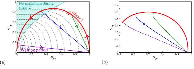
Figure 3: (a) A phase portrait of (σyy, σxy) during shear and relaxation, overlaid on a contour plot of

the maximum inσxy achieved during shear period 2 from the initial conditionsσyy,σxy. The thick lines

correspond to the evolution of (σyy,σxy) during a start-up shear from rest (curved line) and relaxation

following shear (diagonal lines). The strain during shear 1 for these diagonal lines are γ = 20,2.45,1 from left to right, respectively. The grey dashed lines are contours of the maximum in σxy achieved

during the second shear period, corresponding to σmax

xy = 0.1...0.85 in evenly spaced intervals of 0.05,

with the smaller contours occurring closer to the origin. (b) Similar results from the GLaMM model, for

γ1= 1.5,2.5 and 5.0. The stars correspond to theσyy-σxy values that leads to the lowestσxymax.

increase in the retraction term, which is proportional to -σ2

xy, giving a comparatively weak dependence

of the maximum onσxy at larger values. In summary, the decrease inσxy during relaxation reduces the

maximum, but this effect is weak at largeσxy.

In the paragraph above we explain the contributions ofσW

xy andσWyy to σmaxxy . We now explain how

shear and relaxation work together to produce a smaller σmax

xy . In fig 3(a) the solid lines represent the

evolution ofσxy andσyy during shear 1 (circular red line) and the waiting period (diagonal lines, other

colours). The analytic solutions in equations (4) and the exponential relaxation during the waiting period provide the forms of these lines in the phase-plane. The dashed lines are contours ofσxymaxobtained from

takingσyy,σxy as the initial conditions. The strain in shear 1 (red line) determines the exit point from

the flow-circle and this determines the angle in the σxy-σyy plane by which the system returns to the

quiescent state (σxy = 0,σyy = 1). This angle determines the relative rate of change of σxy compared

to σyy during relaxation. The purple line in fig 3(a) illustrates a strain that is too large to produce

non-monotonic behaviour inσmax

xy . Here the decrease inσxy during relaxation is small compared to the

increase inσyy, meaning that the maximum grows with increased waiting time. Note how the purple line

slices through several contours of σmax

xy but this corresponds to increasing σmaxxy as σyy is increasing at

roughly fixedσxy. Conversely, following a small strain in shear 1 (green line)σxyhas the further of the two

stresses to relax and so changes faster than σyy, giving a reduction in the achieved maximum. However,

this reduction is modest as σxy1 itself is small. The deepest maximum occurs at a point intermediate to

these two exemplars (blue line), which is just beyond the quiescent transient maximum inσxy. The angle

of this relaxation period cuts through the optimum number ofσmax

xy contours in the decreasing direction.

only a very limited range of initial conditions for the second shear period. The waiting period corresponds to exponential relaxation, which, when combined with different choices of the strain allow access to a far wider region of the σxy-σyy plane as initial conditions for shear 2. Some the regions of this space

that are only accessible by relaxation give a weaker shear 2 maximum than those that can be accessed by the first shear period alone. We confirm that the mechanism is the same in the GLaMM model by plotting our results as a phase-portrait in figure 3(b). This shows very similar behaviour to figure 3(a), namely that the shear causes an arc inσxy-σyy,γ1determines the point of exit from this arc, the waiting

period causes a linear return to the quiescent state and that the point in the σxy-σyy plane that gives

the lowestσmax

xy occurs in very similar places for both models. There are two minor differences: the arc

is incomplete for the GLaMM model because CCR leads to non-zero steady state values forσxy andσyy;

and the initial behaviour ofσxy-σyy during the waiting period is not linear due to some fast processes

that are neglected in our analytic calculations (retraction, CCR and contour length fluctuations). We have solved analytically the non-stretching Rolie-Poly model in the absence of CCR and reptation, for the entire interrupted shear transient. We also derived an analytic expression for the second shear maximum. We used this analytic expression in a numerical optimisation to find the shear conditions that lead to the deepest reduction inσmax

2 . Our analytic result also explains the mechanism of the

non-monotonic behaviour seen the GLaMM model, suggesting that this mechanism explains the experiments of Wang et al. [17].

4.2

Recoverable strain

In this section we propose an analytic approach for recoverable strain in well-entangled polymers. During a recovery flow the shear rate varies with time according to a balance between the polymer stress and the Newtonian viscosity from the fast modes of the melt. We model this by a rapid reversing shear flow, which is valid for the following reasons: the ratio of the polymer zero shear viscosity and the Newtonian viscosity is very large for entangled melts [13, 27], meaning that, the majority of the strain recovery occurs at very high shear rates. For these high shear rates the time-dependence of the shear rate is unimportant and the polymer configurations depend only on the total strain. This has been confirmed numerically for the Rolie-Poly model [20]. Thus we model recoverable strain by a rapid, reversing shear and define the recoverable strain as the strain at whichσxy passes through zero.

Care must be exercised over the generality of this correspondence between recoverable strain and rapid reversing flow. It relies upon separating all relaxation processes as either strongly non-linear ( ˙γτ 1) or Newtonian ( ˙γτ 1). Any process for which ˙γτ ∼1 must make a negligible contribution to the total stress. This is equivalent to a strong separation of relaxation times in the materials relaxation spectrum. This is demonstrably true for well-entangled linear polymers, as can be seen by the long elastic plateau in

G0_{(ω). However, if the linear relaxation spectrum contains important relaxation modes for all timescales}

shorter than the terminal time, as will be the case for weakly entangled polymers, polydisperse polymers and many other rheological fluids, then the correspondence does not hold.

Modelling recoverable strain as a fast (affine) reversing flow, means we retain only the convection terms in the constitutive model, which becomes (see Appendix A.1),

dσxy

dt =−γ˙(t)σ

0 yy =⇒

dσxy

dγ =−σ

0

That is, the gradient of the shear stress with reversing strain is simply σ0

yy, namely the value of σyy at

the end of the first shear period. We note here thatσσσdenotes the polymer contribution to the stress, not the total stress. Since the recoverable strainγr, is the strain at whichσxy passes through 0 we obtain,

γr=

σ0 xy

σ0 yy

. (13)

4.2.1 The effect of retraction

In this section we show that chain retraction has no direct effect on the recoverable strain. The contri-bution to the stress relaxation from retraction is given by,

dσσσ

dt =....−

21−q 3 trσσσ

τR

σσσ. (14)

We note that this can be written as,

dσσσ

dt =...−f(Trσσσ)σσσ, (15)

where the form of the function f(Trσσσ) will be unimportant to the argument in this section. From equation (15) we see that retraction scales all components ofσσσdown at an equal rate, so under its effect alone the ratio γr =σxy/σyy is unchanged. More explicitly, we can obtain the same result by directly

differentiating the this ratio and (and using equation 15),

dγr

dt =...+

σyyσ˙xy(t)−σ˙yy(t)σxy

σ2 yy

=....+ 0. (16)

Thus we can see from the above argument that retraction, either during or after flow, does not directly affect the recoverable strain and that this result is insensitive to the form of the retraction function. In appendix A.2.1 we use a similar argument, involving the mathematical structure of the retraction term, to show that the damping function is also independent of the form off(Trσσσ).

An alternative way of interpreting this result was recently proposed by Larson [28], which is as follows. The recoverable strain corresponds to the reversing strain required to return the shear stress to zero. This strain is set entirely by the orientation, and stretching or compressing the chains at fixed orientation has no effect on the strain required to reset the shear stress. Hence chain retraction has no effect on the recoverable strain.

4.2.2 Application to experiments and simulations

0 1000 2000 3000 4000

t/τ_e

0 0.5 1 1.5

σ

σxy(direct calculation) σ_yy(direct calculation)

σyy(from reversing flow)

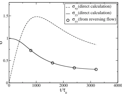
Figure 4: Results for the GLaMM model, comparing the direct transient calculation of σyy with values

inferred from a rapid reversing shear.

We note that our results above offer an in-principle method to access experimentally the polymer contribution to the normal stress componentσyy from measurements made only on the shear stress (via

a simple rearrangement of equation (13)). This is attractive as normal stresses are significantly more difficult to measure than shear stress. To test that the result holds when we resolve faster processes in tube model, such as contour length fluctuations and higher retraction modes, we applied the technique to the GLaMM model. We ran a start-up shear calculation with Z = 40 and ˙γτR = 4.8, to produce

the transient stress curve shown in figure 4. At selected points along the transient we began a rapid reversing shear and obtained the recoverable strain from the strain required to returnσxy to zero. From

this recoverable strain we estimated σyy at the start of the reversing flow via equation (13). Figure 4

shows that σyy estimated from the reversing flow agrees very well with the directly calculated value,

indicating that our result derived from the Rolie-Poly model also holds for the GLaMM model. These calculations show that, even when we include the full gamut of tube model processes, the GLaMM model still predicts thatσyy can be extracted fromσxymeasurements alone. This provides a strong imperative

for further testing via molecular dynamics and experiments. Finally, recoverable strain experiments by

Wanget al. [17], showing that retraction has no effect on the recoverable strain, are consistent with our

results on reversing flow, and hence provide indirect experimental support

To further support this proposed experimental approach, it would be useful to verify that our result holds for Molecular Dynamics (MD) simulations. MD offers a way to verify the connection between rapid reversing flow and normal stress components. We have in mind a flow geometry in which shear is applied in the usual xy direction and is then followed by a two separate rapid shear flows, the first a reversing flow in the usual shear geometry and the second in an orthogonal direction. In appendix B we show that an affine shear in theα-β direction leads to the stress response

σαβ(γ) =σαβ0 +γσ 0

ββ. (17)

Thus shearing in a new geometry with velocity gradient direction β, reveals information about the ββ

normal stress from the previous shear. Hence to accessσxxone must shear in theyxorzxdirection, which

with the first normal stress difference extracted from MD in the usual way, by considering all pairwise interactions. This comparison would provide further support for the connection betweenσyy and reversing

shear, to motivate experiments to extract σyy from shear stress measurements that are achievable in

standard rheometers.

Regarding experiments, we note that an orthogonal shear geometry has been realised in the experi-ments of references [29] and [30]. However, in these experiexperi-ments the velocity gradient direction remains in they-direction so then they are sensitive toσyy, the same as reversing shear. It is not presently clear

how such a flow geometry, with a change in velocity gradient could be realised in experiments.

4.3

Shear damping function

In this section we derive an analytic expression for the shear damping function predicted by the Rolie-Poly model for well entangled polymers.. Following a large step strain, for t _. τR the shear stress initially

drops rapidly, due to retraction. At later times t _& τd the remaining stress relaxes according to the

linear relaxation spectrum. Between these two timescales the stress remains approximately constant at a plateau value and this plateau value directly determines the damping function. We compute the plateau from the Rolie-Poly model based on the following physical ideas: chain stretch is fully relaxed at the plateau, no reptation occurs until after the plateau, the time dependence of the chain retraction does not affect the plateau, provided it fully relaxes chain stretch on a timescale ofτR.

We consider a long-chain polymer melt (Z 1, so τd and τR are well separated) and apply a fast

step strain ( ˙γ >>1/τR), with a total strain ofγ. As the flow is affine the stress tensor immediately after

the flow is given by σ0

xy =γ, Trσσσ0=γ2+ 3 andA0xy= σ0

xy

Trσσσ0 = 3γ

γ2₊₃ (see appendix A.1). Following the

flow, the material will relax via retraction and CCR to reach some plateau σ_xy∞ at t≈τR. We found an

analytic expression for this plateau in appendix A.2 by neglecting reptation and considering long-time solutions of the Rolie-Poly model. Using equation (38) with the affine initial conditions above gives,

σ_xy∞= 3γ

3 +γ2Θ(γ), (18)

where,

Θ(γ) = exp β

Z 3

γ2₊₃

(u/3)δ−1

u+β(u/3)δ_(u−3)du !

. (19)

Note that this result forσ∞

xyis independent of the time dependence of the relaxation due to retraction, in

accord with our expectation above. We only require that retraction scales down equally all components of the stress and relaxes Trσσσto reach its equilibrium value of 3 before significant reptation occurs (see appendix A.2 for mathematical details). Once the plateau is achieved the stress relaxes exponentially from a stretch-free state as detailed in section 4.1, so can be written as,

σxy(t) =σ∞xy=

3γ

3 +γ2Θ(γ)G(t), (20)

whereG(t) = exp−t τd

is the linear relaxation function.

We now compare equation (20) with the expression for time-strain separability (valid fort > τR),

G(t, γ) = σxy(t)

whereh(γ) is the damping function. Rearranging equation (21) substituting into this equation (20) leads to our expression for the damping function,

h(γ) = σ

∞

xy

γG(t) = 3

3 +γ2Θ(γ). (22)

We see that h(γ) is the product of two factors. The term 3

3+γ2 corresponds to the direct retraction

contribution, in the absence of CCR, as predicted by the differential approximation to the Doi-Edwards model [31, 32] and Θ(γ), which is the CCR correction.

4.3.1 Evaluating the CCR integral forδ=−1

2 and β = 1

To obtain a closed-form expression for the damping function we are required to perform the integral in equation (19). This is straightforward in some cases, such as δ= 0 (see appendix A.2), which leads to the following direct expression for the damping function,

h(γ) = 3

3 +γ2_{(1 +β)}. (23)

However, when δ=−1/2 and β = 1, which are the values recommended for the Rolie-poly model [18], the integral is possible but more involved. Substituting the values for δ and β into equation (19) and following the integration strategy in appendix A.2.5 leads to,

Θ(γ) = (γ

2_{+ 3)}

(D+pγ2_{+ 3)}C_(G2_{+ (F+}p

γ2_{+ 3)}2₎Eexp B−Aarctan

G

F+pγ2_{+ 3} !!

. (24)

All of the lettered quantities are constants, given in table I.

Table I: Numerical evaluation of the constants in equation (24). For details of their derivation see appendix A.2.5

A B C D E F G

-0.5524 -0.53834 0.82299 -1.30749 0.5885 1.51977 1.29014

0.1 1 10

γ 0.001 0.01 0.1 1 h( γ) Experiments β=0 β=1 Numerics (a)

0.1 1 10

γ 0.01 0.1 1 h( γ) Experiments Cv=0 (no CCR) Cv=0.1

(b)

10-2 ₁₀-1 ₁₀0 ₁₀1 ₁₀2

γ 0.5 0.6 0.7 0.8 0.9 1.0 1.1

Θ(γ) = (γ

2+3) h( γ)/3 Numerics Analytics β=0 (c)

Figure 5: Damping function plots, with and without CCR, compared to experiment data from Osaki

et al. (1982)[33] (symbol fills indicate different molecular weights). (a) Rolie Poly results for analytics

(equation (22)) and numerics (δ=−1

2,β = 1). (b) GLaMM model results. (c) Rolie Poly results for the

4.3.2 Discussion

Figure 5(a) compares our analytic approach with numerical results for the Rolie-Poly damping function, and includes experimental data. Figure 5(b) compares the GLaMM model predictions, with and without CCR, with experimental data. For both models the predictions without CCR are already somewhat lower than the experiments, and including CCR further worsens the agreement. Thus, it appears that improving the self-consistency of the tube model through CCR diminishes its predictive ability. However, primitive chain network simulations by Furuichi et al [34] have produced quantitative agreement with these damping function measurements. These simulations include all standard tube model relaxation processes, and also include a force balance around entanglements (FB), which is absent from the GLaMM and Rolie-Poly models. As the GLaMM model predicts well the start-up of constant rate shear, it seems likely that the effect of FB is particularly important to describe the very rapid step strain required for damping function measurements, but is less important for continuous flow. Thus, our analytic approach may find use in computing analytic expressions for the damping function for future models that include both CCR and FB. We note also that our analytic approach can describe stress relaxation from arbitrary initial conditions so may be useful, in its current form, to describe the non-linear relaxation following deformation from fast, but not instantaneous, strain rates.

The damping function is strongly strain dependent, dropping off nearly two decades for strains between 1 and 10, largely due to the direct retraction contribution. To expose the effect of CCR in the Rolie-Poly model, in figure 5(c) we have extracted directly the CCR contribution Θ(γ) by dividing through by

3

3+γ2. In this plot the y-axis is much more compressed, which exposes both the CCR contribution and

finite Z effects at large strain, where the analytics and numerics begin to disagree slightly. Numerical results were run with Z ≈ 300, whereas full suppression of reptation (Z = ∞) would be needed for complete agreement with the analytic results. This may develop into a useful way to extract the CCR parameters from non-linear stress relaxation experiments or molecular dynamics simulations, particularly if the influence of FB can be controlled by reducing the flow rate used to impose the initial strain.

Our analytic approach shows how the damping function is insensitive to the exact mathematical form of the retraction function. Furthermore, the damping function is also somewhat insensitive to CCR. This can be contrasted with start-up non-linear flows that are sensitive to the details of both retraction and CCR. Thus early versions of the Doi-Edwards model predicted the damping function without requiring detailed treatment of constraint release, contour length fluctuations and retraction, even though a full treatment of these processes was required for quantitative agreement for most other stress measurements. The simulations of Furuichi et al [34] also suggest that errors due to omitting CCR and FB cancel to some extent in the Doi-Edwards model.

5

Conclusions

Interrupted shear measurements by Wang et al. [17] of the second shear stress maximum (σmax

xy )

show a monotonic dependence on the waiting time. Our analytic solution illustrates that this non-monotonic behaviour occurs because relaxation and flow together allow access to a wider region of the initial conditions for shear 2 than flow alone. The non-monotonic response arises because some of these regions give a lowerσmaxxy than those accessible by the shear 1 alone. By minimising our analytic expression

forσmax_xy we could find the interrupted shear conditions that give the most strongly monotonic behaviour. Our analytic results for recoverable strain, valid for well entangled polymers, suggest that recoverable strain can be found equivalently by a rapid reversing flow. This result illustrates why chain retraction has no direct effect on the recoverable strain. Furthermore our approach suggests a method to access

σ0

yy (the polymer contribution to the yy stress at the beginning of the reversing shear) through shear

stress measurements alone. We showed that this result hold for the more detailed GLaMM model. We also proposed a further validation of this result using molecular dynamics simulations to establish a link between the normal stress and orthogonal shear. These results together would provide a strong imperative for further testing via experiments.

In deriving an analytic expression for the damping function in the Rolie-Poly model we showed that the damping function is insensitive to the time-dependence of the retraction term and only moderately sensitive to CCR. This explains how early versions of the Doi-Edwards model could capture quantitatively measurements of the damping function despite missing details that are necessary to describe other stress measurements. Our calculation suggests a new plot of data for non-linear stress relaxation following cessation of flow that isolates the CCR contribution. This plot is potentially useful as it is sensitive to details of CCR but is comparatively insensitive to other relaxation processes such as retraction, contour length-fluctuations and reptation. Results for this plot, from either experiments or molecular dynamics simulations, could be used to test and improve CCR assumptions and parameters in constitutive models. Simulation results [34] suggest that the force balance at entanglement points also needs to be considered to fully capture damping function measurements, but this may be alleviated by considering relaxation following a non-instantaneous deformation.

As the Rolie-Poly model incorporates the key non-linear mechanisms of the tube model, its results are strongly representative of the tube model, in general. To highlight this we produced for all calculations, complementary GLaMM model calculations. It is important to note that our choice of flow conditions for these more expensive calculations was specified by our analytic results. That is, from the analytic results, we knew which longer calculations to run with the more detailed model. Furthermore, the key features from our Rolie-Poly results were also seen in the GLaMM model calculations. Thus, as the GLaMM model accurately captures non-linear shear experiments, this establishes a link to rheological experiments.

Acknowledgements

The authors thank Peter Olmsted and Zuowei Wang for very useful discussions about this work. We also thank Ron Larson for very useful discussions, particularly for his explanation of our result concerning the effect of retraction on recoverable strain.

A

Analytic solutions from arbitrary initial conditions

Many of the calculations in this paper involve step changes in the shear rate, between periods of constant rate shear. We can model this piecewise constant shear history as a series of constant rate shear flows, in which the ending stress-state of the system becomes the initial condition for the next shear period. Thus throughout this appendix, we model a system that has experienced some pre-shear in the xy direction that leads to the following stress-state,

σσσ=



  

σ0

xx σxy0 0

σ0xy σ0yy 0

0 0 σ0zz 

  

, (25)

which we take as the initial condition for the next shear period, which is also in the xy direction but with a new rate. We leave the values of the components of the initial stress state as arbitrary numbers throughout. Starting with these initial conditions we then consider separately three scenarios: affine shear, relaxation following a non-stretching flow and retraction and CCR following flow. These are detailed individually below.

A.1

Affine Shear

This affine shear calculation will be useful in deriving expressions for the recoverable strain. Suppose a melt is sheared at a very high rate |γ˙| 1

τR. Then all relaxation (and so all the nonlinear terms) can

then be ignored, and the system reduces to

dσxy

dγ =σyy,

dσyy

dγ = 0, (26)

which has the solution

σxy(γ) =σxy0 +γσ0yy, σyy =σ0yy. (27)

for arbitrary initial values.

A.2

Retraction and CCR following flow

Here we consider relaxation following a large arbitrary shear flow. We consider a highly entangled material so that there is a clear plateau in the stress relaxation, occurring when retraction is complete but reptation has not yet begun (τR< t < τd). We derive an analytic expression for this stress plateau,

which can be used to calculate the damping function of the Role-Poly model.

Consider the stretching Rolie-Poly model following a shear strain in the limit ofτd → ∞, we analyse

the long-time stress plateau of this model following this strain. The overall equation is,

dσσσ

dt =−f(Trσσσ)

where f(Trσσσ) is the retraction rate. In the original Rolie-Poly modelf(Trσσσ) = 2(1−p

3/Trσσσ)/τR but

our results here will turn out to be independent off (provided f(3) = 0). The absence of flow removes much of the coupling. In particular, taking the trace of eqn (28) gives a closed equation for Trσσσ. If a solution for Trσσσ(t) can be found then, the remaining components ofσσσeach obey an independent linear ODE.

A.2.1 Trace equation

Taking the trace of eqn (28) gives a differential equation for Trσσσ,

dTrσσσ

dt =−f(Trσσσ)

h

Trσσσ+β(Trσσσ/3)δ(Trσσσ−3)i. (29)

We will see later that we do not need to solve this equation for Trσσσ(t), we just need to note that Trσσσ(t) obeys this equation.

A.2.2 Orientation equation

We suppose here that we have a solution for Trσσσ(t) from equation (29), which we denoteT(t). We now define the orientation tensor,

A= 3σσσ

Trσσσ. (30)

Following a shear strain the long-time solution of eqn (28), after all chain stretch has relaxed, will be

σσσ=A. Implicitly differentiating equation (30) gives,

dA

dt =

3 Trσσσ

dσσσ dt −

σ σ σ

Trσσσ dTrσσσ

dt

. (31)

Substituting in equations (28) and (29) and, as Trσσσ is a known function of time, T(t), we obtain a

diagonal, linearset of ODEs forA,

dA

dt =−Ψ(t)(A−I), (32)

where,

Ψ(t) =βf[T(t)]

_T(t)

3

δ−1

. (33)

A.2.3 Long-time solution

Eqn (32) can be solved by the integrating factor method. We examine here just the shear component

Axy in the limitt→ ∞(the full time-dependence and other components are readily obtained in the same

way),

A∞_xy=A0_xyexp

−

Z ∞

0

Ψ(t)dt

. (34)

HereA0

xy is the shear orientation immediately following some previous shear period.

A.2.4 Simplifying the integral

We now consider the integral

I=

Z ∞

0

Ψ(t)dt,

=

Z ∞

0

βf[T(t)]

_T(t)

3

δ−1

dt.

We can make the change of integration variable u=T(t). This givesdt= 1

T0_(t)du, with the new limits

u=T0 andu= 3, being the initial conditions and the long-time solution to equation (29). This gives,

I=β

Z 3

T0

1

T0_(t)f[u]

u

3

δ−1

du. (36)

Now using eqn (29) for T0(t) cancels out thef[u] to give,

I=−β

Z 3

T0

(u/3)δ−1

u+β(u/3)δ_(u−3)du. (37)

Thus we see that the long-time plateau is given by

A∞_xy=A0_xyexp β

Z 3

T0

(u/3)δ−1

u+β(u/3)δ_(u−3)du !

. (38)

A.2.5 Carrying out the integral

Integer δ

We note that when δ is an integer then the integrand in equation (37) is a ratio of polynomials. Thus the integrand can be separated by partial fractions into a sum of simpler rational functions that can be integrated individually. Once |δ| >2 then the order of the polynomials becomes large enough that the factorisation required for partial fractions becomes awkward to express in a convenient closed form, but nevertheless the analytic method still exists. We show here as an exemplar δ = 0. When δ = 0 the integral reduces to,

I= ln(1 +β−3β/T0). (39)

We obtain an expression for the long time value ofAxy by combining equations (34) and (39), to get the

remarkably simple result,

A∞_xy= A

0 xy

1 +β−3β/T0

. (40)

Rational δ

Ifδis a rational number then the strategy for integerδ above, can be used once a change of integration variable (such asv=u−δ) has been applied. If the either the numerator or denominator of the irreducible form ofδare much larger than one, then the integration will involve factorising a high order polynomial. Here we presentδ=−1/2 as an exemplar since this is the value recommended for the Rolie-poly model [18]. Substitutingδ=−1/2,β= 1 and v=u1/2 _{into equation (37) gives,}

I=

Z

√

T0

√

3

6.33/2

v4₊√_3v(v2₋₃₎dv. (41)

Factorising the denominator, applying partial fractions and integrating leads to

I=

"

2 lnv−2

3 X

i=1

√

3 +λi

2√3 + 3λi

ln(v−λi) #

√

T0

3

, (42)

where theλi are the roots of the following cubic equation: x3+

√

3x2₋₃√_{3, of which two are a complex}

B

Orthogonal Strain in the

α

-

β

direction

We now consider orthogonal shear flow. That is, shearing in a plane at a right angle to the usual xy

shear direction. This is motivated by our observation that reversing shear in thexyprovides information about the normal stress componentσyy and also by the orthogonal shear experiments of references [29]

and [30]. Suppose we begin with an arbitrary, symmetric stress tensor and apply an affine shear in a new plane that we call theα-β direction, whereαandβ are one of the usual Cartesian axes andα6=β. That is, we impose a velocity gradient tensorκκκsuch thatκαβ= ˙γ and all other components ofκκκare zero. We

now consider the rate of change of the shear stress in theα-β direction. For an affine flow we have,

dσαβ

dt = κκκ.σσσ+σσσ.κκκ

T

αβ= ˙γσββ, (43)

where we have substituted the form of κκκ described above. Solution of this equation takes the form (substitutingγ= ˙γt),

σαβ(γ) =σαβ0 +γσ0ββ. (44)

That is, in the new shear plane the shear stress gradient with respect to strain is the normal stress component in the velocity gradient direction.

References

[1] McLeish, T. C. B., “Tube theory of entangled polymer dynamics,” Advances in Physics51, 1379–1527 (2002).

[2] Larson, R. G. and P. S. Desai, “Modeling the rheology of polymer melts and solutions,” Annu. Rev. Fluid Mech.47, 47–65 (2015).

[3] Graham, R. S., A. E. Likhtman, T. C. B. McLeish and S. T. Milner, “Microscopic theory of linear, entangled polymer chains under rapid deformation including chain stretch and convective constraint release,” J. Rheol.47, 1171–1200 (2003).

[4] Bent, J., L. R. Hutchings, R. W. Richards, T. Gough, R. Spares, P. D. Coates, I. Grillo, O. G. Harlen, D. J. Read, R. S. Graham, A. E. Likhtman, D. J. Groves, T. M. Nicholson and T. C. B. McLeish, “Neutron-mapping polymer flow: Scattering, flow-visualisation and molecular theory,” Science 301, 1691–1695 (2003).

[5] Collis, M. W., A. K. Lele, M. R. Mackley, R. S. Graham, D. J. Groves, A. E. Likhtman, T. M. Nicholson, O. G. Harlen, T. C. B. McLeish, L. R. Hutchings, C. M. Fernyhough and R. N. Young, “Constriction flows of monodisperse linear entangled polymers: Multiscale modeling and flow visual-ization,” J. Rheol.49, 501–522 (2005).

[6] Graham, R. S., J. Bent, L. R. Hutchings, R. W. Richards, D. J. Groves, J. Embery, T. M. Nicholson, T. C. B. McLeish, A. E. Likhtman, O. G. Harlen, D. J. Read, T. Gough, R. Spares, P. D. Coates and I. Grillo, “Measuring and predicting the dynamics of linear monodisperse entangled polymers in rapid flow through an abrupt contraction. a small angle neutron scattering study,” Macromolecules

[7] Valette, R., M. R. Mackley and G. H. F. D. Castillo, “Matching time dependent pressure driven flows with a rolie poly numerical simulation,” Journal of Non-Newtonian Fluid Mechanics 136, 118–125 (2006).

[8] McLeish, T. C. B., N. Clarke, E. de Luca, L. R. Hutchings, R. S. Graham, T. Gough, I. Grillo, C. M. Fernyhough and P. Chambon, “Neutron flow-mapping: Multiscale modelling opens a new experimental window,” Soft Matter5, 4426–4432 (2009).

[9] Liu, Q., J. Ouyang, C. Jiang, X. Zhuang and W. Li, “Finite volume simulations of behavior for polystyrene in a cross-slot flow based on rolie-poly model,” Rheologica Acta55, 137–154 (2016).

[10] Hassell, D. G., M. R. Mackley, M. Sahin, H. J. Wilson, O. G. Harlen and T. C. B. McLeish, “Molecular physics of a polymer engineering instability: Experiments and computation,” Phys Rev E

77, 050801 (2008).

[11] Reis, T. and H. Wilson, “Rolie-poly fluid flowing through constrictions: Two distinct instabilities,” Journal of Non-Newtonian Fluid Mechanics195, 77–87 (2013).

[12] Adams, J. M., S. M. Fielding and P. D. Olmsted, “Transient shear banding in entangled polymers: A study using the rolie-poly model,” J Rheol55, 1007 (2011).

[13] Agimelen, O. S. and P. D. Olmsted, “Apparent fracture in polymeric fluids under step shear,” Phys Rev Lett110, 204503 (2013).

[14] Cromer, M., M. C. Villet, G. H. Fredrickson and L. G. Leal, “Shear banding in polymer solutions,” Phys. Fluids25, 051703 (2013).

[15] Moorcroft, R. L. and S. M. Fielding, “Shear banding in time-dependent flows of polymers and wormlike micelles,” J Rheol58, 103 (2014).

[16] Mohagheghi, M. and B. Khomami, “Molecular processes leading to shear banding in well entangled polymeric melts,” ACS Macro Letters4, 684–688 (2015).

[17] Wang, S.-Q., Y. Wang, S. Cheng, X. Li, X. Zhu and H. Sun, “New experiments for improved theoretical description of nonlinear rheology of entangled polymers,” Macromolecules 46, 3147–3159 (2013).

[18] Likhtman, A. E. and R. S. Graham, “Simple constitutive equation for linear polymer melts derived from molecular theory: Rolie poly equation,” J. Non-Newtonian Fluid Mech.114, 1–12 (2003).

[19] Likhtman, A. E. and T. C. B. McLeish, “Quantitative theory for linear dynamics of linear entangled polymers,” Macromolecules35, 6332–6343 (2002).

[20] Graham, R. S., E. P. Henry and P. D. Olmsted, “Comment on “new experiments for improved theoretical description of nonlinear rheology of entangled polymers”,” Macromolecules46, 9849–9854 (2013).

[22] Ianniruberto, G. and G. Marrucci, “Do repeated shear startup runs of polymeric liquids reveal structural changes?” ACS Macro Letters3, 552–555 (2014).

[23] Wagner, M. H. and H. M. Laun, “Nonlinear shear creep and constrained elastic recovery of a LDPE melt,” Rheologica Acta17, 138–148 (1978).

[24] Larson, R. G., The Structure and Rheology of Complex Fluids, Oxford University Press, New York (1999).

[25] Einaga, Y., K. Osaki and M. Kurata, “Stress relaxation of polymer solutions under large strain,” Polymer Journal2, 550–552 (1971).

[26] Doi, M. and S. F. Edwards, The Theory of Polymer Dynamics, Oxford University Press, Oxford (1986).

[27] Tapadia, P. and S. Q. Wang, “Yieldlike constitutive transition in shear flow of entangled polymeric fluids,” Physical Review Letters91, 198301 (2003).

[28] Larson, R. G.Private Communication (2016).

[29] Vermant, J., L. Walker, P. Moldenaers and J. Mewis, “Orthogonal versus parallel superposition measurements,” Journal of Non-Newtonian Fluid Mechanics79, 173–189 (1998).

[30] Walker, L. M., J. Vermant, P. Moldenaers and J. Mewis, “Orthogonal and parallel superposition measurements on lyotropic liquid crystalline polymers,” Rheologica Acta39, 26–37 (2000).

[31] Larson, R. G., “A constitutive equation for polymer melts based on partially extending strand convection,” J Rheol28, 545–571 (1984).

[32] Larson, R. G.,Constitutive Equations for Polymer Melts and Solutions, Butterworths, Boston (1988).

[33] Osaki, K., K. Nishizawa and M. Kurata, “Material time constant characterizing the nonlinear vis-coelasticity of entangled polymer systems,” Macromolecules15, 1068–1071 (1982).