A component method model for blind bolts with headed anchors in tension

1

A component method model

for blind-bolts with headed anchors in tension

Theodoros Pitrakkos and Walid Tizani

Department of Civil Engineering, The University of Nottingham, UK

Abstract.    The successful application of the component-based approach – widely used to model structural joints – requires knowledge of the mechanical properties of the constitutive joint components, including an appropriate assembly procedure to derive the joint properties. This paper presents a component-method model for a structural joint component that is located in the tension zone of blind-bolted connections to concrete-filled tubular steel profiles. The model relates to the response of blind-bolts with headed anchors under monotonic loading, and the blind-bolt is termed the "Extended Hollo-bolt". Experimental data is used to develop the model, with the data being collected in a manner such that constitutive models were characterised for the principal elements which contribute to the global deformability of the connector. The model, based on a system of spring elements, incorporates pre-load and deformation from various parts of the blind-bolt: (i) the internal bolt elongation, (ii) the connector’s expanding sleeves element, and (iii) the connector’s mechanical anchorage element. The characteristics of these elements are determined on the basis of piecewise functions, accounting for basic geometrical and mechanical properties such as the strength of the concrete applied to the tube, the connection clamping length, and the size and class of the blind-bolt’s internal bolt. An assembly process is then detailed to establish the model for the elastic and inelastic behaviour of the component. Comparisons of model predictions with experimental data show that the proposed model can predict with sufficient accuracy the response of the component. The model furthers the development of a full and detailed design method for an original connection technology.

Keywords:    blind-bolt; headed anchorage; connections; stiffness; component method

1. Introduction

Traditional structural steelwork frames incorporate open sections (e.g. I-, or H-profiles) for both the beam and column members. Although many advantages are recognised from the combination of open profile beams connected to tubular profile columns (e.g. circular, square or rectangular profiles), tubular sections in steel construction are not utilised as extensively as they should be. For instance, due to their favourable geometric shape, tubular sections are inherently more efficient as compression members than any other structural steel section, and they are considerably more attractive from an architectural point of view (Wardenier, Packer et al. 2010). The primary reasoning for their limited use is the complication in their relatively more complex connections with other members.

2

of connections to tubular profiles, providing an alternative to current fabrication methods which comprise some form of undesirable welding. A commercial example of blind-bolting technology is

the Lindapter Hollo-bolt® _{(HB) (Lindapter 2013a) shown in Fig. 1. Other examples of commercial}

blind-bolting systems include Flowdrill® _{(Flowdrill 2013) (Flowdrill B.V., The Netherlands),}

Lindibolt® _{(Lindapter 2013b) (Lindapter International, UK), Molabolt}® _{(Molabolt 2013)}

(Advanced Bolting Solutions, UK), HuckBOM® _{(HuckBOM 2013) (Alcoa Fastening Systems,}

USA), Ajax ONESIDETM _{(ONESIDE) (Ajax Engineered Fasteners, Australia) and the Blind Bolt}

(The Blind Bolt 2013) (The Blind Bolt Company, UK). Indeed, practical structural design procedures for connections using blind-bolts have been available for a number of years (British Steel 1997; SCI/BCSA 2002; SCI/BCSA 2011), with the most recent guide (SCI/BCSA 2011) having been published in accordance with the present Eurocode 3 rules (CEN 2010a; CEN 2010b) and their accompanying National Annexes. However, their application is restricted to simple construction, which is for use in joints that are suitable for resisting shear loads and limited tensile loads arising from structural integrity requirements. This is because the available blind-bolts do not have sufficient stiffness, relative to that of the connecting beam to classify the connection as moment-resisting. Up to date, there actually is no bolted configuration for structural moment connections to tubular sections being applied in practice; consequently limiting the use of tubular profiles as columns in steel framed structures.

For this reason, on-going research at the University of Nottingham and other institutions (Gardner and Goldsworthy 1999; Gardner and Goldsworthy 2005; Yao, Goldsworthy et al. 2008; Elghazouli, Málaga-Chuquitaype et al. 2009; Wang, Han et al. 2009; Wang and Spencer Jr 2013) is aiming to devise and validate a bolted connection model for application in moment transmitting connections to tubular profiles. The research work at the University of Nottingham has identified a moment transmitting configuration (Fig. 2), which makes use of modified Hollo-bolts – by extending its shank and attaching headed anchors, see Fig. 3 – hereafter termed Extended Hollo-bolts (EHBs). The proposed joint configuration is established in two stages: the endplate connections are first constructed, and then concrete is applied to the tube; noting that the clearance bolt holes allow for the EHB to be inserted as a whole prior to tightening. The concrete infill and the headed anchors are applied for two principal structural purposes: 1) to stiffen the otherwise flexible tube walls, and 2) to increase the stiffness and strength of the blind-bolt system. The latter is achieved via the development of mechanical anchorage that prevents premature bolt pull-out.

The performance of this innovative blind-bolting system has been studied under both monotonic (Tizani, Al-Mughairi et al. 2013a) and quasi-static cyclic (Tizani et al. 2013b) loading by means of full-scale moment connection tests. In accordance with the connection classification system that is outlined in Eurocode 3 (CEN 2010b), the connections were found to mostly exhibit semi-rigid behaviour for the relatively stiff connecting beam used, with none having performed as a nominal pin. And further analysis of the moment-rotation data illustrated that in the case of using an extended endplate configuration, the connection can achieve rigid behaviour in braced frames (Tizani et al. 2013a). When subjected to cyclic loading in accordance with the ECCS procedures (ECCS 1986), the proposed technology has demonstrated a high energy dissipation and ductility ratio, allowing for its use in moment-resisting frames that are designed for high ductility class in high seismic zones (Tizani et al. 2013b). But testing merely the behaviour of structural connections cannot be considered a design tool.

3

Having identified the basic joint components that contribute to the rotational stiffness of the innovative connection technology considered herein, it is established that the extension of the component method is limited. This is due to insufficient knowledge of the behaviour of two basic components within its tension zone: 1) the "bolt in tension" and 2) the "column flange in bending" components, designated X and Y in Fig. 4, respectively.

The focus of this paper is to provide a component method model for the monotonic behaviour of the original "bolt (Extended Hollo-bolt) in tension" joint component. It commences with a brief description of the experimental programme that contributed towards the development of the proposed model, focusing in particular on the characterization of the unknown mechanical properties of the connector’s constituent parts. Then, the methodology adopted to assemble the constituent parts is detailed, including the underlying modelling assumptions. For validation purposes, the component model predictions are compared with full bolt experimental data, alongside prediction bands for the range of parameters that were covered in the testing. The remainder of the paper concentrates on the ductility of the component, classifying its response to tension loads, and in conclusion it highlights the accuracy of the proposed model.

2. Experimental programme

 

An extensive experimental programme was performed by Pitrakkos and Tizani (2013) to collect sufficient component characteristic data that will allow for the development of a simplified, adaptable model for the innovative Extended Hollo-bolt in tension. The collected data is used in this paper for component model development and validation purposes. This section gives a brief summary of the experimental study that comprised 45 pull-out and 20 pre-load tests.

Table 1 summarizes the matrix for the pull-out test series, with each tested type of fastener or element being schematically shown in Fig. 5. All specimens were tested under monotonic loading conditions. The objectives of the programme were to determine the full non-linear inelastic force-displacement curve of type EHB, including that of its individual elements. The constituent elements of the EHB component are demonstrated in Fig. 3. These include: (i) a bolt pre-load (clamping force), (ii) internal bolt elongation, (iii) expanding sleeves, and (iv) a mechanical anchorage element. Type HB involves the standard Hollo-bolt (concrete-filled) whose response is considered to simulate the expanding sleeves element of the EHB component (designated 2 in Fig. 3). Type M involves a standard fully threaded bolt, which is embedded in confined concrete, with an end-anchor head that is identical with that attached to the EHB. This type is assumed to represent the mechanical anchorage element of the EHB component (designated 3 in Fig. 3). Type EHB was tested to characterise the global deformability curve of the complete component. The

programme varied: the diameter of the internal bolt, db (16 and 20 mm); the class (grade) of the

bolt (8.8 and 10.9); the grade of the concrete infill (C40 and C60); and the embedded depth of the

component’s mechanical anchorage, demb (from 4.0 to 6.5db), where demb is defined as the length

measured from the bearing face of the end anchor head to the surface level of the concrete member (Fig. 5).

4

The loaded end displacement equates with the global displacement of the test bolt (hereafter

denoted as δglobal), and the unloaded end displacement equates with the slip of the test bolt

(hereafter denoted as δslip). Global displacement was measured by positioning a linear

potentiometer and a remote video gauge camera target directly onto the head of each test bolt. Likewise, targets were attached to the unloaded end of the test bolts to allow for the measurement of slip. These particular local areas were monitored for two reasons: 1) to quantify the elongation of the internal bolt for the full component, and 2) to determine the actual slip of the component’s expanding sleeves and mechanical anchorage elements. Because the difference in magnitude between the loaded and unloaded end displacement is attributed to the elongation of the internal

bolt (hereafter denoted as δb), the internal bolt elongation element for type EHB (designated 1 in

Fig. 3) can be calculated by subtracting the experimentally measured δslip from δglobal. Having

established the force-slip relationship of types HB and M, these can then be used to describe the other two elements of the full component, designated 2 and 3 in Fig. 3, respectively.

The final constituent element is the pre-loading condition of the Extended Hollo-bolt, whose magnitude is identical to that of the standard Hollo-bolt. Despite the availability of design rules for connections using the HB, there is a scarce of models and information on this condition. And on the basis of experimental evidence for conventional bolting systems, this condition is known to relax with time from the stage at which bolts are first tightened (Bickford 2008). Therefore, in order to quantify this level of pre-load and its corresponding relaxation, a series of pre-load tests was also performed by Pitrakkos and Tizani (2013), which were prepared in conjunction with the parameters involved in the pull-out tests. For consistency, the same tightening torque and

clamping thickness (designated W in Fig. 5) applied to the equivalent pre-load specimens. The

matrix varied the class (8.8 and 10.9) and size (db = 16 and 20 mm) of the internal bolt, including

different bolt batches, and the pre-load condition was monitored over a sustained period of time (5 days), allowing for bolt relaxation to occur.

The results obtained from the above described pull-out and pre-load tests are used in the analysis of the following section, where idealised models are developed to simulate the constituent elements of the Extended Hollo-bolt connector. More details regarding the experimental programme can be found in Pitrakkos (2012) and in Pitrakkos and Tizani (2013).

3. Model development

The load transfer mechanism of the Extended Hollo-bolt is rather complex, involving several sources of deformation. To model its tensile response, this paper considers: (i) bolt pre-load, (ii) the elongation of its internal bolt shank, (iii) the slip of its expanding sleeves element, and (iv) the slip of its mechanical anchorage element. The flexibility of each of these elements is considered exclusively, and the interaction among them is endorsed by the assembly of the proposed component method model.

3.1 Element 1 - internal bolt model (kb)

The idealized, semi-empirical model that is proposed to represent the force-bolt elongation

(F-δb) behaviour for the internal bolt that is within the EHB system is shown in Fig. 7. It incorporates

5

element under monotonic loading. The numerical values in each segment have a physical meaning, and were determined based on experimental data and statistical evaluations (Pitrakkos 2012). The model distinguishes between the two primary bolt classes that are generally used in the construction of structural steelwork connections, with that relating to bolts of class 8.8 and class 10.9 shown in Fig. 7 (a) and (b), respectively. The proposed model is comprised of four linear segments. The first segment models the bolt before its pre-load is overcome, the second segment models the bolt during the linear-elastic portion of its response, the third segment models the bolt after initial yielding has started, and the fourth segment represents the bolt after it has reached a plastic state.

The initial force level (i.e. 0.15Fu _{for class 8.8 and 0.25F}u _{for class 10.9, where F}u _{is the} ultimate strength) equates with the level of pre-load that is induced into the internal bolt of the EHB. These force levels were determined on the basis of experimental pre-load test data, using the mean residual pre-load measurements (i.e. after relaxation) that were normalised relative to the actual ultimate strength of the internal bolts. The actual ultimate strength of the bolts is based on standard material property tests that were done on machined bolts of the same batch with those used in the pre-load tests; prepared in accordance with BS EN ISO 898-1:2009 (BSI 2009). Further details regarding this pre-load test data and the corresponding analysis can be found in Pitrakkos and Tizani (2013).

When considering the non-linear inelastic behaviour of bolts or bolted joints, it is necessary to know when the elastic limit of the bolt has been reached. Manufacturer test certificates and relevant design codes do specify an elastic limit in accordance with the mechanical properties of bolts. However they simply report or specify a nominal yield and ultimate strength which leads to an elastic-perfectly plastic material model. Depending on the level of sophistication required this may or may not suffice. Since the non-linear inelastic behaviour of the EHB component is being considered, it is required to capture its post-limit and ultimate behaviour with considerable accuracy.

The test data obtained from repeated material property tests done on machined bolts is used to establish the force levels that distinguish between elastic and inelastic behaviour. Herein, the elastic limit of the internal bolt that is used in the EHB is defined as the stress at 0.2% offset strain

(BSI 2009). By dividing the measured elastic limit (fyb) by the bolt’s ultimate strength (fub), a ratio

can be defined and used to predict the onset of inelastic behaviour. The resulting ratios of fyb to fub

are summarized in Table 2, alongside descriptive statistics. The mean ratio obtained from the tension tests is 0.883 with a standard deviation of 0.030 for class 8.8 bolts, and the mean ratio for class 10.9 bolts is determined at 0.952 with a standard deviation of 0.005. Eurocode 3 (CEN 2010b)

recommends ratios of 0.80 for class 8.8 bolts and 0.90 for class 10.9 bolts for fyb/fub. For the sake of

simplicity, a limit of 85% of the tensile capacity is used for the onset of inelastic behaviour for bolts of class 8.8 whereas a limit of 90% is used for bolts of class 10.9. Regarding the ultimate force level, because experimental evidence indicated that the ultimate capacity of type EHB is restricted to the ultimate strength of its internal bolt (Pitrakkos and Tizani 2013), for notation

purposes, the resistance of the internal bolt element model is intentionally denoted by Fu_{, hereafter}

defined as the ultimate capacity of the full EHB component.

With respect to stiffness, until the pre-load in the bolts is overcome (segment 1), they are

assumed to be infinitely rigid (where the value of 1000kxe was deemed a sufficiently high stiffness).

Thereafter, the linear-elastic bolt stiffness kxe governs the response, from the pre-load force until

6

is modelled by assuming a stiffness of 1% (for class 8.8) and of 1.5% (for class 10.9) of the elastic stiffness. The post-limit stiffness coefficient used to calculate kxp in segment 3, and the ultimate

stiffness coefficient used to calculate kxu in the plastic portion were determined by trial and error

curve fits of the experimental data.

The elastic stiffness of the bolt, kxe is calculated as recommended in Barron (1998) on the basis

of the familiar form k=EA/L for the stiffness of an axially loaded member with uniform cross

section, where Eb is the bolt’s Young’s Modulus of elasticity, As is the bolt’s tensile stress area,

and Lb is the effective length (or bolt elongation length). Assuming that the average stress level in

the head of the bolt is one-half the body stress, the effective length for the internal bolt of type EHB can be determined as schematically shown in Fig. 8 and mathematically expressed in the

form of Eq. (1), where W is the clamping thickness, tbh is the thickness of the hexagon bolt head

(BSI 2001), H is the thickness of the collar of the HB (or EHB) blind-bolt, and tHBc is the depth of

the HB (or EHB) cone (Lindapter 2013).

𝐿_! =𝑊+𝐻+(!!!!!!"#)

! (1)

To evaluate the proposed (tetra-linear) internal bolt model, bolt model predictions are

compared in Fig. 9 with the experimental (type EHB pull-out) F-δb relationship , which has been

determined as outlined in Section 2, and regression analysis is used to quantify the goodness of fit

for the model; reported by R2 values, the coefficient of determination. Fig. 9 evaluates element

models relating to M16 (class 8.8/10.9) and M20 (class 8.8) internal bolts, where actual bolt properties - according to bolt batch in Pitrakkos and Tizani (2013) - have been used in the calculation of the models. It is found that the proposed model for element 1 represents with

sufficient accuracy the elongation of the bolt over the assumed effective length, Lb, capturing the

key characteristics of the element, with R2 values close to 1 indicating the good fit for the model.

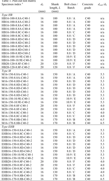
3.2 Element 2 - expanding sleeves model (kHB)

The idealized, empirical model that is proposed to represent the behaviour of the expanding sleeves element is summarized in Table 3 (a), which is determined in conjunction with the notation chart in Fig. 10. The F-δslip element model has tri-linear characteristics, where kxe denotes the

initial stiffness of the element, knorme denotes the normalized initial stiffness of the element, µp and

µu are the strain hardening coefficients, respectively, for the post-limit (kxp) and ultimate (kxu)

stiffness, and Fu _{is the ultimate capacity of the component.}

The proposed model was developed on the basis of experimental pull-out test data. Using the

experimental F-δslip data (obtained from pull-out testing of type HB), a tri-linear curve is used to

simplify and idealise the inherently non-linear behaviour of the element. Fig. 11 presents the F-δslip

data of type HB (for each parameter category), alongside regression analysis with respect to the piecewise three segment linear model. Each parameter category (e.g. HB16-100-8.8-C40) represents the group of repeated pull-out tests whose specimen index was identical in terms of design parameters.

The complete data input for the model is outlined in Table 3 (a), where the quantitative values for knorme, µp, µu and the correspondent force ranges have been determined from the

7

their calculations. The model indexes display the geometrical, mechanical and material properties for appropriate selection in their use. The proposed model varies the strength of the concrete applied to the tube, as well as the size and class of the internal bolt. The tri-linear idealization of the data is deemed as satisfactory in capturing the primary features in the response of the element.

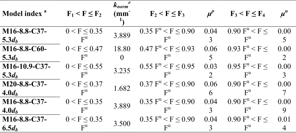
3.3 Element 3 - mechanical anchorage model (kM)

The idealized, empirical model that is proposed to represent the force-slip (F-δslip) behaviour for

the mechanical anchorage element of the EHB system is outlined in Table 3 (b), also determined

in conjunction with Fig. 10. Likewise with the model development of element 2 (kHB), to simplify

non-linear behaviour, a tri-linear curve fit was used in the idealization of the experimental F-δslip

relationship (obtained from pull-out testing of type M). Fig. 12 presents the normalised test data and the idealised element models. The proposed model varies the strength of the concrete infill, the size and class of the internal bolt, and the embedded depth.

3.4 Proposed EHB component method model (kEHB)

It has been stated that three elements contribute to the global deformability curve of the EHB anchored blind-bolt component: namely, the internal bolt, expanding sleeves, and mechanical anchorage. This section proposes an assembly procedure for these constitutive elements in view of

estimating the global force-displacement (F-δglobal) behaviour of the EHB component.

It is proposed to estimate the monotonic tensile response of the EHB component with the use of a massless spring model, formed as shown in Fig. 13. Each spring is characterised by a multi-linear force-displacement relationship (see Section 3.1 to 3.3) and the arrangement of the springs was developed based on experimental observations. The model approximates the behaviour of the

component by placing the expanding sleeves (kHB) and mechanical anchorage (kM) elements in a

parallel arrangement, while in series with the internal bolt elongation (kb) element.

The effective spring constant kEHB is determined on the foundation of basic spring models. This

process is described as having first to express an effective spring for those in parallel (i.e. for kHB

and kM) and then to assemble the combination of the effective parallel spring with that of kb in

series. To illustrate the basic spring formulations, equivalent spring models for parallel and serial configurations are schematically shown in Fig. 14. When the elements are arranged in a parallel configuration, the resulting properties of the assembly can be obtained from the following equations.

𝐹!" =𝐹!"  !+𝐹!"  ! (2)

𝑘=𝑘!+  𝑘! (3)

𝛿!"=min  (𝛿!;𝛿!) (4)

8 𝐹!" =min  (𝐹!"  !;𝐹!"  !) (5)

𝑘 = 1

𝑘!+

1 𝑘!

!!

(6)

𝛿!" =𝛿!+𝛿! (7)

where k is the stiffness and δCd is the deformation capacity. By extending the above formulation

for springs with tri and tetra-linear characteristics, the EHB component method model is calculated accordingly.

Pull-out tests demonstrated that ultimately, the EHB component can develop the full tensile capacity of its internal bolt, exhibiting an ultimate failure mode due to the fracture of its shank (Pitrakkos and Tizani 2013). For the tested geometry, this suggests that the ultimate strength of the

component model (designated Fu) should be taken as equal with the ultimate strength of the

internal bolt, and by no means should the component method model allow for such force levels to be exceeded. This is achieved by imposing the proposed spring arrangement (Fig. 13) which involves kb in a serial configuration. With kb being positioned in series, it is ensured that the

ultimate (and yield) capacity of the internal bolt is captured in the prediction of the component’s

F-δglobal behaviour. A theoretical expression that can be used to estimate the ultimate strength of the

EHB is outlined in Eq. (8), with the resistance function representing a steel failure, where fub is the

bolt ultimate stress and As is the bolt tensile stress area.

𝐹! _=𝑓

!"  𝐴! (8)

For demonstration purposes, an assembled EHB component method model is graphed together with the characteristics of its individual elements in Fig. 15, utilizing the proposed models on the

basis of estimating the experimental F-δglobal behaviour of the pull-out test specimen with index

EHB16-150-8.8D-C40-2. By re-arranging the index in the form of EHB16-5.3db-8.8-C37, it is

recognised that for kb the suitable model would be that of M16 class 8.8 while using batch D

properties, for kHB the index of the model would equate with HB16-8.8-C37, and for kM the

required model index would be M16-8.8-C37-5.3db. The model behaviour presented in Fig. 15 was

determined on the basis of these indexes and it is shown that the equivalent spring model results in

a multi-linear (five piece segment) F-δglobal relationship following the assembly of its constitutive

elements.

4. Comparison of component method model with test results

9

analysis runs up to the deformation capacity of the models, with the charts of Fig. 16 graphing the analysis related to the use of: various bolt batches at benchmark behaviour in charts (a) to (c), a C60 concrete mix in (d), class 10.9 bolts in (e), a larger bolt diameter in (f), and the use of varying embedded depths in (g) and (h).

A penta-linear F-δglobal behaviour is consistently predicted for the component within the range

covered by the investigated parameters; capturing with good agreement the initial, post-limit and ultimate stiffness response. The suggested levels of pre-load forces are found to represent with fair accuracy the initial behaviour of the component for bolts of class 8.8 and of 10.9. Overall, the

model predictions follow the yielding trend of the test data. Using least squares, R2 _{values are also}

reported among the aforementioned charts, with values close to 1 being found; demonstrating a good fit for the component method models.

The term prediction band refers to the region of uncertainties in predicting the response for a single additional observation at each point within a range of independent variable values. It is

computed with respect to a desired confidence level p, whose value is typically chosen to be 95%,

and is represented by two curves lying on opposite sides of the fit. In other words, the prediction band shows the scatter of the data. If many more data points were collected, it is expected that 95%

will fall within the prediction band (Motulsky and Christopoulos 2004). For the F-δglobal behaviour

in this case, the prediction band is the interval of force values, for a given global displacement value, within which 95% of all experimental points in a series of repeated measurements are expected to fall. This suggests, the narrower the interval, the better the predictive nature of the model. It is concluded that at the 95% prediction band level, the EHB component method model predicts with sufficient accuracy the experimental data, taking into account different bolt batches and varying parameters such as concrete strength, bolt class, bolt diameter, and embedded depth. The narrowest prediction band is found to be that of which involves benchmark behaviour (chart c), whereas that possessing the widest band is found to be that of which involves internal bolts of class 10.9 (chart e).

4.1 Influence of excluding pre-load effects

To investigate the influence of excluding the initial level of pre-load forces, the effective stiffness of the proposed EHB component method model (previously shown in Fig. 13) is

determined by modifying element 1 – the tension bolt model, kb. The internal bolt model kb is

modified by transforming the tetra-linear model into a tri-linear model, simply exclusive of its first pre-loading segment (Fig. 17).

In Fig. 18, the global predictions of the EHB component method model, inclusive and exclusive of pre-load effects, are graphed together with relevant experimental data to highlight the effect on the accuracy of the model. The plot emphasizes the significance of including pre-load forces into the assembly procedure; when pre-load effects are excluded, the component method model underestimates the initial and thus also the post-limit stiffness region. It is therefore recommended that pre-load forces are incorporated into the assembly of the proposed model.

5. Component ductility index

10

single components. Therefore, before considering the available rotation capacity of a joint, the available deformation capacity of its components has to be established. It is the purpose of this section to define and classify the deformation capacity of the EHB system with respect to actual (experimental) global data.

In accordance with Kuhlmann et al. (1998), joint components may be classified into three main groups in terms of their force-displacement behaviour:

(1) Components with high ductility, Fig. 19 (a), (2) Components with limited ductility, Fig. 19 (b), (3) Components with brittle failure, Fig. 19 (c).

Components with high ductility present a force-deformation curve that changes from an initial carrying mode into a second carrying mode, which allows increasing deformation with increasing force. The deformation capacity of the component is very high or nearly unlimited, not imposing any bounds on the overall rotation ability of the joint. Components with limited ductility are characterised by a force-deformation curve that exhibits a limit point and a subsequent softening response. In this ductility class, the characteristic available deformation capacity of the component

is defined as the deformation (δCd) belonging to the point at which the force-deformation curves

reach the level of the characteristic force (Fy) again. Brittle failure components behave linearly

until failure, allowing very little deformation before their sudden collapse.

Based on the work by Kuhlmann et al. (1998), Da Silva at al. (2002) proposed a component ductility classification system for joint components with endplate connections. The proposed

classification system involves: (a) a component ductility index, denoted as λ in this paper, and (b)

ductility limits for each component ductility class that was proposed by Kuhlmann et al. (1998).

The component ductility index, λ is determined by the ratio of component collapse to yield

displacement, as expressed in Eq. (9).

𝜆= 𝛥!

𝛥! (9)

And the ductility limits suggested by Da Silva et al. (2002) for the three component ductility classes are:

Class 1: λ≥ 20, for components with high ductility,

Class 2: 3 ≤λ < 20, for components with limited ductility, Class 3: λ < 3, for components with brittle failure.

In a qualitative way, the experimental, non-linear, global force-displacement curves of the EHB component indicate that the component exhibits limited ductility behaviour; justified by the observation of a limit point and subsequent softening with increasing deformation. But to quantitatively classify the EHB component in terms of ductility, in order to calculate its ductility index λ, it is first necessary to define the component yield (Δy_{) and collapse (Δ}u_{) displacement.}

Regarding Δy_{, it is suggested that it is determined at the force level which equates with the elastic}

limit of the internal bolt of the component, denoted as Fy _{and taken as 0.85F}u _{for class 8.8, and} 0.90Fu _{for class 10.9 bolts. On the other hand, Δ}u _{is determined at the point at which the}

force-displacement softening curve reaches the level of the force Fy _{again. Fig. 20 demonstrates the}

11

5.1 Classification using global experimental curve

Using the full non-linear experimental F-δglobal curve, an evaluation of the ductility indexes for

the "EHB in tension" yields the result of Fig. 21, with each index also being summarized in Table 4 alongside the EHB specimen indexes. Based on the ductility classification system suggested in Da Silva et al. (2002) for endplate connection components, it is found that the EHB component can be classified as Class 2 (with limited ductility).

The evaluation includes a variation in parameters related to: concrete strength, fcu; internal bolt

class, fub; internal bolt diameter size, db; and varying embedded depths, demb. The largest index is

exhibited by the component which involved a grade C60 concrete infill, and the lowest ductility index is seen in the case of using class 10.9 bolts. In consideration of over/under strength effects, the component’s benchmark behaviour is investigated by means of using different bolt batches, shown by the first five specimens that are placed on the x-axis. The ductility classification of the component is found to be unaffected among these, demonstrating consistency in the results obtained. Overall, for the tested range, the achieved ductility indexes show that the EHB component is mostly related to the lower bound of the limited ductility class.

For a clearer interpretation of the influence that the varied parameters have on the ductility index of the EHB component, the determined indexes are presented in the form of ductility index

charts in Fig. 22. The format of the ductility index charts involve λ on the y-axis, and on the x-axis

of the charts, it is the appropriate variable that represents the variation in parameter that is graphed

(e.g. fcu for variation in compressive strength). The charts involve mean values on both axes, where

the values along the x-axis were determined based on actual material properties that were involved in the pull-out testing of type EHB. An overall examination of Fig. 22 shows that:

(1) an increase in the compressive strength of the concrete infill results in a higher ductility index, but still falling within the boundary of the limited ductility class, Fig. 22 (a);

(2) when a variation in bolt class of 8.8 to 10.9 is considered, the ductility index of the component reduces with respect to the latter class, involving a transition from limited ductility towards brittle behaviour, Fig. 22 (b);

(3) an increase in bolt diameter size results in a lower ductility index, but still falling within the boundary of the limited ductility class, Fig. 22 (c).

6. Conclusions

Continuing research at the University of Nottingham has identified a moment transmitting configuration for bolted connections to tubular steel profiles. The bolted configuration comprises tubes that are filled with concrete, together with connections that utilise modified blind-bolts with headed anchors attached to their ends. It has been stated that the application of the component-based approach to the design of the proposed connection technology is not possible. The method is limited due to insufficient knowledge of the behaviour of two basic joint components: 1) the "tube face in bending" and 2) the "bolt in tension". This paper has described a component method model for the response of the latter basic joint component, i.e. for the behaviour of the "bolt in tension" component.

12

shank with consideration of pre-load effects, ii) the slip of its expanding sleeves element, and iii) the slip of its headed anchorage element. The model was developed using the principles of the component method – applied in structural joint modelling – where the unknown mechanical properties of the component were characterised and further idealised in order to establish the constitutive models.

The validity of the model was assessed against experimental data with respect to the connector’s response as a whole, and the model was found to provide reliable predictions for the considered range of parameters; with the model results satisfying the 95% prediction band. The degree of accuracy of the proposed model was found to heavily rely on the input of an appropriate model for its pre-loading condition. Therefore, the use of the idealised characteristics for the connector’s constituent parts, combined with the procedure proposed for their assembly, demonstrates the successful application of the scientific component method for the studied joint component. The bolt model is thus considered suitable for use in component connection models – within the range of parameters covered – and it can be applied in a global mechanical model that is to predict the moment-rotation characteristics of the overall connection.

Acknowledgments

The authors would like to acknowledge the support of TATA Steel and Lindapter International for the research work presented in this paper. Gratitude is expressed to Mr Trevor Mustard and Mr Andrew Orton, of TATA Steel, and Mr Neil F. Gill, of Lindapter International. The first author is also thankful for the support provided by the EPSRC (DTA) and Corus Tubes for his doctoral research studies.

References

Barron, J. (1998), Handbook of bolts and bolted joints: Computing the stiffness of a fastener, CRC Press, Marcel Dekker, New York.

Bickford, J.H. (2008), "Introduction to the Design and Behavior of Bolted Joints , Fourth Edition , Non-Gasketed Joints, Taylor & Francis Group.".

British Steel (1997), SHS Jointing: Flowdrill & Hollobolt. British Steel Plc,

BSI (2001), ISO metric precision hexagon bolts, screws and nuts - Specification, BS 3692:2001, London. BSI (2009), Mechanical properties of fasteners made of carbon steel and alloy steel, Part 1: Bolts, screws

and studs with specified property classes - Coarse thread and fine pitch thread, BS EN ISO 898-1:2009,

British Standards Institution, London.

CEN (2010a), Eurocode 3: Design of steel structures – Part 1-1: General rules and rules for buildings, BS EN 1993-1-1:2005, British Standards Institution (Incorporating Corrigenda).

CEN (2010b), Eurocode 3: Design of steel structures – Part 1-8: Design of joints, BS EN 1993-1-8:2005, British Standards Institution (Incorporating Corrigenda).

Da Silva, L.S., Santiago, A. and Vila Real, P. (2002), "Post-limit stiffness and ductility of end-plate beam-to-column steel joints", Computers & Structures. 80(5-6), 515-531.

ECCS (1986), Technical Committee 1: structural safety and loadings: technical working group 1.3: seismic design, recommended testing procedure for assessing the behaviour of structural steel elements under

cyclic loads.

13

of Conf. on Mechanics of Structures & Materials, Bridge and Foster (eds.), Balkema, Rotterdam,

Netherlands, December, pp. 309-314.

Gardner, A.P. and Goldsworthy, H.M. (2005), "Experimental investigation of the stiffness of critical components in a moment-resisting composite connection", Journal of Constructional Steel Research.61(5), 709-726.

Flowdrill Product Brochure, Available at: http://www.flowdrill.com (last accessed: 25 Sep 2013). HuckBOM Product Brochure, Available at: http://www.afshuck.net/ (last accessed: 25 Sep 2013).

Kuhlmann, U., Davison, J.B. and Kattner, M. (1998), "Structural systems and rotation capacity", In: Proceedings of COST C1 conference on Control of the Semi-rigid Behaviour of Civil Engineering

Structural Connections, Université de Liège, Belgium, September, pp. 167-176.

Lindapter (2013a), Type HB - Hollo-Bolt®, Lindapter International, UK. Lindapter (2013b), Type LB2 - Lindibolt® _{2, Lindapter International, UK.}

Molabolt Product Brochure, Available at: http://www.molabolt.co.uk (last accessed: 25 Sep 2013).

Motulsky, H. and Christopoulos, A. (2004), Fitting models to biological data using linear and nonlinear

regression: a practical guide to curve fitting, Oxford University Press, USA.

ONESIDE Product Brochure, Available at: http://www.ajaxfast.com.au (last accessed: 25 Sep 2013). Pitrakkos, T. (2012), The Tensile Stiffness of a Novel Anchored Blind-bolt Component for Moment-resisting

Connections to Concrete-filled Hollow Sections, PhD Thesis, University of Nottingham, UK.

Pitrakkos, T. and Tizani, W. (2013), "Experimental behaviour of a novel anchored blind-bolt in tension",

Engineering Structures. 49(0), 905-919.

SCI/BCSA (2002), Joints in steel construction: Simple Connections, Steel Construction Institute (SCI) & British Constructional Steelwork Association (BCSA), Ascot.

SCI/BCSA (2011), Joints in steel construction: Simple joints to Eurocode 3, Steel Construction Institute (SCI) & British Constructional Steelwork Association (BCSA), Ascot.

The Blind Bolt Product Brochure, Available at: http://www.blindbolt.co.uk (last accessed: 25 Sep 2013). Tizani, W., Al-Mughairi, A., Owen, J.S. and Pitrakkos, T. (2013a), "Rotational stiffness of a blind-bolted

connection to concrete-filled tubes using modified Hollo-bolt", Journal of Constructional Steel Research.

80(0), 317-331.

Tizani, W., Wang, Z.Y. and Hajirasouliha, I. (2013b), "Hysteretic performance of a new blind bolted connection to concrete filled columns under cyclic loading: An experimental investigation", Engineering

Structures. 46(0), 535-546.

Wang, J.-F., Han, L.-H. and Uy, B. (2009), "Behaviour of flush end plate joints to concrete-filled steel tubular columns", Journal of Constructional Steel Research. 65(4), 925-939.

Wang, J. and Spencer Jr, B.F. (2013), "Experimental and analytical behavior of blind bolted moment connections", Journal of Constructional Steel Research. 82(0), 33-47.

Wardenier, J., Packer, J., Zhao, X-L and Vegte, G.J. van der (2010), Hollow sections in structural

applications (2nd edition), CIDECT, Geneva, Switzerland.

Yao, H., Goldsworthy, H. and Gad, E. (2008) "Experimental and numerical investigation of the tensile behavior of blind-bolted T-Stub connections to concrete-filled circular columns", ASCE Journal of

14

Specimen index a _d

b

(mm)

Shank length, L

(mm)

Bolt class / Batch

Concrete grade

demb /db

Type HB

HB16-100-8.8A-C40-1 16 100 8.8 / A C40 n/a

HB16-100-8.8A-C40-2 16 100 8.8 / A C40 n/a

HB16-100-8.8A-C40-3 16 100 8.8 / A C40 n/a

HB16-100-8.8A-C40-4 16 100 8.8 / A C40 n/a

HB16-100-8.8C-C40-1 16 100 8.8 / C C40 n/a

HB16-100-8.8C-C40-2 16 100 8.8 / C C40 n/a

HB16-100-8.8D-C40-1 16 100 8.8 / D C40 n/a

HB16-100-8.8D-C40-2 16 100 8.8 / D C40 n/a

HB16-100-8.8D-C40-3 16 100 8.8 / D C40 n/a

HB16-100-8.8D-C60-1 16 100 8.8 / D C60 n/a

HB16-100-8.8D-C60-2 16 100 8.8 / D C60 n/a

HB16-100-10.9E-C40-1 16 100 10.9 / E C40 n/a

HB16-100-10.9E-C40-2 16 100 10.9 / E C40 n/a

HB20-120-8.8F-C40-1 20 120 8.8 / F C40 n/a

HB20-120-8.8F-C40-2 20 120 8.8 / F C40 n/a

Type M

M16-150-8.8A-C40-1 16 150 8.8 / A C40 5.3

M16-150-8.8A-C40-2 16 150 8.8 / A C40 5.3

M16-150-8.8D-C40-1 16 150 8.8 / D C40 5.3

M16-150-8.8D-C40-2 16 150 8.8 / D C40 5.3

M16-150-8.8D-C40-3 16 150 8.8 / D C40 5.3

M16-150-8.8D-C60-1 16 150 8.8 / D C60 5.3

M16-150-8.8D-C60-2 16 150 8.8 / D C60 5.3

M16-150-10.9E-C40-1 16 150 10.9 / E C40 5.3

M16-150-10.9E-C40-2 16 150 10.9 / E C40 5.3

M20-150-8.8F-C40-1 20 150 8.8 / F C40 4.0

M20-150-8.8F-C40-2 20 150 8.8 / F C40 4.0

M16-130-8.8C-C40-1 16 130 8.8 / C C40 4.0

M16-130-8.8C-C40-2 16 130 8.8 / C C40 4.0

M16-170-8.8B-C40-1 16 170 8.8 / B C40 6.5

M16-170-8.8B-C40-2 16 170 8.8 / B C40 6.5

Type EHB

EHB16-150-8.8A-C40-1 16 150 8.8 / A C40 5.3

EHB16-150-8.8C-C40-1 16 150 8.8 / C C40 5.3

EHB16-150-8.8D-C40-1 16 150 8.8 / D C40 5.3

EHB16-150-8.8D-C40-2 16 150 8.8 / D C40 5.3

EHB16-150-8.8D-C40-3 16 150 8.8 / D C40 5.3

EHB16-150-8.8D-C60-1 16 150 8.8 / D C60 5.3

EHB16-150-8.8D-C60-2 16 150 8.8 / D C60 5.3

EHB16-150-10.9E-C40-1 16 150 10.9 / E C40 5.3

EHB16-150-10.9E-C40-2 16 150 10.9 / E C40 5.3

EHB20-150-8.8F-C40-1 20 150 8.8 / F C40 4.0

EHB20-150-8.8F-C40-2 20 150 8.8 / F C40 4.0

EHB16-130-8.8C-C40-1 16 130 8.8 / C C40 4.0

EHB16-130-8.8C-C40-2 16 130 8.8 / C C40 4.0

EHB16-170-8.8B-C40-1 16 170 8.8 / B C40 6.5

EHB16-170-8.8B-C40-2 16 170 8.8 / B C40 6.5

a _{(1)-(2)-(3)-(4)-(5): (1) type of fastener (HB, M, or EHB) & internal bolt diameter, d}

[image:14.595.74.432.125.722.2]

15

0.030 0.883

A 915 1020 0.897

A 917 1026 0.894

A 876 983 0.891

B 725 900 0.806

C 874 981 0.891

C 872 981 0.889

D 864 950 0.910

D 832 926 0.898

D 832 924 0.900

D 814 922 0.883

F 785 935 0.840

10.9 E 1067 1116 0.956

0.005 0.952

E 1094 1146 0.954

E 1091 1154 0.946

[image:15.595.73.350.92.311.2]

E 1092 1147 0.952

Table 3. Tri-linear idealised force-slip models for elements 2 and 3

(a) kHB (stiffness related to expanding sleeves element of EHB component)

Model index

a

F

1

< F

≤

F

2

k

norme

(mm

-1

₎

F

2

< F

≤

F

3

µ

p

_F

3

< F

≤

F

4

µ

u

HB16-8.8-C37

0 < F ≤ 0.60

F

u

1.091

0.60 F

u

< F ≤ 0.90

F

u

0.28

9

0.90 F

u

< F ≤

F

u

0.03

2

HB16-8.8-C60

0 < F ≤ 0.55

F

u

3.056

0.55 F

u

< F ≤ 0.92

F

u

0.17

5

0.92 F

u

< F ≤

F

u

0.08

0

HB16-10.9-C37

0 < F ≤ 0.55

F

u

1.000

0.55 F

u

< F ≤ 0.95

F

u

0.16

3

0.95 F

u

< F ≤

F

u

0.01

8

HB20-8.8-C37

0 < F ≤ 0.25

F

u

1.114

0.25 F

u

< F ≤ 0.68

F

u

0.29

8

0.68 F

u

< F ≤

F

u

0.08

7

(b) kM (stiffness related to mechanical anchorage element of EHB component)

Model index

a

F

1

< F

≤

F

2

k

norme

(mm

-1

₎

F

2

< F

≤

F

3

µ

p

_F

3

< F

≤

F

4

µ

u

M16-8.8-C37-5.3

d

b

0 < F ≤ 0.35

F

u

3.889

0.35 F

u

_{< F ≤ 0.90}

F

u

0.04

3

0.90 F

u

_{< F ≤}

F

u

0.00

5

M16-8.8-C60-5.3

d

b

0 < F ≤ 0.47

F

u

18.80

0

0.47 F

u

< F ≤ 0.93

F

u

0.06

5

0.93 F

u

< F ≤

F

u

0.00

2

M16-10.9-C37-5.3

d

b

0 < F ≤ 0.55

F

u

3.235

0.55 F

u

< F ≤ 0.95

F

u

0.03

2

0.95 F

u

< F ≤

F

u

0.00

3

M20-8.8-C37-4.0

d

b

0 < F ≤ 0.37

F

u

1.682

0.37 F

u

< F ≤ 0.90

F

u

0.06

6

0.90 F

u

< F ≤

F

u

0.00

7

M16-8.8-C37-4.0

d

b

0 < F ≤ 0.35

F

u

3.889

0.35 F

u

< F ≤ 0.90

F

u

0.04

3

0.90 F

u

< F ≤

F

u

0.00

9

M16-8.8-C37-6.5

d

b

0 < F ≤ 0.35

F

u

3.500

0.35 F

u

< F ≤ 0.90

F

u

0.04

3

0.90 F

u

< F ≤

F

u

0.01

4

[image:15.595.76.548.541.753.2]

[image:16.595.76.382.162.366.2]

16 Table 4. Ductility index ratio

Specimen index a Δy

(mm)

Δu

(mm)

λ

EHB16-150-8.8A-C40-1 0.88 6.49 7.4

EHB16-150-8.8C-C40-1 0.81 6.34 7.9

EHB16-150-8.8D-C40-1 0.59 7.47 12.7

EHB16-150-8.8D-C40-2 0.59 6.51 11.0

EHB16-150-8.8D-C40-3 0.52 7.08 13.6

EHB16-150-8.8D-C60-1 0.37 6.16 16.7

EHB16-150-8.8D-C60-2 0.44 6.78 15.6

EHB16-150-10.9E-C40-1 0.88 4.52 5.2

EHB16-150-10.9E-C40-2 0.98 4.51 4.6

EHB20-150-8.8F-C40-1 1.07 9.90 9.2

EHB20-150-8.8F-C40-2 1.10 9.27 8.4

EHB16-130-8.8C-C40-1 0.76 6.23 8.2

EHB16-130-8.8C-C40-2 0.84 6.47 7.7

EHB16-170-8.8B-C40-1 1.41 6.62 4.7

EHB16-170-8.8B-C40-2 1.28 6.52 5.1

17

[image:17.595.85.513.100.282.2]

(a) Five part HB before tightening (b) Connection to tubular profile using the HB

Fig. 1. The Lindapter Hollo-bolt® _{(HB) (Lindapter 2013a)}

Fig. 2. Proposed blind-bolted moment transmitting connection M

a

c

d

a. Extended Hollo-bolts b. Endplate

c. I-beam section d. Concrete-filled tube

[image:17.595.83.306.146.277.2]

18

[image:18.595.94.487.90.289.2]

(a) (b)

Fig. 3. The innovative Extended Hollo-bolt (EHB) blind-bolt and its constituent elements

Fig. 4. Basic joint components that contribute to rotational stiffness of connection

anchor head

mechanical anchorage

3

expanding sleeves

2

internal bolt elongation

1

joint members

M

Z

X

Υ

Basic joint components: X. Bolts (EHB) in tension

[image:18.595.119.473.335.524.2]

[image:19.595.186.514.87.290.2] [image:19.595.70.521.87.746.2]

19 Fig. 5. Type of fastener or element tested

Fig. 6. Pull-out test setup

d_emb L

L

M

HB

EHB

W

δ_global

δ_slip

Loaded end

Unloaded end F loading frame

20 (a) Class 8.8

[image:20.595.79.320.96.457.2]

(b) Class 10.9

Fig. 7. Idealised (tetra-linear) internal bolt model

0 20 40 60 80 100

0 0.5 1 1.5 2 2.5 3 3.5 4

F

or

ce

(k

N

)

Bolt elongation, δ_b (mm)

0 20 40 60 80 100 120 140 160

0 0.5 1 1.5 2 2.5 3 3.5 4

F

or

ce

(k

N

)

Bolt elongation, δ_b (mm)

k_xe = E_b A_s / L_b k_xp= 0.050 k_xe

0.15Fu 1000 k_xe

k_x = 0.010 k_x

0.85F

k_xe = E_b A_s / L_b k_xp= 0.100 k_xe

k_xu= 0.015 k_xe

Fu

0.25Fu 1000 k_xe

21 Fig. 8. Effective length, Lb for internal bolt of EHB component

(a) M16 class 8.8

(b) M16 class 10.9

(c) M20 class 8.8

Fig. 9. Comparison of element 1 (kb) models with experimental data Lb

W

0 40 80 120 160 200 240

0 1 2 3 4 5 6 7 8 9 10

F

or

ce

(k

N

)

Bolt elongation, δb (mm)

EHB16-150-8.8D-C40-1 Bolt Model (M16 gr.8.8)

0 40 80 120 160 200 240

0 1 2 3 4 5 6 7 8 9 10

F

or

ce

(k

N

)

Bolt elongation, δb (mm)

EHB16-150-10.9E-C40-1 Bolt Model (M16 gr.10.9)

0 40 80 120 160 200 240

0 1 2 3 4 5 6 7 8 9 10

F

or

ce

(k

N

)

Bolt elongation, δb (mm)

EHB20-150-8.8F-C40-1 Bolt Model (M20 gr.8.8)

R2_=0.987

R2_=0.929

22 Fig. 10. Notation chart for kHB and kM

(a) HB16-8.8-C37 (b) HB16-8.8-C60

(c) HB16-10.9-C37 (d) HB20-8.8-C37

Fig. 11. Normalised experimental data and idealised models for kHB 0 20 40 60 80 100 120

0 2 4 6 8

F or ce (k N )

δ_slip (mm)

0.0 0.2 0.4 0.6 0.8 1.0 1.2

0 1 2 3 4 5 6 7

F

/ F

te

st,max

δ_slip (mm)

HB16-100-8.8-C40

Model (idealised) _0.0 0.2

0.4 0.6 0.8 1.0 1.2

0 1 2 3 4 5 6 7

F

/ F

te

st,max

δ_slip (mm)

HB16-100-8.8-C60 Model (idealised) 0.0 0.2 0.4 0.6 0.8 1.0 1.2

0 1 2 3 4 5 6 7

F

/ F

te

st,max

δslip (mm)

HB16-100-10.9-C40

Model (idealised) _0.0 0.2

0.4 0.6 0.8 1.0 1.2

0 1 2 3 4 5 6 7

F

/ F

te

st,max

δslip (mm)

HB20-120-8.8-C40 Model (idealised)

R2 _{= 0.924 R}2 _{= 0.928}

R2 _{= 0.879 R}2 _{= 0.889}

k_xe=k_norme Fu

k_xp=µpk_xe

k_xu=µu k_xe

23

(a) M16-8.8-C37-5.3db (b) M16-8.8-C60-5.3db

(c) M16-10.9-C37-5.3db (d) M20-8.8-C37-4.0db

(e) M16-8.8-C37-4.0db (f) M16-8.8-C37-6.5db

Fig. 12. Normalised experimental data and idealised models for kM 0.0

0.2 0.4 0.6

0 2 4 6 8 10 12 14

F

/ F

te

δslip (mm)

M16-150-8.8-C40

Model (idealised) _0.0 0.2

0.4 0.6

0 2 4 6 8 10 12 14

F

/ F

te

δslip (mm)

M16-150-8.8-C60 Model (idealised) 0.0 0.2 0.4 0.6 0.8 1.0 1.2

0 2 4 6 8 10 12 14

F

/ F

te

st,max

δ_slip (mm)

M16-150-10.9-C40

Model (idealised) _0.0 0.2

0.4 0.6 0.8 1.0 1.2

0 2 4 6 8 10 12 14

F

/ F

te

st,max

δ_slip (mm)

M20-150-8.8-C40 Model (idealised) 0.0 0.2 0.4 0.6 0.8 1.0 1.2

0 2 4 6 8 10 12 14

F

/ F

te

st,max

δ_slip (mm)

M16-130-8.8-C40

Model (idealised) _0.0 0.2

0.4 0.6 0.8 1.0 1.2

0 2 4 6 8 10 12 14

F

/ F

te

st,max

δ_slip (mm)

M16-170-8.8-C40 Model (idealised)

R2 _{= 0.867 R}2 _{= 0.681}

R2 _{= 0.807 R}2 _{= 0.860}

24 Fig. 13. Equivalent spring (component) model for EHB anchored blind-bolt

(a) Parallel configuration (b) Serial configuration

Fig. 14. Assembly of springs

Fig. 15. Spring characteristics and assembled component model

k

M

k

HB

k

b

k

EHB 1

2 3

-10 10 30 50 70 90 110 130 150

0 0.5 1 1.5 2 2.5 3 3.5 4

F

δ

FRd

δCd

1 2

1

2 F

0 50 100 150 200 250

0 0.5 1 1.5 2 2.5 3 3.5 4

F

δ

FRd

δCd

3

4

3 4 F

-40 10 60 110 160

0 1 2 3 4 5 6 7 8 9 10

F

or

ce

(k

N

)

Displacement (mm)

kb kHB kM

Experimental Global - full bolt Model

kM

25

(a) (b)

(c) (d)

(e) (f)

(g) (h)

Fig. 16. Comparison of component method model predictions with experimental data 0 20 40 60 80 100 120

0 0.5 1 1.5 2 2.5 3 3.5 4 4.5

F

or

ce

(k

N

δglobal (mm)

EHB16-150-8.8A-C40-1 95% Prediction Band EHB Spring Model

0 20 40 60 80 100 120

0 0.5 1 1.5 2 2.5 3 3.5 4 4.5

F

or

ce

(k

N

δglobal (mm)

EHB16-150-8.8C-C40-1 95% Prediction Band EHB Spring Model

0 20 40 60 80 100 120 140 160 180

0 0.5 1 1.5 2 2.5 3 3.5 4 4.5

F or ce (k N )

δglobal (mm)

EHB16-150-8.8D-C40-2 95% Prediction Band EHB Spring Model

0 20 40 60 80 100 120 140 160 180

0 0.5 1 1.5 2 2.5 3 3.5 4 4.5

F or ce (k N )

δglobal (mm)

EHB16-150-8.8D-C60-1 95% Prediction Band EHB Spring Model

0 20 40 60 80 100 120 140 160 180 200

0 0.5 1 1.5 2 2.5

F or ce (k N )

δ_global (mm)

EHB16-150-10.9E-C40-1 95% Prediction Band

EHB Spring Model 20 40 ₀

60 80 100 120 140 160 180 200 220 240

0 0.5 1 1.5 2 2.5 3 3.5 4 4.5 5 5.5

F or ce (k N )

δ_global (mm)

EHB20-150-8.8F-C40-1 95% Prediction Band EHB Spring Model

0 20 40 60 80 100 120 140 160 180

0 0.5 1 1.5 2 2.5 3 3.5 4 4.5

F or ce (k N )

δ_global (mm)

EHB16-130-8.8C-C40-1 95% Prediction Band EHB Spring Model

0 20 40 60 80 100 120 140 160 180

0 0.5 1 1.5 2 2.5 3 3.5 4 4.5

F or ce (k N )

δ_global (mm)

EHB16-170-8.8B-C40-2 95% Prediction Band EHB Spring Model

R2 _{=0.985 R}2 _=0.983

R2 _{=0.991 R}2 _=0.990

R2 _{=0.951 R}2 _=0.988

26 Fig. 17. Modified internal bolt model (kb) to investigate effect of excluding pre-load (class 8.8 bolts)

Fig. 18. Component model predictions including/excluding pre-load effects (class 8.8 bolts)

(a) High ductility (b) Limited ductility (c) Brittle failure

Fig. 19. Ductility classes for joint components

0 20 40 60 80 100

0 0.5 1 1.5 2 2.5 3 3.5 4

F

or

ce

(k

N

)

Bolt elongation, δ_b (mm)

0 20 40 60 80 100 120 140

0 0.1 0.2 0.3 0.4 0.5 0.6 0.7 0.8 0.9 1

F

or

ce

(k

N

)

δ_global (mm)

EHB16-150-8.8D-C40-2 incl preload

excl preload

δ F

δ δ

F F

δCd Fy

Fy

δCd

δCd Fy

k_xe = E_b A_s / L_b k_xp= 0.050 k_xe

k_x = 0.010 k_x

27 Fig. 20. Component yield and collapse displacement

Fig. 21. Component ductility classification (using global experimental curve)

(a) Δy Δu 0 50 100

0 1 2 3 4 5 6 7 8

F

or

ce

(k

δglobal (mm)

EHB16-150-8.8D-C40-2 Limited High 0 4 8 12 16 20 24 E H B16-150-8.8A -E H B16-150-8.8C-E H B16-150-8.8D -E H B16-150-8.8D -E H B16-150-8.8D -E H B16-150-8.8D -E H B16-150-8.8D -E H B16-150-10.9E -E H B16-150-10.9E -E H B20-150-8.8F -E H B20-150-8.8F -E H B16-130-8.8C-E H B16-130-8.8C-E H B16-170-8.8B-E H B16-170-8.8B-D u cti li ty i n d ex, λ Specimen index 0 4 8 12 16 20

35 40 45 50 55 60

D u cti li ty i n d ex, λ

28 (b)

[image:28.595.96.323.89.390.2]

(c)

Fig. 22. Component ductility index charts 0

4 8

800 900 1000 1100 1200

D

u

cti

li

ty i

fub (MPa)

0 4 8 12 16 20

12 16 20 24

D

u

cti

li

ty i

n

d

ex,

λ

db (mm) Class 8.8