Bayesian integration of flux tower data into a process based simulator for quantifying uncertainty in simulated output

https://doi.org/10.5194/gmd-11-83-2018

© Author(s) 2018. This work is distributed under the Creative Commons Attribution 3.0 License.

Bayesian integration of flux tower data into a process-based

simulator for quantifying uncertainty in simulated output

Rahul Raj, Christiaan van der Tol, Nicholas Alexander Samuel Hamm, and Alfred Stein

Faculty of Geo-Information Science and Earth Observation (ITC), University of Twente, P.O. Box 217, 7514 AE Enschede, the Netherlands

Correspondence:Rahul Raj ([email protected], [email protected]) Received: 15 August 2016 – Discussion started: 12 October 2016

Revised: 7 November 2017 – Accepted: 17 November 2017 – Published: 9 January 2018

Abstract.Parameters of a process-based forest growth sim-ulator are difficult or impossible to obtain from field ob-servations. Reliable estimates can be obtained using cali-bration against observations of output and state variables. In this study, we present a Bayesian framework to cali-brate the widely used process-based simulator Biome-BGC against estimates of gross primary production (GPP) data. We used GPP partitioned from flux tower measurements of a net ecosystem exchange over a 55-year-old Douglas fir stand as an example. The uncertainties of both the Biome-BGC pa-rameters and the simulated GPP values were estimated. The calibrated parameters leaf and fine root turnover (LFRT), ra-tio of fine root carbon to leaf carbon (FRC : LC), rara-tio of carbon to nitrogen in leaf (C : Nleaf), canopy water intercep-tion coefficient (Wint), fraction of leaf nitrogen in RuBisCO (FLNR), and effective soil rooting depth (SD) characterize the photosynthesis and carbon and nitrogen allocation in the forest. The calibration improved the root mean square er-ror and enhanced Nash–Sutcliffe efficiency between simu-lated and flux tower daily GPP compared to the uncalibrated Biome-BGC. Nevertheless, the seasonal cycle for flux tower GPP was not reproduced exactly and some overestimation in spring and underestimation in summer remained after cali-bration. We hypothesized that the phenology exhibited a sea-sonal cycle that was not accurately reproduced by the sim-ulator. We investigated this by calibrating the Biome-BGC to each month’s flux tower GPP separately. As expected, the simulated GPP improved, but the calibrated parameter values suggested that the seasonal cycle of state variables in the sim-ulator could be improved. It was concluded that the Bayesian framework for calibration can reveal features of the modelled

physical processes and identify aspects of the process simu-lator that are too rigid.

1 Introduction

Forest ecosystems play an important role in the global car-bon cycle by controlling the atmospheric CO2level. Knowl-edge of gross primary production (GPP) for forest ecosys-tems is indispensable for the estimation of forest carbon stor-age. GPP is the first entry of atmospheric carbon into the for-est ecosystem via photosynthesis. Process-based forfor-est sim-ulators (PBSs) evaluate forest ecosystem activity by simulat-ing different physiological plant responses to climatic condi-tions, atmospheric properties and plant structures (Constable and Friend, 2000; Running, 1994).

Simulating a PBS requires input parameters that distin-guish different vegetation types by their physiological and morphological characteristics. Implementation of a PBS for specific sites is complicated by the large number of param-eters for plants, the soil and the atmosphere. Field measure-ments of PBS parameters are difficult or impossible to obtain, leading to incomplete knowledge of site-specific parameters for the occurring species. In practice, practitioners often rely on the literature for values of the PBS parameters (Hartig et al., 2012; Mäkelä et al., 2000).

the parameters and the simulated outputs. Quantification of uncertainty is important for both scientific and practical pur-poses (Hamm et al., 2015b; Verstegen et al., 2014; He et al., 2014; Bastin et al., 2013).

A Bayesian framework provides a coherent method for calibrating a PBS (van Oijen et al., 2011; Reinds et al., 2008; van Oijen et al., 2005) and involves the identification of un-certainty in the parameters from the available information. This uncertainty is expressed as the prior probability distri-butions of the parameters. Independent observations of the variables corresponding to the PBS outputs (e.g. GPP) are used to update the prior probability distributions by means of Bayes’ rule. This updating generates the posterior probabil-ity distributions of the parameters, which can be summarized as medians and 95 % credible intervals as the quantification of uncertainty. Hence, a Bayesian framework combines prior probability distributions of the parameters and the observa-tions to quantify uncertainty in the parameters and the PBS outputs.

In this study, a widely used simulator, Biome-BGC (Thornton, 1998), was calibrated in a Bayesian framework for a single output variable, GPP. A systematic search of the literature was used to construct the prior probability distri-butions on the Biome-BGC parameters (Raj et al., 2014). A time series of daily flux tower GPP, partitioned from the flux tower measurements of net ecosystem exchange (NEE), provided independent GPP observations (Raj et al., 2016). We used flux tower GPP to update the priors of Biome-BGC parameters. In principle, NEE data could be used alone to calibrate Biome-BGC, where NEE is derived as the dif-ference between the GPP and ecosystem respiration (Reco). Hence, a calibration of Biome-BGC using NEE data only ensures the accuracy of difference between GPP and Reco (Mitchell et al., 2011). The accuracy of simulated GPP can not be achieved using the NEE data alone. Our study fo-cused on achieving the accuracy of simulated first entry of atmospheric carbon, i.e. GPP, into the ecosystem. Therefore, we used partitioned flux tower GPP data to calibrate Biome-BGC.

Biome-BGC simulates GPP at a daily time step and it up-dates its memory between days (Thornton, 2010; White et al., 2000). This memory corresponds to the mass (amount of car-bon) stored in different components of the vegetation, litter, and soil. The update of memory is directly related to the sea-sonal development of the state variables such as carboxyla-tion capacity (Vcmax) that in turn controls the seasonality of simulated GPP. Input parameters are important to control the seasonality of the state variables and thus of GPP. Biome-BGC accepts constant values of the input parameters during a simulation over the entire study period. We hypothesized that the seasonal cycle of GPP was not accurately captured by the constant (time-invariant) parameters and that their temporal variations could probably improve the seasonal cycle of GPP. We, therefore, further investigated if the temporal variation in

the input parameters could be captured by means of Bayesian calibration.

The objective of this study was to quantify the uncertainty in Biome-BGC input parameters and simulated GPP by in-tegrating flux tower GPP into Biome-BGC in a Bayesian framework. We obtained the posterior Biome-BGC param-eters (a) by calibrating the Biome-BGC to the data of en-tire study period (growing season) and (b) by calibrating the Biome-BGC to 1 month of GPP data and repeating the cali-bration for all months in the growing season. The main nov-elty of this paper is the presentation of a Bayesian framework for Biome-BGC parameter estimation. The simulator itself is left unaltered. Additionally, investigation of temporal varia-tion in Biome-BGC input parameters would also reinforce the reconsideration of the assumption of constant parameters of other process-based simulators for photosynthesis.

2 Site description

Calibration of Biome-BGC was performed at the Speulder-bos Forest site, which is located at 52◦1500800N, 05◦4102500E within a large forested area in the Netherlands. There is a flux tower within a dense 2.5 ha Douglas fir stand, which is a type of evergreen needleleaf species. The stand was planted in 1962. The vegetation, soil, and climate of this site have been thoroughly described elsewhere (Raj et al., 2014; Su et al., 2009; van Wijk et al., 2001; Steingrover and Jans, 1994).

3 Methods

3.1 Data and simulators

3.1.1 The Biome-BGC simulator

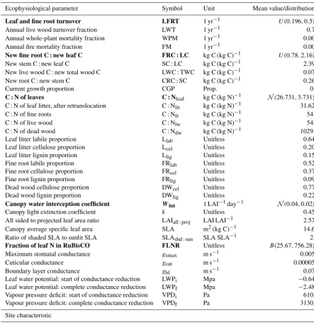
Table 1. The 35 ecophysiological parameters needed to run Biome-BGC for Douglas fir (evergreen needleleaf species). Mean val-ues/distributions were taken from Raj et al. (2014). The ecophysiological parameters highlighted in bold and the effective soil rooting depth were included in a Bayesian calibration.

Ecophysiological parameter Symbol Unit Mean value/distribution∗

Leaf and fine root turnover LFRT 1 yr−1 U (0.196,0.5)∗

Annual live wood turnover fraction LWT 1 yr−1 0.70

Annual whole-plant mortality fraction WPM 1 yr−1 0.005

Annual fire mortality fraction FM 1 yr−1 0.005

New fine root C : new leaf C FRC : LC kg C (kg C)−1 U (0.78,2.16)∗

New stem C : new leaf C SC : LC kg C (kg C)−1 2.391

New live wood C : new total wood C LWC : TWC kg C (kg C)−1 0.071

New root C : new stem C CRC : SC kg C (kg C)−1 0.262

Current growth proportion CGP Prop. 0.5

C : N of leaves C : Nleaf kg C (kg N)−1 N(26.731,3.731)∗

C : N of leaf litter, after retranslocation C : Nlit kg C (kg N)−1 31.625

C : N of fine roots C : Nfr kg C (kg N)−1 54.8

C : N of live wood C : Nlw kg C (kg N)−1 54.8

C : N of dead wood C : Ndw kg C (kg N)−1 1029.5

Leaf litter labile proportion Llab Unitless 0.644

Leaf litter cellulose proportion Lcel Unitless 0.201

Leaf litter lignin proportion Llig Unitless 0.155

Fine root labile proportion FRlab Unitless 0.527

Fine root cellulose proportion FRcel Unitless 0.378

Fine root lignin proportion FRlig Unitless 0.095

Dead wood cellulose proportion DWcel Unitless 0.772

Dead wood lignin proportion DWlig Unitless 0.228

Canopy water interception coefficient Wint 1 LAI−1day−1 N(0.04,0.02)∗

Canopy light extinction coefficient k Unitless 0.453

All sided to projected leaf area ratio LAIall:proj LAI LAI−1 2.572

Canopy average specific leaf area SLA m2(kg C)−1 14.65

Ratio of shaded SLA to sunlit SLA SLAshd:sun SLA SLA−1 2.0

Fraction of leaf N in RuBisCO FLNR Unitless B(25.67,756.28)∗

Maximum stomatal conductance gsmax m s−1 0.0051

Cuticular conductance gcut m s−1 0.000051

Boundary layer conductance gbl m s−1 0.075

Leaf water potential: start of conductance reduction LWPi Mpa −0.647 Leaf water potential: complete conductance reduction LWPf Mpa −2.487

Vapour pressure deficit: start of conductance reduction VPDi Pa 610.0

Vapour pressure deficit: complete conductance reduction VPDf Pa 3130.0

Site characteristic

Effective soil rooting depth SD m U (0.4,2)∗

∗_{U(min, max),N(mean, standard deviation),B(shape1, shape2) represent uniform, normal, and beta distributions, respectively.}

(Churkina and Running, 1998). The photosynthesis routine adds carbon to the system, which is removed from the sys-tem through respiration. A respiration routine computes au-totrophic respiration as the sum of maintenance and growth respiration. Maintenance respiration is calculated as a func-tion of leaf and root nitrogen concentrafunc-tion and tissue tem-perature. Growth respiration is the proportion of total new carbon allocated to growth. Heterotrophic respiration is the release of carbon through the process of decomposition of both litter and soil.

to-tal precipitation, the daylight average shortwave radiant flux density (srad), the daylight average VPD, and the day length from sunrise to sunset. We collected half-hourly temperature, precipitation, srad, and relative humidity (RH) for each day in 2009 from the Speulderbos flux tower and daily values were obtained by the half-hourly measurements. We derived VPD from RH using the procedure described in Monteith and Unsworth (1990). Biome-BGC requires 35 ecophysiological parameters for evergreen needleleaf forest/species (Table 1) and we obtained the prior uncertainty (expressed as a prob-ability distribution) in each parameter for Speulderbos from Raj et al. (2014).

In this study, initial states of water, carbon, and nitro-gen variables of the Biome-BGC were prescribed with very low value (≈0) as recommended in Thornton and Running (2002) and Thornton et al. (2002). Spin-up simulation of Biome-BGC was performed first to achieve steady state con-dition of soil carbon and nitrogen pools under given climate and site conditions. Normal simulation was then started with these steady state conditions using daily meteorological data of 2009.

3.1.2 Flux tower GPP data

We used observed data of NEE to predict GPP at Speulder-bos for the growing season (April to October) of 2009. To predict GPP, half-hourly GPP values were separated from flux tower measurements of half-hourly net ecosystem ex-change at Speulderbos site using the non-rectangular hyper-bola (NRH) model (Gilmanov et al., 2003). The estimation of the NRH model parameters was performed in a Bayesian framework that yielded posterior distributions of the NRH parameters and posterior predictions of GPP and its associ-ated uncertainty (see Raj et al., 2016, for details). NEE was measured every half hour, leading to half-hourly predictions of GPP. These half-hourly values were summed to yield daily values of GPP (hereafter referred to as flux tower GPP) and its associated uncertainty (2.5 percentiles, 97.5 percentiles, and medians). Posterior distribution of NRH parameters were obtained for every 10-day block in the growing season (Raj et al., 2016). Since the parameters may vary over time, for example, due to dependencies on the factors that are not in-cluded directly in the NRH model (e.g. soil moisture, canopy structure, and nutrient limitations). Hence, although these factors (that affect GPP) are not included in the model, they are accounted for implicitly by the calibration to 10-day blocks of data.

3.2 Bayesian modelling 3.2.1 Bayes’ rule

Bayesian calibration begins with Bayes’ rule (Gelman et al., 2013):

p(θ|z)=p(z|θ)p(θ)

p(z) ∝likelihood×prior, (1)

wherep(θ)is the prior probability density function (pdf) of the parameters – in our study, the Biome-BGC parameters (e.g. FLNR, effective soil rooting depth – SD) – contained in the vectorθ. The termp(z|θ)is the likelihood function, i.e. the conditional probability of observing the datazgivenθ. In our study, the vectorzcontains the independent observations of flux tower GPP, separated from NEE (see Sect. 3.1.2). The termp(z)is the normalization constant independent ofθand the termp(θ|z)is the posterior pdf ofθ given the observed data.

The likelihood function is determined by the probabil-ity distribution of the residuals e=(e1, e2, . . ., en), which

are the difference between y=(y1, y2, . . ., yn) and z= (z1, z2, . . ., zn):

et =zt−yt, t=1,2, . . ., n, (2)

where, in our study,y denotes the simulated GPP (i.e. the output from the PBS). The residuals include the observa-tion error and the simulator inadequacy, which arises due to the fact that the simulated output does not represent the true value of the process even ifθvalues are known with no un-certainty (Kennedy and O’Hagan, 2001).

The posterior pdf in Eq. (1) can not be obtained analyt-ically for most practical problems. Inference is performed using the unnormalized density (Gelman et al., 2013) using the Markov chain Monte Carlo (MCMC) simulation (Vrugt, 2016; Gelman et al., 2013; Vrugt et al., 2009; Gelfand and Smith, 1990; Hastings, 1970; Metropolis et al., 1953), as de-scribed in Sect. 3.2.2.

3.2.2 DiffeRential Evolution Adaptive Metropolis (DREAM)

We adopted the DREAM algorithm proposed by Vrugt et al. (2009, 2008) to implement MCMC. DREAM stands for Dif-feRential Evolution Adaptive Metropolis. DREAM runsN

different Markov chains in parallel for eachθj. Let the vector

of simulator parametersθ=(θ1, θ2, θ3, . . ., θd). The current

state of theith chain is given by singled-dimensional pa-rameter vectorθ(i). TheNMarkov chains makeNsuch vec-torsθ(1),θ(2), . . .,θ(N ). The following steps explain briefly the DREAM algorithms.

2. A simulator is run at the starting points and the likeli-hoodp(z|θ(i))(i=1,2, . . ., N) is obtained. The density

p(θ(i)|z)is then obtained for each chain:

p(θ(i)|z)=p(θ(i))×p(z|θ(i)) (3)

=np(θ₁(i))·p(θ₂(i))·. . .·p(θ_d(i))o×p(z|θ(i)).

The choice of likelihood and prior pdf ofθfor Biome-BGC are explained in Sect. 3.3.2 and 3.3.1, respectively. 3. Fori=1,2,3, . . ., N:

a. A candidate pointθ(i)∗in chainiis generated from the randomly chosen pairs of chains:

θ(i)∗= (4)

θ(i)+(1d+λd)γ (δ, d) δ X

k=1 θ(k)−

δ X

l=1 θ(l)

! +ζ_d,

and

γ=2.38/

√ 2δd.

whereδ is the number of chain pairs used to gen-erate the candidate point; θ(k) and θ(l) are ran-domly selected from the state of other chains;

k, l∈(1,2, . . ., N )andk6=l6=i. The values ofλd

andζ_d are sampled from the uniform distribution

U (−b, b)and the normal distributionN(0, c), re-spectively. The typical default values ofδ=3,b= 1, andc=10−6.γ is the jump size, whose value depends onδ andd. DREAM implements a ran-domized subspace sampling; i.e. all dimensions of θ(i)are not updated jointly and some dimensions of θ(i)∗ are reset to those ofθ(i). The value ofγ is, therefore, obtained withd0, the number of dimen-sions updated jointly.

b. The simulator is run at the candidate pointθ(i)∗and the densityp(θ(i)∗|z)=p(θ(i)∗)×p(z|θ(i)∗). c. The Metropolis ratio is given as

p(θ(i)∗|z)/p(θ(i)|z).

d. The candidate point θ(i)∗ is accepted if the Metropolis ratio is larger than an acceptance crite-rion, which is a random number generated from the uniform distribution between 0 and 1. This may al-low acceptance ofθ(i)∗with a lower likelihood than the current candidate point.

e. If the candidate point is accepted:θ(i)=θ(i)∗; oth-erwise, it remains atθ(i).

4. AllN Markov chains evolve in parallel forT times by repeating step 3. In order to perform inference using

the Markov chains, it is important that the chains have converged to a stationary distribution that is indepen-dent of their initial values. This is evaluated using di-agnostic statistics and didi-agnostic plots, as described in Sect. 3.3.3. Unconverged chains are discarded as “burn-in” and the post-burn-in samples are then used to con-duct inference on eachθj. The post-burn-in samples are

then used to conduct inference on eachθj. For

exam-ple, median and 95 % credible intervals can be obtained over these samples. A simulator is run on the posterior distributions ofθto get the uncertainty in the simulated output (e.g. GPP for Biome-BGC).

The choice of N, T, and burn-in period is discussed in Sect. 3.3.3. The convergence diagnostics of Markov chains are also explained further in Sect. 3.3.3.

3.3 Implementation of DREAM for Biome-BGC 3.3.1 Prior distributions of the Biome-BGC parameters The computational load of Bayesian calibration of a simula-tor can be reduced by excluding those input parameters that have negligible influence on the simulated output (Minunno et al., 2013; van Oijen et al., 2013; Xenakis et al., 2008). Biome-BGC requires 35 ecophysiological parameters for ev-ergreen needleleaf species (Table 1), each having a varying degree of influence on the simulated GPP. Raj et al. (2014) conducted a variance-based sensitivity analysis (VBSA) of Biome-BGC at Speulderbos to investigate the sensitivity of simulated GPP to the ecophysiological parameters and the SD. They treated SD as a parameter. For VBSA, they identi-fied the uncertainty in each ecophysiological parameter and the SD in the form of pdfs. They found that GPP is mainly sensitive to five ecophysiological parameters and the SD, while others were found to have negligible influence on sim-ulated GPP. In this study, we included these six input parame-ters (highlighted in Table 1) for calibration, whose prior pdfs were assumed identical to that identified by Raj et al. (2014). Other input parameters were fixed at the mean value of the distribution provided by Raj et al. (2014).

3.3.2 The likelihood

Recall from Sect. 3.2.1 that the likelihood is determined by the pdf of the residuals,et=zt−yt(Eq. 2). Hence, the

Biome-BGC simulates the time series of GPP at daily time steps. We relaxed the assumption that the temporal pro-file of simulated GPP perfectly follows the flux tower GPP and modelled the temporal correlation in the residuals. We adopted a likelihood that assumes the residuals follow an au-toregressive process of an order of 1 (Vrugt, 2016), given as

plog(z|θ)= −

n

2log(2π )+ 1 2log

1−φ2

(5) −1

2

1−φ2σˆ₁−2e2₁−

n X

t=2 log(σˆt)

−1 2

n X

t=2 _e

t−φet−1 ˆ

σt 2

,

where φ and σˆ are nuisance parameters that are inferred jointly withθ. The parameter|φ|<1 accounts for the tem-poral correlation in the residuals, e, and φ=0 means that there is no temporal correlation. We evaluated whether the posterior distributionφwas different from zero (Sect. 4.1). A uniform prior distribution of φbetween−1 and+1 was chosen as recommended in Vrugt (2016).

Equation (5) gives the likelihood on the logarithmic scale. This improves numerical stability by avoiding rounding er-rors in the computation.nis the length of the vectorszand y.

If the error residuals are assumed to be uncorrelated, Eq. (5) reduces to the following equation:

plog(z|θ)= −

n

2log(2π )−

n X

t=1

log(σˆt)−

1 2

n X

t=1 _e t ˆ σt 2 . (6)

We also checked the changes in the results using the likeli-hood function not accounting for correlation in the residuals (Eq. 6). Mainly, the results, given below, were obtained using the likelihood function with temporal correlation in the resid-uals (Eq. 5). Whenever we have presented the results using the likelihood function given by Eq. (6), we have specifically mentioned this.

3.3.3 Posterior prediction of Biome-BGC parameters and GPP

We implemented the DREAM algorithm in MatLab version R2015b. The DREAM toolbox was provided by its devel-oper, Jasper A. Vrugt, from the University of California, Davis, USA. Technical details of the DREAM toolbox are provided by Vrugt (2016).

We used N=10 Markov chains with T =15 000 itera-tions for each chain. This produced 150 000 (N×T) poste-rior samples for eachθj (j=1,2, . . .,6 for selected

Biome-BGC parameters for calibration). Gelman et al. (2013) and Vrugt et al. (2009) recommend discarding the first 50 % of the samples as a burn-in; however, we discarded 10 000 sam-ples, in order to reduce the computation cost. This resulted in 50 000 (N×(T−burn-in)) post-burn-in samples for each

θj. The convergence of these post-burn-in samples was

eval-uated using the Gelman–Rubin diagnostic (Gelman and Ru-bin, 1992) and through visual examination of the trace plots. The Gelman–Rubin potential scale reduction factor (PSRF) compares the between-chain and within-chain variance of the parallel Markov chains. A PSRF close to 1 indicates that the chains have converged.

The post-burn-in samples created 50 000 vectors of θ. Biome-BGC was run at each parameter vector using daily meteorological data of 2009 and the daily simulated GPP (hereafter referred to as posterior GPP) was evaluated and stored. This produced the distribution of daily posterior GPP, which was summarized by the median and the 2.5 and 97.5 percentiles (i.e. 95 % credible interval). The 95 % cred-ible interval showed the uncertainty in the daily posterior GPP. We compared these 95 % credible intervals and medi-ans over the growing season with that of flux tower GPP.

We conducted two experiments to obtain the posterior samples ofθ:

1. Experiment 1: We used daily mean of flux tower GPP for 5 months in the growing season (April to August 2009) to calibrate Biome-BGC for the growing season. For the calculation of the likelihood using Eq. (5), we setn=153, equal to the number of days in April to August. Note that we did not include the daily flux tower GPP for September and October in the calibration and we used these data for validation of the calibrated Biome-BGC. In this experiment, the posterior samples ofθ were used to obtain posterior GPP and the associ-ated uncertainty for each day in 2009. The procedure of Experiment 1, stated above, was also repeated using the likelihood function given by Eq. (6).

2. Experiment 2: We used daily mean of flux tower GPP for 1 month only, e.g. April, in the growing season to calibrate Biome-BGC. For the calculation of likelihood using Eq. (5), we set n=30, equal to the number of days in April. The posterior samples ofθwere used to obtain posterior GPP and the associated uncertainty for each day in 2009. We then extracted the daily poste-rior GPP (with the associated uncertainty) of April only and discarded the other months in 2009. Likewise, we obtained posterior GPP and the associated uncertainty for the other 6 months (May to October 2009) in the growing season. Experiment 2 resulted in seven differ-ent posterior samples ofθ.

For both experiments, we followed the same procedure ex-plained in the second and third paragraphs of this section. 3.3.4 Statistical evaluation of Biome-BGC simulated

GPP

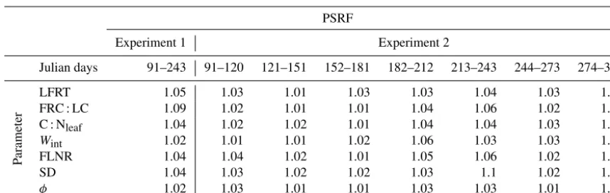
Table 2.Gelman–Rubin potential scale reduction factor (PSRF) of each Biome-BGC parameter selected for calibration andφ (nuisance parameter of likelihood function of Eq. 5) for Experiments 1 and 2. Information about the Biome-BGC parameters is given in Table 1. SD is the effective soil rooting depth.

PSRF

Experiment 1 Experiment 2

Julian days 91–243 91–120 121–151 152–181 182–212 213–243 244–273 274–304

P

arameter

LFRT 1.05 1.03 1.01 1.03 1.03 1.04 1.03 1.01

FRC : LC 1.09 1.02 1.01 1.01 1.04 1.06 1.02 1.01

C : Nleaf 1.04 1.02 1.02 1.01 1.04 1.04 1.03 1.03

Wint 1.02 1.01 1.01 1.02 1.06 1.03 1.03 1.01

FLNR 1.04 1.04 1.02 1.01 1.05 1.06 1.02 1.01

SD 1.04 1.03 1.02 1.02 1.03 1.1 1.02 1.02

φ 1.02 1.03 1.01 1.01 1.03 1.03 1.01 1.01

Biome-BGC reproduces the flux tower GPP. Both criteria provide a single measure of Biome-BGC efficiency in sim-ulating daily GPP over the selected period. The first criterion was the root mean square error (RMSE) between the simu-lated and flux tower GPP:

RMSE= v u u t 1

n n X

t=1

(zt−yt)2, (7)

where n is the number of daily flux tower GPP (zt) and

the simulated GPP (yt). RMSE has the unit of GPP. A low

value of RMSE indicates high accuracy. The second criterion was the Nash–Sutcliffe efficiency (NSE) (Nash and Sutcliffe, 1970):

NSE=1− Pn

t=1(zt−yt)2 Pn

t=1(zt−z)2

, (8)

wherez is the mean of the observations (flux tower GPP). NSE can range from−∞to 1. An NSE value close to 1 in-dicates high accuracy in the simulation of GPP. Following Dumont et al. (2014), we assumed that an NSE≥0.5 indi-cates adequate accuracy in the simulated GPP.

We evaluated the performance of Biome-BGC for the fol-lowing cases:

1. For Experiment 1, we obtained RMSE and NSE for the two periods: the calibration period of 5 months (April to August) and the validation period of 2 months (Septem-ber and Octo(Septem-ber). For each period, the calculations were made for 2.5 percentiles, 97.5 percentiles, and medi-ans. Note that the RMSE and NSE are typically eval-uated at the median of the posterior predictive distribu-tion; however, this does not evaluate the posterior un-certainty (Hamm et al., 2015a). Therefore, we also cal-culated the RMSE and NSE for the 2.5 and 97.5 per-centiles of the posterior GPP (y2.5andy97.5) against the same percentiles of flux tower GPP (z2.5andz97.5).

2. For Experiment 2, we obtained RMSE and NSE for the same two periods and percentiles as stated in point 1 (above), to make a direct comparison with the results of Experiment 1.

3. To show the performance of uncalibrated Biome-BGC, we obtained the daily simulated GPP with 95 % credible intervals at the prior distributions of six selected param-eters (Table 1). We sampled from these prior distribu-tions to obtain 50 000 parameter vectors. Biome-BGC was run at these parameter vectors to yield the prior pre-dictor of Biome-BGC simulated GPP (hereafter referred to as prior GPP). We calculated the RMSE and NSE for the same two periods and percentiles as stated in point 1, to make a direct comparison with Experiments 1 and 2.

4 Results

4.1 Convergence of the Markov chains

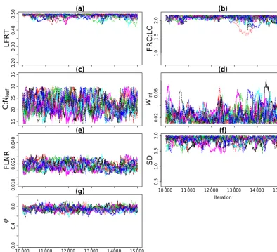
The value of the Gelman–Rubin PSRF was close to 1 for eachθj obtained in both experiments (Table 2). Figure 1a–f

show the trace plots of eachθj for Experiment 1. Visual

in-spection of the trace plots indicated that all 10 Markov chains were mixed properly with each other. For Experiment 2, we also observed the convergence of the Markov chains for each

θj in each month of the growing season (trace plots not

shown here). The visual and statistical diagnostics demon-strated that eachθj had explored its range and the obtained

samples from the converged chains were the samples from the posterior distribution.

Figure 1g shows the trace plot ofφ, accounting for the temporal correlation in the error residuals (Sect. 3.3.2), for Experiment 1. We observedφ6=0 and its value ranged from 0.56 to 0.93 with a mean at 0.75. The non-zero values ofφ

Ex-Figure 1.Trace plot of each calibrated Biome-BGC parameter andφ(nuisance parameter of likelihood function of Eq. 5) for Experiment 1 after the burn-in period of 10 000. Information about the Biome-BGC parameters is given in Table 1. SD is the effective soil rooting depth.

periment 2, non-zero values ofφwere also obtained in each month.

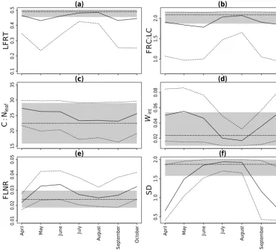
4.2 Posterior distribution of Biome-BGC parameters Figure 2 shows the temporal profile of median and 95 % cred-ible intervals of each θj over the growing season for

Ex-periment 2. For ExEx-periment 1, we obtained a single value for the median and 95 % credible intervals. For both ex-periments, we observed that the uncertainty in the posterior distribution of each θj was reduced compared to the prior

distribution, indicating that θ values were constrained by the flux tower GPP observations. These uncertainties were higher in Experiment 2 than in Experiment 1. The upper quantiles (97.5 %) of the posterior distributions of the pa-rameters LFRT, FRC : LC, and SD were found close to the maximum values of the corresponding prior distributions for both experiments. The uniform priors of these parameters (Table 1) possibly imposed an upper boundary in the poste-riors, which is called edge effect. Prior uniform distributions could be made wider in order to eliminate the edge effect.

However, we chose to keep these maximum values since the choices, given in Table 1, were based on the realistic ranges of LFRT, FRC : LC, and SD for Douglas fir at Speulderbos. For FRC : LC, previous work (Raj et al., 2014) on the study area found the maximum limit of FRC : LC was up to 6.85. However, we did not use the limit of 6.85 to make the uni-form distribution of FRC : LC wider in the present study. Raj et al. (2014) found that the increase of upper limit of the uniform distribution of FRC : LC from 2.16 to 6.85 led to the simulation with no development in LAI (leaf area index) and hence no production at the study site. The upper limit of FRC : LC at 2.16, however, fully supported the development of LAI at the study site. Therefore, we kept the upper limit of FRC : LC at 2.16 in the present study.

Figure 2. Median (solid lines) and 95 % credible intervals (dashed lines) of the posterior distributions of each calibrated Biome-BGC parameter obtained from Experiment 2 for each month during the growing season of 2009. The grey shade and dotted–dashed line represent median and 95 % credible intervals obtained for Experiment 1. The range of they axis represents the prior uncertainty in Biome-BGC parameters. Information about the Biome-BGC parameters is given in Table 1. SD is the effective soil rooting depth.

C : Nleaf and FLNR withr=0.95. This strong positive cor-relation is in line with the formulation of FLNR that shows direct proportionality with C : Nleaf (see Appendix A in Raj et al., 2014, for details). The parameters C : Nleafand FLNR showed similar negative, but weak (>−0.5), correlation with

Wint (r≈ −0.4). This can be explained by the fact that the simulated GPP is expected to vary inversely with Wint via soil water potential and stomatal regulation and directly with FLNR and C : Nleaf(see Sect. 5.1 for details of Biome-BGC internal routines). The parameter SD had similar positive, but weak (<0.5), correlation with FLNR and C : Nleaf(r≈0.4). This can be explained by the fact that the simulated GPP is expected to vary directly with SD (via soil water potential and stomatal regulation), and FLNR and C : Nleaf. Two pa-rameters of any other pair combinations did not show any notable correlation.

For Experiment 2, the uncertainties in LFRT, FRC : LC,

Wint, and SD were higher at the start and end of the growing

season compared to other months. The uncertainties in these parameters were lowest for calibration to GPP values of the peak of the growing season (July and August). The values of LFRT, FRC : LC, and SD increased during the peak of the growing season and became close to those obtained in Ex-periment 1 and then started decreasing. The opposite trend was observed forWint. The uncertainty in C : Nleaf for any month obtained in Experiment 2 was comparable and within the range of that obtained in Experiment 1. We did not find significant variation in the trend of FLNR obtained in Exper-iment 2 during the growing season; however, higher uncer-tainty in FLNR was observed compared to Experiment 1. 4.3 Evaluation of calibrated Biome-BGC for

Experiment 1

LFRT

1.6

1.8

2.0

FRC:LC

15

20

25

30

C:N

0.02

0.06

W

0.020

0.030

FLNR

0.42 0.46 0.50

1.4

1.6

1.8

2.0

1.6 1.8 2.0 15 20 25 30 0.02 0.06 0.020 0.030

SD

Figure 3.Correlation coefficient and scatterplot between the posterior distributions of each pair of calibrated Biome-BGC parameters ob-tained from Experiment 1. Information about the Biome-BGC parameters is given in Table 1. SD is the effective soil rooting depth.

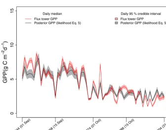
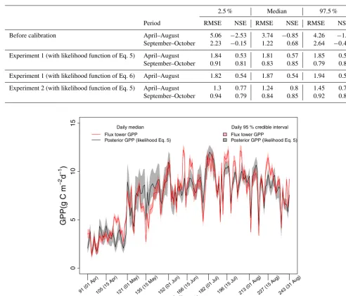
the validation period of September and October (Fig. 5). The daily posterior GPP values were summarized by the median and 95 % credible intervals. The temporal profiles of these medians and credible intervals were plotted against those of flux tower GPP. Evaluation of the Biome-BGC before and af-ter calibration (Experiment 1) based on the statistical criaf-teria (RMSE and NSE) is shown in Table 3. The periods for which these criteria were obtained are explained in Sect. 3.3.4.

Overall, daily posterior GPP was close to flux tower GPP during the calibration period (Fig. 4), although the separation between these two temporal profiles in April (Julian days 91 to 120) was large compared to other months (Julian days 121 to 242) in the growing season. For the validation period, pos-terior GPP closely followed the flux tower GPP (Fig. 5).

The posterior GPP was improved compared with the prior GPP, as indicated by the drop of RMSE for the median as well as the 2.5 and 97.5 percentiles for both calibration and validation periods (Table 3). The NSE criterion was also im-proved after calibration (NSE>0.5), whereas before calibra-tion, the value of NSE was negative. The enhancement in NSE and the drop of RMSE give statistical evidence of the improvement in the daily prior GPP after calibration.

We also evaluated the performance of calibrated Biome-BGC using the likelihood function without the temporal cor-relation in the residuals (Eq. 6). The obtained daily

me-dians of posterior GPP for the calibration period (April– August) are shown in Fig. 4. For daily medians as well as 2.5 and 97.5 percentiles, RMSE and NSE criteria are shown in Table 3. We found that both likelihood functions Eqs. (5) and (6) led to similar temporal profiles of the posterior GPP and similar values of RMSE and NSE criteria.

4.4 Posterior GPP for Experiment 2

com-0

5

10

15

GPP

(g C

m

−

2

d

−

1

)

91 (01 Apr)105 (15 Apr)121 (01 May

)

135 ( 15 M

ay)

152 ( 01 Ju

n)

166 ( 15 Ju

n)

182 ( 01 Ju

l)

196 ( 15 Ju

l)

213 ( 01 A

ug)

227 ( 15 A

ug)

243 ( 31 A

ug)

Julian day

Flux tower GPP

Posterior GPP (likelihood Eq. 5) Posterior GPP (likelihood Eq. 6)

Daily 95 % credible interval Flux tower GPP

Posterior GPP (likelihood Eq. 5)

Figure 4.Temporal profile of daily posterior GPP, obtained from Experiment 1, and daily flux tower GPP for the calibration period of 5 months (April to August, Julian days 91 to 243). Daily medians and 95 % credible intervals of posterior GPP, obtained using likelihood function of Eq. (5), are represented by the solid black line and grey shade, respectively. Daily medians of posterior GPP, obtained using likelihood function of Eq. (6), are represented by the dotted black line. Daily medians and 95 % credible intervals of flux tower GPP values are represented by the red line and light red shade, respectively.

0

5

10

15

GPP

(g C

m

−

2

d

−

1

)

244 (01 Sep) 258 (15 Sep) 274 (01 Oct) 288 (15 Oct) 304 (31 Oct)

Julian day

Daily median Flux tower GPP

Posterior GPP (likelihood Eq. 5)

Daily 95 % credible interval Flux tower GPP

Posterior GPP (likelihood Eq. 5)

Table 3.Root mean square error (RMSE) and Nash–Sutcliffe efficiency (NSE) between the prior (before calibration)/posterior GPP and flux tower GPP for different experiments (see Sect. 3.3.4) and likelihoods (see Sect. 3.3.2).

2.5 % Median 97.5 %

Period RMSE NSE RMSE NSE RMSE NSE

Before calibration April–August 5.06 −2.53 3.74 −0.85 4.26 −1.3

September–October 2.23 −0.15 1.22 0.68 2.64 −0.42

Experiment 1 (with likelihood function of Eq. 5) April–August 1.84 0.53 1.81 0.57 1.85 0.57 September–October 0.91 0.81 0.83 0.85 0.79 0.87

Experiment 1 (with likelihood function of Eq. 6) April–August 1.82 0.54 1.87 0.54 1.94 0.52

Experiment 2 (with likelihood function of Eq. 5) April–August 1.3 0.77 1.24 0.8 1.45 0.73 September–October 0.94 0.79 0.84 0.85 0.92 0.83

0

5

10

15

GPP

(g C

m

−

2

d

−

1

)

91 (01 Apr)105 (15 Apr)121 (01 M ay)

135 ( 15 M

ay)

152 ( 01 Ju

n)

166 ( 15 Ju

n)

182 ( 01 Ju

l)

196 ( 15 Ju

l)

213 ( 01 A

ug)

227 ( 15 A

ug)

243 ( 31 A

ug)

Julian day

Flux tower GPP

Posterior GPP (likelihood Eq. 5)

Daily 95 % credible interval Flux tower GPP

Posterior GPP (likelihood Eq. 5)

Figure 6.Temporal profile of daily posterior GPP, obtained from Experiment 2, and daily flux tower GPP for 5 months (April to August, Julian days 91 to 243). Other details are as for Fig. 4.

pared to that obtained from Experiment 1 but at the expense of a higher degree of freedom.

5 Discussion

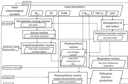
5.1 Simulation of GPP using Biome-BGC

To explain our results, we identified the processes within Biome-BGC that are controlled by the six calibrated param-eters and relate to the simulation of GPP (Fig. 7). These pro-cesses are implemented by different routines. The routines, however, are controlled not only by these six parameters but

also generate intermediate outputs, as shown in Fig. 7. We only highlight those routines that were relevant to the simu-lation of GPP. We refer the reader to Thornton (2010) for a detailed explanation of the routines.

LFRT Input

meteorological

variables Wint SD FLNR C:Nleaf FRC:LC

Evapotranspiration routine Photosynthesis routine

Radiation transfer routine Development of

leaf carbon

Photosynthesis routine

Farquhar photosynthesis model

Temperature

Daily gross primary production Input parameters

Respiration routine

Temperature, day length

Day length

Precipitation routing routine

Soil water

Soil psi routine

Soil water potential

Leaf-scale conductance to water vapour

Carbon assimilation

Day leaf maintenance respiration Leaf area index

Leaf nitrogen content Leaf-scale conductance to

CO2

Radiation

Temperature, vapour pressure deficit Precipitation

Figure 7.The Biome-BGC internal routines that simulate GPP, controlled by the meteorological data and the six calibrated parameters. Rectangular boxes represent the Biome-BGC routines and the parallelograms represent the input and output of the routine. Information about the Biome-BGC parameters is given in Table 1.

routine. Leaf C relates to the loss of leaf biomass, which is expressed as the parameter LFRT. The parameter FRC : LC is also responsible for the development of leaf C and then LAI. In the precipitation routine,Wint, together with LAI, deter-mine the amount of precipitation intercepted by the canopy, which in turns controls the amount of water that reaches the soil. The soil matric potential (psi) routine calculates the vol-umetric water content in the soil as the ratio of soil water to SD. Thereafter, soil water potential is derived as a function of volumetric water content. The soil water potential acts as a multiplier in the evapotranspiration routine to simulate stom-atal closure and the leaf-scale conductance to water vapour per unit leaf area.

The photosynthesis routine converts the conductance to water vapour to the conductance for CO2, which measures the rate of passage of CO2into the leaf stomata. The param-eter C : Nleaftogether with LAI determines the leaf nitrogen content from the carbon pool in the photosynthesis routine and the day leaf maintenance respiration per unit leaf area in the respiration routine. The leaf-scale conductance to CO2, leaf nitrogen content, day leaf maintenance respiration, and the parameter FLNR are further used in the Farquhar model, implemented in the photosynthesis routine, to simulate the carboxylation capacity (Vcmax) and thus the carbon assimi-lation. The assimilated carbon is then added to the day leaf

maintenance respiration and then multiplied by the LAI and day length to simulate the daily GPP. The respiration routine also calculates the maintenance respiration of roots and stems (not shown in Fig. 7) together with leaves. The respiration terms are summed and then subtracted from GPP to obtain available carbon for allocation, which further updates leaf C. Finally, Fig. 7 indicates which meteorological variables are used in a given routine, although we have not described their specific role.

We presented the link between six calibrated parameters and the Biome-BGC internal routines so that we could ex-plain our results considering the development of the state variables, principally such as LAI andVcmax. LAI andVcmax exhibit a seasonal cycle and affect the seasonality of simu-lated GPP. This is explored further in Sect. 5.2.

5.2 Biome-BGC calibration

The posterior GPP closely followed the flux tower GPP even for those months (September and October) which were not included in the calibration (Fig. 5), although this was not perfect as shown by the fact that φ6=0. If the simulator would properly capture the temporal development of GPP, we would expect that φ=0, even after allowing for some uncertainty in the prediction. We deliberately assumedφ=0 in the likelihood function (Eq. 6) to check if this assumption has any effect on the posterior GPP. We, however, found that both choices,φ6=0 andφ=0, led to similar posterior GPP (Sect. 4.3). This comparison indicated that an improvement in temporal development of GPP after calibration might not be achieved, at least for the Biome-BGC simulator, with ei-ther the assumption of presence or absence of temporal cor-relation in the residuals. The representation of dynamic pro-cesses within the simulator responsible for GPP should be, therefore, given more attention in order to improve the tem-poral development of GPP. This is what we showed in Ex-periment 2.

Experiment 1 showed that Biome-BGC was able to repro-duce closely the flux tower GPP. Further, the Bayesian cal-ibration allowed daily posterior GPP simulation as well as quantification of the associated uncertainty (Figs. 4 and 5). The edge effect in the posterior distributions of the param-eters LFRT, FRC : LC, and SD (Sect. 4.2) could be seen as the deficiency of the calibration. A drop in RMSE and en-hancement in NSE coefficient (Table 3) before and after cal-ibration, however, indicated the efficiency of the calibration. Furthermore, the apparent overprediction of daily posterior GPP, compared to flux tower GPP, for the month of April raised questions (a) on the reliability of posterior GPP for those months that were not included in this study, and (b) of whether the seasonal cycle of all of the state variables was simulated realistically. These questions led us to estimate the posterior distributions of parameters for different months representing the phenological cycle in Experiment 2.

Consider Experiment 2. Note that Biome-BGC actually simulated daily posterior GPP for a whole year with the pos-terior distributions of the parameters of each month. We se-lected only the daily posterior GPP of that month to which the posterior distributions belong and we discarded the other 11 months of simulations. The temporal profile in Fig. 6 con-tains the combinations of daily posterior GPP of each month in the growing season (Sect. 3.3.3 and 4.4). Thus, the tem-poral profile of daily posterior GPP in Experiment 2 was obtained by mixing several independently simulated time se-ries. The resulting time series has discontinuities in state vari-ables, and thus the update of simulator memory (Sect. 5.1) between the months is ignored. This time series can, how-ever, help to analyse the simulator behaviour for the tem-poral variation in the input parameters. Alternatively, one could think of updating the simulator state at the end of a month. This would then be the starting state for the run of the next month with changed parameters. This approach, how-ever, can not be implemented in the original configuration of

Biome-BGC, because a single forward run of Biome-BGC simulates output for at least 1 year and accepts only con-stant input parameters. These parameters can not be changed across months in a single forward run. This would require changing the Biome-BGC code. Such a modification was, however, not desired because model deficiency of Biome-BGC could still be investigated through the temporal vari-ation in the input parameters across the season using the ap-proach proposed in Experiment 2. Biome-BGC was there-fore calibrated against the data of each month separately, as if information on GPP for the other months was absent. If the obtained variations in the input parameters improve the seasonality in simulated GPP, this indicates that the default linkage of the constant parameters with the state variables, that change during the season, in the simulator may require improvement in future studies.

We observed an improvement (Fig. 6), particularly in the month of April, in the daily posterior GPP compared to Ex-periment 1 (Fig. 4). This improvement was also clear in Ta-ble 3 which shows an increase in the NSE and decrease in the RMSE for Experiment 2 compared to Experiment 1. More interestingly, Experiment 2 showed variation in the six cali-brated parameters depending on the month Biome-BGC was calibrated to (Fig. 2), particularlyWint, SD , FRC : LC, and LFRT. These variations were also in line with the seasonal variation in GPP. For example, maintaining the high GPP rates during the peak of the growing season (July and Au-gust), required lowerWintand higher SD, both increasing the soil water availability through the precipitation routing rou-tine in Fig. 7. During the start of growing season (April), higherWint and lower SD maintained low GPP rates. This suggests that either the soil water reservoir or the feedback mechanism between soil moisture and stomatal conductiv-ity via the soil water potential was responsible for the un-derestimation and overestimation of simulated GPP in Ex-periment 1. The parameters FRC : LC and LFRT were also higher when calibrated to summer months. Both parameters affect GPP through LAI. The variation in FLNR and C : Nleaf, which together determine Vcmax, also changed month by month (Fig. 7). The results of Experiment 2 indicated that Biome-BGC may be too rigid to simulate the seasonality of the state variables (LAI andVcmax), at least in evergreen coniferous forests, without the temporal variation in the in-put parameters and thus highlighted the model deficiency of Biome-BGC. To our knowledge, this aspect has not been dis-cussed in earlier work on the calibration of Biome-BGC (Yan et al., 2014; Ueyama et al., 2010; Maselli et al., 2008).

the input parameters, related to photosynthetic capacity, of Biome-BGC in a Bayesian framework. We observed that the temporal dynamics of the state variables (LAI andVcmax) and the soil water mechanism within Biome-BGC, and thus pho-tosynthesis, are not sufficiently expressed by the constant in-put parameters. These state variables also control photosyn-thesis simulations in other process-based simulators, such as SCOPE (van der Tol et al., 2009), and are governed by the constant input parameters that may not be adequate based on our findings. Our study, therefore, reinforces a message that the reconsideration of temporal dynamics of state variables within the simulator, possibly through the temporal varia-tion in the parameters, should receive further attenvaria-tion to the modelling communities focusing on simulating the for-est carbon cycle.

The major metrics of the carbon cycle include GPP, ecosystem respiration (Reco), and NEE. In this study, we lim-ited the calibration to partitioned flux tower GPP. A limi-tation of this approach is that the output of process-based simulators is calibrated against the output of another model, notably the flux partitioning model. The latter is not a pro-cess model but a semi-empirical model calibrated to 10-day blocks of data (Sect. 3.1.2). Although this approach has been used in many other studies that validate the output of process-based simulators (Zhou et al., 2016; Collalti et al., 2016; Liu et al., 2014; Yuan et al., 2014), it would also be possible to calibrate Biome-BGC using this approach. More importantly, a calibration to NEE data (i.e. difference between GPP and

Reco) alone does not guarantee that GPP andRecoterms are well calibrated. Other studies (Kuppel et al., 2012; Fox et al., 2009) that used NEE data to calibrate process-based simula-tors such as DALEC (Data Assimilation Linked Ecosystem Carbon) and ORCHIDEE, therefore, were more successful in achieving the accuracy of this simulated difference compared to GPP and Reco. Tang and Zhuang (2009) showed the im-provement (by the drop of RMSE) in simulated GPP andReco by the process-based simulator TEM (Terrestrial Ecosystem Model) when both GPP andRecodata were used in calibra-tion as compared to using NEE data alone. In our study, we decided to test the calibration algorithm for GPP first. This approach can be extended to includeRecodata together with NEE data in order to ensure the accuracy of all simulated metrics of carbon cycle. Then the parameters, which may in-fluence the simulatedReco, need to be identified and should be included in the calibration.

We performed our calibration based on six parameters (LFRT, FRC : LC, C : Nleaf,Wint, FLNR, and SD), whereas Biome-BGC has 35 parameters in total. A calibration based on 35 parameters was not feasible computationally, so, in line with other authors (e.g. Minunno et al., 2013), we chose a subset of the parameters. We defend our choice of parameters based on our previous experimental results, which showed that annual total GPP was most sensitive to these parameters (Raj et al., 2014) at Speulderbos. Nevertheless, GPP may be sensitive to other parameters at finer spatial scales.

Compu-tational developments and the flexibility of the DREAM al-gorithm may allow more parameters to be calibrated. This could lead to a more comprehensive calibration to multiple outputs in the near future.

6 Conclusions

This study presented a Bayesian calibration framework for the simulator Biome-BGC. We illustrated the framework at the Speulderbos Forest site in the Netherlands. Use of the framework led to the following conclusions:

1. The Bayesian framework allowed quantification of un-certainty in both the estimated parameters and the pos-terior (predictive) GPP, through the pospos-terior (predic-tive) distribution. The uncertainty is important in the sense that it helps to determine how much confidence can be placed in the results of forest carbon-related stud-ies based on GPP. A calibration based on optimization of Biome-BGC parameters, as done in earlier studies, can not capture the associated uncertainty in the simu-lated GPP.

2. We modelled the temporal correlation in the residuals through the nuisance parameter, φ, in the likelihood function. We concluded that Biome-BGC did not prop-erly simulate the temporal development of GPP, nei-ther by assuming temporal correlation in the residuals (φ6=0) nor by ignoring this (φ=0) and the dynamical processes within the Biome-BGC became more promi-nent. Hence, calibration gave greater insight into the simulator. Other future studies on the calibration of sim-ilar process-based simulators may also ignore φ, but they should consider carefully the dynamic processes within the simulators to achieve improved calibration results.

3. We used the calibration results to gain further insights into the functioning (dynamic processes) of Biome-BGC through analysis of the monthly variation in pos-terior parameter distributions. Our study revealed the model deficiency of Biome-BGC for using constant pa-rameters to simulate seasonality of state variables and thus the seasonality in daily GPP. The seasonality was captured more precisely by using monthly variation in the Biome-BGC parameters. In future, such model de-ficiency should receive attention from the Biome-BGC modelling communities. Nevertheless, our findings also suggest that the other modelling communities that use the similar process-based simulators may also consider to improve such model deficiency.

implementations. It shows promise for biogeochemi-cal and other environmental simulation applications. Specifically, future research could calibrate more pa-rameters.

Code and data availability. We provide a MatLab script and in-put data as supplementary material to support the implementation of Bayesian calibration of the Biome-BGC simulator. The Mat-Lab script uses the functionality of the DREAM toolbox, which can be obtained, on request, from its developer, Jasper A. Vrugt, University of California, Davis, USA (Vrugt, 2016). The source code of the Biome-BGC simulator can be downloaded from http: //www.ntsg.umt.edu/project/biome-bgc. Markov chains in DREAM are run in parallel using multiple cores of the computer processors. DREAM consumes a large amount of memory (RAM). The exper-iment shown in this paper was performed on Windows Server 2012 Dell Precision 7910 with a 12-core Xeon processor and 128 GB of RAM.

Additional information on code and data can be found in Raj (2016).

Information about the Supplement

The description of each file in the supplementary material is given below:

1. MatLab scripts:

(a) DREAM_setup.m: This scripts defines the ba-sic settings of DREAM, which were used in our experiment. The script is self-explanatory. This script calls the MatLab function (“BIOME-BGCrunScript.m”) to run Biome-BGC simulator. (b) BIOME-BGCrunScript.m: This scripts defines the

function to run Biome-BGC (by calling point-bgc.exe) simulator with the parameter value ob-tained in each iteration of DREAM and the daily simulated GPP is returned. We do not provide “pointbgc.exe”. This can be obtained by compiling Biome-BGC source code.

2. Input data files used to run Biome-BGC in our exper-iment (for details, see the Biome-BGC user guide that comes with the source code of Biome-BGC):

(a) enf_speuld_Main.ini: This is the input initialization file. It provides general information about the sim-ulation such as site characteristics data, the name of all required input files and output files, and lists of output variables to be stored.

(b) Meanpm.epc: This is the input parameters file that contains the mean value of each parameter. (c) Speuld2009.mtc41: This file contains daily input

meteorological variables of 2009 at the Speulder-bos site in the Netherlands.

3. Input flux tower GPP (for calibration and comparison with posterior simulated GPP):

(a) Percentiles_FluxTower_GPP_JD_91_304.xlsx: This Excel file contains the mean and percentiles of daily GPP (for the growing season of 2009) partitioned from flux tower measurements of net ecosystem exchange at the Speulderbos Forest site in the Netherlands. Daily mean values were used in calibration and percentile values were used to compare with posterior simulated GPP.

(b) TowerGPP.txt: This file contains the subset (from Julian days 91 to 243 in Experiment 1; see Sec-tion 3.3.3) of daily mean of flux tower GPP. This file is called in “DREAM_setup.m”. For Experiment 2, different subsets of flux tower GPP can be easily obtained from the file “Per-centiles_FluxTower_GPP_JD_91_304.xlsx”.

The Supplement related to this article is available online at https://doi.org/10.5194/gmd-11-83-2018-supplement.

Competing interests. The authors declare that they have no conflict of interest.

Acknowledgements. Biome-BGC version 4.2 was provided by

Peter Thornton at the National Center for Atmospheric Research (NCAR) and by the Numerical Terradynamic Simulation Group (NTSG) at the University of Montana, USA. NCAR is sponsored by the National Science Foundation. The authors thankfully acknowledge the support of the Erasmus Mundus mobility grant and the University of Twente for funding this research. The authors acknowledge Jasper A. Vrugt, from the University of California, Davis, USA for providing the DREAM toolbox.

Edited by: Philippe Peylin

Reviewed by: Thomas Wutzler and one anonymous referee

References

Bastin, L., Cornford, D., Jones, R., Heuvelink, G. B. M., Pebesma, E., Stasch, C., Nativi, S., Mazzetti, P., and Williams, M.: Man-aging uncertainty in integrated environmental modelling: The UncertWeb framework, Environ. Model. Softw., 39, 116–134, https://doi.org/10.1016/j.envsoft.2012.02.008, 2013.

Churkina, G. and Running, S. W.: Contrasting climatic controls on the estimated productivity of global terrestrial biomes, Ecosys-tems, 1, 206–215, 1998.

Collalti, A., Marconi, S., Ibrom, A., Trotta, C., Anav, A., D’Andrea, E., Matteucci, G., Montagnani, L., Gielen, B., Mammarella, I., Grünwald, T., Knohl, A., Berninger, F., Zhao, Y., Valen-tini, R., and SanValen-tini, M.: Validation of 3D-CMCC Forest Ecosystem Model (v.5.1) against eddy covariance data for 10 European forest sites, Geosci. Model Dev., 9, 479–504, https://doi.org/10.5194/gmd-9-479-2016, 2016.

Constable, J. V. H. and Friend, A. L.: Suitability of process-based tree growth models for addressing tree response to climate change, Environ. Pollut., 110, 47–59, 2000.

Dumont, B., Leemans, V., Mansouri, M., Bodson, B., Destain, J. P., and Destain, M. F.: Parameter identification of the STICS crop model, using an accelerated formal MCMC approach, Environ. Model. Softw., 52, 121–135, 2014.

Farquhar, G. D., von Caemmerer, S., and Berry, J. A.: A biochem-ical model of photosynthetic CO₂assimilation in leaves of C₃ species, Planta, 149, 78–90, 1980.

Fox, A., Williams, M., Richardson, A. D., Cameron, D., Gove, J. H., Quaife, T., Ricciuto, D., Reichstein, M., Tomelleri, E., Trudinger, C. M., and Van Wijk, M. T.: The REFLEX project: Comparing different algorithms and implementations for the inversion of a terrestrial ecosystem model against eddy covariance data, Agr. Forest Meteorol., 149, 1597–1615, https://doi.org/10.1016/j.agrformet.2009.05.002, 2009.

Gelfand, A. E. and Smith, A. F. M.: Sampling-based approaches to calculating marginal densities, J. Am. Stat. Assoc., 85, 398–409, 1990.

Gelman, A. and Rubin, D. B.: Inference from iterative simulation using multiple sequences, Stat. Sci., 7, 457–511, 1992.

Gelman, A., Carlin, J. B., Stern, H. S., Dunson, D. B., Vehtari, A., and Rubin, D. B.: Bayesian Data Analysis, CRC press, Boca Ra-ton, 639 pp., 2013.

Gilmanov, T. G., Verma, S. B., Sims, P. L., Meyers, T. P., Bradford, J. A., Burba, G. G., and Suyker, A. E.: Gross primary production and light response parameters of four Southern Plains ecosystems estimated using long-term CO2 -flux tower measurements, Global Biogeochem. Cy., 17, 1071, https://doi.org/10.1029/2002GB002023, 2003.

Hamm, N. A. S., Finley, A. O., Schaap, M., and Stein, A.: A spatially varying coefficient model for mapping air qual-ity at the European scale, Atmos. Environ., 102, 393–405, https://doi.org/10.1016/j.atmosenv.2014.11.043, 2015a. Hamm, N. A. S., Soares Magalhães, R. J., and Clements, A.

C. A.: Earth observation, spatial data quality and neglected tropical disesases, PLOS Neglect. Trop. D, 9, e0004164, https://doi.org/10.1371/journal.pntd.0004164, 2015b.

Hartig, F., Dyke, J., Hickler, T., Higgins, S. I., O’Hara, R. B., Scheiter, S., and Huth, A.: Connecting dynamic vegetation mod-els to data – an inverse perspective, J. Biogeogr., 39, 2240–2252, 2012.

Hastings, W. K.: Monte Carlo sampling methods using Markov chains and their applications, Biometrika, 57, 97–109, 1970. He, H., Liu, M., Xiao, X., Ren, X., Zhang, L., Sun, X., Yang, Y., Li,

Y., Zhao, L., Shi, P., Du, M., Ma, Y., Ma, M., Zhang, Y., and Yu, G.: Large-scale estimation and uncertainty analysis of gross

pri-mary production in Tibetan alpine grasslands, J. Geophys. Res.-Biogeo., 119, 466–486, 2014.

Kennedy, M. C. and O’Hagan, A.: Bayesian calibration of computer models, J. R. Stat. Soc. B, 63, 425–464, https://doi.org/10.1111/1467-9868.00294, 2001.

Kuppel, S., Peylin, P., Chevallier, F., Bacour, C., Maignan, F., and Richardson, A. D.: Constraining a global ecosystem model with multi-site eddy-covariance data, Biogeosciences, 9, 3757–3776, https://doi.org/10.5194/bg-9-3757-2012, 2012.

Liu, D., Cai, W., Xia, J., Dong, W., Zhou, G., Chen, Y., Zhang, H., and Yuan, W.: Global validation of a process-based model on vegetation gross primary production us-ing eddy covariance observations, PLOS ONE, 9, e110407, doi:10.1371/journal.pone.0110407, 2014.

Mäkelä, A., Landsberg, J., Ek, A. R., Burk, T. E., Ter-Mikaelian, M., Ägren, G. I., Oliver, C. D., and Puttonen, P.: Process-based models for forest ecosystem management: current state of the art and challenges for practical implementation, Tree Physiol., 20, 289–298, 2000.

Maselli, F., Chiesi, M., Fibbi, L., and Moriondo, M.: Integration of remote sensing and ecosystem modelling techniques to estimate forest net carbon uptake, Int. J. Remote Sens., 29, 2437–2443, 2008.

McNaughton, K. and Jarvis, P.: Predicting effects of vegetation changes on transpiration and evaporation, Water deficits plant growth, 7, 1–47, 1983.

Metropolis, N., Rosenbluth, A. W., Rosenbluth, M. N., Teller, A. H., and Teller, E.: Equation of state calculations by fast computing machines, The J. Chem. Phys., 21, 1087–1092, 1953.

Minunno, F., van Oijen, M., Cameron, D. R., and Pereira, J. S.: Selecting parameters for Bayesian calibration of a process-based model: A methodology based on canonical correlation analysis, SIAM J. Uncertainty Quantification, 1, 370–385, 2013. Mitchell, S., Beven, K., Freer, J., and Law, B.: Processes

influ-encing model-data mismatch in drought-stressed, fire-disturbed eddy flux sites, J. Geophys. Res.-Biogeo., 116, G02008, https://doi.org/10.1029/2009JG001146, 2011.

Mo, X., Chen, J. M., Ju, W., and Black, T. A.: Optimization of ecosystem model parameters through assimilating eddy covari-ance flux data with an ensemble Kalman filter, Ecol. Model., 217, 157–173, https://doi.org/10.1016/j.ecolmodel.2008.06.021, 2008.

Monteith, J. L. and Unsworth, M. H.: Principles of Environmen-tal Physics, Edward Arnold, Sevenoaks, UK, 2nd Edn., 291 pp., 1990.

Monteith, J. L. and Unsworth, M. H.: Principles of Environmental Physics, Academic Press, Burlington, Massachusetts, 3rd Edn., 440 pp., 2008.

Nash, J. E. and Sutcliffe, J. V.: River flow forecasting through con-ceptual models part I – A discussion of principles, J. Hydrol., 10, 282–290, 1970.

Raj, R.: Bayesian integration of flux tower data into process-based simulator for quantifying uncertainty in simulated output, DANS, https://doi.org/10.17026/dans-zc7-7549, 2016.

Raj, R., Hamm, N. A. S., van der Tol, C., and Stein, A.: Variance-based sensitivity analysis of BIOME-BGC for gross and net pri-mary production, Ecol. Model., 292, 26–36, 2014.

ecosys-tem exchange measurements, Biogeosciences, 13, 1409–1422, https://doi.org/10.5194/bg-13-1409-2016, 2016.

Reinds, G. J., van Oijen, M., Heuvelink, G. B. M., and Kros, H.: Bayesian calibration of the VSD soil acidification model us-ing European forest monitorus-ing data, Geoderma, 146, 475–488, 2008.

Running, S. W.: Testing Forest-BGC ecosystem process simulations across a climatic gradient in Oregon, Ecol. Appl., 4, 238–247, 1994.

Running, S. W. and Hunt, E. R.: Generalization of a forest ecosys-tem process model for other biomes, BIOME-BGC, and an ap-plication for global-scale models, in: Scaling physiological pro-cesses: Leaf to globe, edited by: Ehleringer, J. R. and Field, C. B., Academic Press, Inc., New York, 141–158, 1993.

Starrfelt, J. and Kaste, O.: Bayesian uncertainty assessment of a semi-distributed integrated catchment model of phosphorus transport, Environ. Sci.-Proc. Imp., 16, 1578–1587, 2014. Steingrover, E. G. and Jans, W. W. P.: Physiology of forest-grown

Douglas fir trees: Effect of air pollution and drought, Tech. Rep. 94/3, IBN DLO, Institute for Forestry and Nature Research, Wa-geningen, the Netherlands, 1994.

Su, Z., Timmermans, W. J., van der Tol, C., Dost, R., Bianchi, R., Gómez, J. A., House, A., Hajnsek, I., Menenti, M., Magliulo, V., Esposito, M., Haarbrink, R., Bosveld, F., Rothe, R., Baltink, H. K., Vekerdy, Z., Sobrino, J. A., Timmermans, J., van Laake, P., Salama, S., van der Kwast, H., Claassen, E., Stolk, A., Jia, L., Moors, E., Hartogensis, O., and Gillespie, A.: EAGLE 2006 – Multi-purpose, multi-angle and multi-sensor in-situ and airborne campaigns over grassland and forest, Hydrol. Earth Syst. Sci., 13, 833–845, https://doi.org/10.5194/hess-13-833-2009, 2009. Svensson, M., Jansson, P.-E., Gustafsson, D., Kleja, D. B., Langvall,

O., and Lindroth, A.: Bayesian calibration of a model describing carbon, water and heat fluxes for a Swedish boreal forest stand, Ecol. Model., 213, 331–344, 2008.

Tang, J. and Zhuang, Q.: A global sensitivity analysis and Bayesian inference framework for improving the parame-ter estimation and prediction of a process-based Terrestrial Ecosystem Model, J. Geophys. Res.-Atmos., 114, D15303, https://doi.org/10.1029/2009JD011724, 2009.

Thornton, P. E.: Description of a numerical simulation model for predicting the dynamics of energy, water, carbon, and nitrogen in a terrestrial ecosystem, PhD thesis, University of Montana, Missoula, 1998.

Thornton, P. E.: Biome-BGC version 4.2: Theoretical Framework of Biome-BGC, Technical Documentation, 2010.

Thornton, P. E. and Running, S. W.: User’s guide for Biome-BGC, Version 4.1.2, available at: http://www.ntsg.umt.edu/sites/ntsg. umt.edu/files/project/biome-bgc/bgc_users_guide_412.PDF, 2002.

Thornton, P. E., Law, B. E., Gholz, H. L., Clark, K. L., Falge, E., Ellsworth, D. S., Goldstein, A. H., Monson, R. K., Hollinger, D., Falk, M., Chen, J., and Sparks, J. P.: Modeling and measuring the effects of disturbance history and climate on carbon and water budgets in evergreen needleleaf forests, Agr. Forest Meteorol., 113, 185–222, 2002.

Ueyama, M., Ichii, K., Hirata, R., Takagi, K., Asanuma, J., Machimura, T., Nakai, Y., Ohta, T., Saigusa, N., Takahashi, Y., and Hirano, T.: Simulating carbon and water cycles of larch forests in East Asia by the BIOME-BGC model with AsiaFlux

data, Biogeosciences, 7, 959–977, https://doi.org/10.5194/bg-7-959-2010, 2010.

van der Tol, C., Verhoef, W., Timmermans, J., Verhoef, A., and Su, Z.: An integrated model of soil-canopy spectral radiances, photo-synthesis, fluorescence, temperature and energy balance, Biogeo-sciences, 6, 3109-3129, https://doi.org/10.5194/bg-6-3109-2009, 2009.

van Oijen, M., Rougier, J., and Smith, R.: Bayesian calibration of process-based forest models: bridging the gap between models and data, Tree Physiol., 25, 915–927, 2005.

van Oijen, M., Cameron, D. R., Butterbach-Bahl, K., Farahbakhs-hazad, N., Jansson, P. E., Kiese, R., Rahn, K. H., Werner, C., and Yeluripati, J. B.: A Bayesian framework for model calibration, comparison and analysis: Application to four models for the bio-geochemistry of a Norway spruce forest, Agr. Forest Meteorol., 151, 1609–1621, 2011.

van Oijen, M., Reyer, C., Bohn, F. J., Cameron, D. R., Deckmyn, G., Flechsig, M., Härkönen, S., Hartig, F., Huth, A., Kiviste, A., Lasch, P., Mäkelä, A., Mette, T., Minunno, F., and Rammer, W.: Bayesian calibration, comparison and averaging of six forest models, using data from Scots pine stands across Europe, Forest Ecol. Manag., 289, 255–268, 2013.

van Wijk, M. T., Dekker, S. C., Bouten, W., Kohsiek, W., and Mohren, G. M. J.: Simulation of carbon and water budgets of a Douglas-fir forest, Forest Ecol. Manag., 145, 229–241, 2001. Verstegen, J. A., Karssenberg, D., van der Hilst, F., and Faaij,

A. P.: Identifying a land use change cellular automaton by Bayesian data assimilation, Environ. Model. Softw., 53, 121– 136, https://doi.org/10.1016/j.envsoft.2013.11.009, 2014. Vrugt, J. A.: Markov chain Monte Carlo simulation using the

DREAM software package: Theory, concepts, and MATLAB im-plementation, Environ. Model. Softw., 75, 273–316, 2016. Vrugt, J. A., ter Braak, C. J. F., Clark, M. P., Hyman, J. M.,

and Robinson, B. A.: Treatment of input uncertainty in hy-drologic modeling: Doing hydrology backward with Markov chain Monte Carlo simulation, Water Resour. Res., 44, W00B09, doi:10.1029/2007WR006720, 2008.

Vrugt, J. A., ter Braak, C. J. F., Diks, C. G. H., Robinson, B. A., Hy-man, J. M., and Higdon, D.: Accelerating Markov chain Monte Carlo simulation by differential evolution with self-adaptive ran-domized subspace sampling, Int. J. Nonlin. Sci. Num., 10, 273– 290, 2009.

White, M., Thornton, P., Running, S., and Nemani, R.: Parameter-ization and sensitivity snalysis of the BIOME-BGC terrestrial ecosystem model: Net primary production controls, Earth Inter-act., 4, 1–85, 2000.

Williams, M., Richardson, A. D., Reichstein, M., Stoy, P. C., Peylin, P., Verbeeck, H., Carvalhais, N., Jung, M., Hollinger, D. Y., Kattge, J., Leuning, R., Luo, Y., Tomelleri, E., Trudinger, C. M., and Wang, Y.-P.: Improving land surface models with FLUXNET data, Biogeosciences, 6, 1341–1359, https://doi.org/10.5194/bg-6-1341-2009, 2009.

Xenakis, G., Ray, D., and Mencuccini, M.: Sensitivity and uncer-tainty analysis from a coupled 3-PG and soil organic matter de-composition model, Ecol. Model., 219, 1–16, 2008.

Yuan, W., Cai, W., Xia, J., Chen, J., Liu, S., Dong, W., Merbold, L., Law, B., Arain, A., Beringer, J., Bernhofer, C., Black, A., Blanken, P. D., Cescatti, A., Chen, Y., Francois, L., Gianelle, D., Janssens, I. A., Jung, M., Kato, T., Kiely, G., Liu, D., Marcolla, B., Montagnani, L., Raschi, A., Roupsard, O., Varlagin, A., and Wohlfahrt, G.: Global comparison of light use efficiency mod-els for simulating terrestrial vegetation gross primary production based on the LaThuile database, Agr. Forest Meteorol., 192–193, 108–120, 2014.