Estimation of greenhouse gas emissions from spontaneous combustion/fire of coal in opencast mines – Indian context

(1)

Estimation of Greenhouse Gases Emissions from Spontaneous Combustion/Fire of Coal in Opencast Mines – Indian Context

*N. K. Mohalik1_{, E. Lester}2_{, I.S. Lowndes}3_{and V. K. Singh}4

1_{Senior Scientist,} _{Mine Ventilation Division,} _{CSIR-Central Institute of Mining and Fuel}

Research, Barwa Road, Dhanbad, India

2_{Professor, Process and Environmental Research Division, Faculty of Engineering, University}

of Nottingham, University Park Campus, Nottingham, NG7 2RD, UK

3_{Associate Professor and Reader in Environmental Engineering,} _{Fluids and Thermal}

Engineering, Faculty of Engineering, University of Nottingham, University Park Campus, Nottingham, NG7 2RD, UK

4_{Chief Scientist, Mine Fire Division,}_{CSIR-Central Institute of Mining and Fuel Research, Barwa}

Road, Dhanbad, India

(* Corresponding author: niroj.mohalik@gmail.com)

ACKNOWLEDGEMENT

(2)

Estimation of Greenhouse Gases Emissions from Spontaneous Combustion/Fire of Coal in Opencast Mines – Indian Context

ABSTRACT

There are a significant number of uncontrolled coal mine fires (primarily due to spontaneous combustion of coal), which are currently burning all over the world. These spontaneous combustion sources emit greenhouse gases (GHGs). A critical review reveals that there are no standard measurement methods to estimate GHG emissions from mine fire/spontaneous combustion areas. The objective of this research paper was to estimate GHGs emissions from spontaneous combustion of coals in Indian context. Sampling chamber (SC) method was successfully used to assess emissions at two locations of Enna Opencast Project, Jharia coalfield (JCF) for three months. The study reveals that measured cumulative average emission rate for CO2 varies 75.02 to 286.03 gs-1m-1 and CH4 varies 41.49 to 40.34 gs-1m-1

respectively for low and medium temperature zone. The total GHG emissions predicted from this single fire affected mines of JCF varies from 16.86 Mtyr-1_{to 20.19 Mtyr}-1_.

KEYWORDS

(3)

1.0 INTRODUCTION

recognised by Intergovernmental Panel on Climate Change (IPCC) but due to lack of measurement methodology which is observed in the most recent Guidelines for National Greenhouse Gas Inventories (

Eggleston et al., 2007

): “Uncontrolled combustion in waste piles

is a feature for some surface mines. However, these emissions, where they occur are extremely difficult to quantify and it is infeasible to include a methodology”. GHG inventory from Indian coal mines does not include following sources of fugitive emissions in Indian context:

 Carbon-dioxide fugitive emissions from mining; from post mining activities,

(4)

This paper presents review of various measurement methods used to estimate GHG emissions from spontaneous combustion/coal fires as well as GHG history of coal mines from India. The purpose of this research is to implement current methods to estimate GHG emission estimation from spontaneous combustion/fire in Indian context and its future direction.

2.0 GHG MEASUREMENT METHODS

Annual GHG emissions from spontaneous combustion of coal and concealed fires can be estimated by assuming amount of gas released from spontaneous combustions/fire is directly proportional to the amount of coal burnt per year. It can be represented mathematically:

GHG emission flux (F) = (∑ Qs × EF × CF

i=n

i=1

)⁄ (1)

Where: F – Gas emission flux (i.e. mass/year); Qs - Quantity of coal consumed due to burning (tone) per year; EF- gas emission factor (kg/ kg); i - Number of greenhouse gases (i.e. CO2,

CH4 etc); CF – global warming potential of GHG gases with respect to CO2 equivalent.

Previous researchers have attempted to address this problem by assuming values for one of parameters i.e. (i) quantity of coal that is burning and (ii) determination of the emission factors for different gases produced. The potential GHG emissions may be estimated from coal composition, combustion characteristics (assuming complete or partial combustion) and the amount of coal burnt (over a known period of time) (

van Dijk et al., 2011

). However it is

(5)

In recent years research has been steered to develop indirect and direct measurement methods to quantify GHG emissions. Both of these methods have potential limitations and sources of error. Indirect measurement method includes estimating coal consumption for a given fire which can be estimated by different techniques i.e. thermal heat flux derived from airborne thermal infrared imagery (

Engle et al., 2011

,

Engle et al., 2012a

) and satellite

imagery(

Tetzlaff, 2004

); coal loss estimates reported by coal mine engineers (

van Dijk et al.,

2011

); rate of coal fire advance (

Engle et al., 2012a

); and growth rates of areas which have

been magnetically reset due to heating above the Curie temperature (

Ide and Orr Jr, 2011

).

Indirect measurement methods may be beneficial in estimation of emission sources over a large area which exhibit large temporal variability. The major challenge in direct methods (i.e., measuring in situ gas emissions or fluxes) is issue of defining the geometry of source vents (shape and size), subsequent mixing and dispersion of vent gases under micrometeorological conditions. However, type and application of direct measurement by flux chambers will be site specific.

2.1 Indirect Methods of GHG Measurements

The indirect method of GHG emission is estimated by knowing the amount of subsurface coal that is burning by using the energy released from a fire zone. The indirect method of GHG emission can be achieved five different ways i.e. (i) remote sensing satellite imagery techniques, (ii) airborne thermal infrared techniques (iii) energy released using volume approach, (iv) laboratory measurements and (v) data collection from mine authorities.

2.1.1 Remote Sensing Satellite Imagery Techniques

(6)

It has also been appreciated that these satellite pictures offer a snapshot of process at a given point in time. The actual spontaneous combustion/concealed fire within an affected area is dynamic in nature due to several factors including: mining method and the future planned production, formation of cracks and subsidence with respect to time, application of fire mitigation methods (e.g. use of sand stowing to limit the ingress of oxygen to the seat of the fire or heating).

2.1.2 Airborne Thermal Infrared Techniques

Airborne infrared thermo-graphical surveys have been used to determine the extent and intensity of heating and their emission rate (Carras et al., 2002). This technique confirmed that the GHG emissions from Mine C in the Hunter Valley, Australia, were more than 250,000 t of CO2 equivalent per year, which constitutes 30% of the total mine annual greenhouse emissions. Similarly, this technique yielded an emission estimate of up to 260,000 t of CO2-equivalent per year. Engle et al (2011) used aerial thermal imaging techniques to estimate the GHG emissions from the Welch Ranch coal fire, in the Powder Basin, Wyoming, USA. This study determined that the GHG emissions varied between 3.7 to 4.4 td-1_{of CO}₂_equivalent.

2.1.3 Energy Released Using Volume Approach

A number of studies have been attempted together with advanced survey techniques to determine amount of coal burnt per year. Energy method estimates total heat release from coal fire by using energy balance equation. The energy released by a burning coal seam may be determined from laboratory heat value of coals. Further calculation of potential CO2

emission is based on molecular proportion of carbon-dioxide measured within off gases. Volume approach practises data obtained from geographical radar measurement of propagation of coal fire across a surface area. This data is then used together with knowledge of local geological record to evaluate amount of burning coal and corresponding volume of CO2 equivalent gases produced. A few researchers have estimated GHGs emission rate using

either data collected from field or laboratory investigations (Carras et al., 2009, Kim, 2007). This method has inherently greater uncertainty in parameter evaluation and requires a good understanding of mechanisms governing heat transfer from subsurface coal fires to surface. Ide and Orr (2011) used a combination of three different estimation methods i.e. fissure mapping, thermocouple temperatures, and cesium-vapor magnetometer survey to delineate aerial extent of current combustion zone and previously burned zones. These three independent methods estimations provide roughly consistent rates of coal consumption.

(7)

The release of GHGs from an underground coal mine fires have been proposed to be a function of in situ temperature and concentration of oxygen (Kim, 2007). Results of a series laboratory coal sample heating experiments, CO2 production at low temperatures (<200 oC) may be

estimated from the expression in laboratory experiment:

CO2= 0.002 × T − 0.19 R2 = 0.97 (2)

Where, CO2 production rate is measured in moles d-1 kg-1 of fixed carbon and temperature in

degree Celsius.

Kim (2007) used results of both laboratory and field studies to evaluate GHGs emission from curtail coals. It is concluded that rate of gas production is proportional to fixed carbon concentrations available in coal, availability of oxygen concentration and temperature.

2.1.5 Data Collection from Mine Authorities

The data on burning (individual) spontaneous combustion/fire from coalmines can be collected from local mine authorities as well as local government agencies. The amount of coal lost due to a fire are assumed as per local expert’s opinion regarding number of coal fires present and amount coal burnt per year and accordingly corrected to carbon content within the subsequent calculation. During data collection intensive interviews of as many local experts as possible (especially local miners) should be carefully carried out in certain time interval to minimise manual errors and its uncertainty. It is worthy to mention here that coals lost due to spontaneous combustion of coal/fire are not equal to -coal locked due to hazardous condition.

2.2 Direct Methods of GHG Measurement

Direct measurement of gas emitted from coal fires is often practically impracticable due to dynamic and irregular behaviour of mine fires. It measures a range of parameters including: temperature, volumetric flow rate and concentration of off gases released to atmosphere through a number of selected fissures or vents located at ground level. The subsequent measurements are then used to estimate GHG emissions from a single vent or to extrapolate these measurements to estimate emission across a given surface area. Several estimation techniques have been applied to use in-situ measurement of GHG emissions, which include: plume dispersion models, flux chamberand exhaust gas velocity methods.

(8)

The GHG emission from spontaneous heating/fire has been made – earlier using plume dispersion modelling. This method has two approaches i.e. (i) downwind plume traverses trafficking from various mobile sources with short term observations and (ii) inverse atmospheric plume modelling from various stationary sources with long term observations. In downwind plume dispersion modelling technique, a vehicle fitted with gas analysers traverses in the mine site during appropriate meteorological conditions downwind which measures the concentration of the resultant gas plume and meteorological data. The position of the vehicle was monitored continuously using a global positioning system (GPS) receiver.

A plume dispersion model is then used to calculate GHG flux from mine. There are a number of practical problems (i.e. analysis of concentration measurements, meteorological data)

which limit its general applicability. So, the techniques are complex and require special expertise. Inverse atmospheric modelling methods attempt to calculate source emission fluxes using downwind concentrations of the target compound, wind speed and atmospheric stability. Few researchers measured concentrations of CH4 and CO2 downwind of open-cut

mines to estimate GHG emissions from spontaneous combustion occurring in the low temperature oxidation/ spoil piles (Lilley et al., 2008). This methodology requires a number of carefully selected monitoring sites located around the spontaneous combustion sources and meteorological data. The sites should be chosen to minimise the influence of other sources.

The downwind plume traverses coupled with the micrometeorological data and detailed inverse plume modelling would provide the basis for a robust methodology to estimate greenhouse gas emissions from spontaneous combustion/fire areas.

2.2.2 Flux Chamber

The emission observed from spontaneous combustion sources were initially estimated by determining the surface area of ground affected by spontaneous combustion and then evaluating an emission factor per unit surface area (Carras et al. 2009). Carras et al (2009) constructed measurement chambers (cylindrical and trapezoidal) to measure flow and compositional analysis of gases from sampled surface vents (Figure 1). The data were subsequently used to determine emission factors for GHG emissions emanating from the spoil piles, coal rejects and tailings measured at 11 surface coal mines in the Hunter Valley in NSW and the Bowen Basin in Queensland. The gas emission flux, F, (i.e. mass/unit area/time) was calculated from the expression proposed by Carras et al. (2009) (Equation 3):

Flux (FtA) =

Q × (Co− Ci)

(9)

Where: FtA – Gas emission flux (i.e. mass/unit area/time); Co– Concentration of outlet gas

(ppm); Ci – Concentration of inlet gas (ppm); Q – Flow rate of gas (m3/s); A – Area of

measured ground level emission surface (m2_{); t –measurement time (s)}

Carras et al. (2009) determined an emission factor of 2.2 kg year−1_m−2_{, applicable for a low}

temperature oxidation from uncovered spoil, tailings or coal reject not undergoing spontaneous combustion. Ide and Orr used flux chamber measurements for the CO2 emission

(1954 metric tons/year) that is escaping into the atmosphere from the non-fissured areas over the active coal fire region at San Juan Basin, Durango, CO, USA (

Ide and Orr Jr, 2011

).

2.2.3 Exit gas velocity

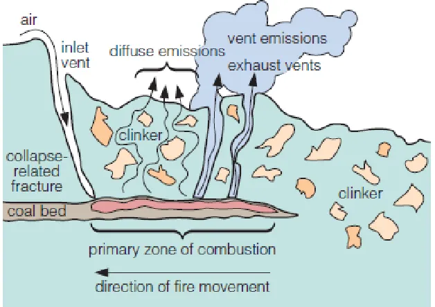
The conceptual model for coal mine fire vent emission is given in Figure 2. Independent research workers in the USA measured the presence of CH4, CO2, CO, and Hg within vents

from U.S. surface coal fires (0–50 °C) (

Hower et al., 2009

) by using exit gas velocity

techniques. Investigators used by S-type pitot tube (

Klopfenstein, 1998

) attached to a flow

meter to measure the range of gas velocities from the coal-fire vents. The emission factor (E) for each species of gas exhaled from a coal gas vent was calculated using (Equation 4) (

O'Keefe et al., 2010

):

Ej = Cj× V × A

(

4

)

Where: Ei is the emission of gas component j, Cj - is the concentration of component j in the

vent, V is the average velocity of the gas perpendicular to the vent (assuming the velocity is equivalent for each gas component), and A is cross-sectional area of the vent at the surface.

O’Keefe (

2010

) measured emission 1400tCO2yr-1 at Truman Shepherd fire emissions and

726±72tyr-1_{from seven vents at Ruth Mullins fire suggesting that the fire is consuming about}

250–280tcoalyr-1_{. In another study O’Keefe projected annual CO}₂_{emissions are about} 1000tCO2yr-1, for old smoky fire, Floyd County, Kentucky within the range of previously case

studies. The flux rate for CO2 is 85,000 mg/s/m2 for various vents for two measuring times

(

O'Keefe et al., 2011

). Subsequently, Engle (2011) used a chamber collection method to

(10)

compounds(VOC) using VOC camera snapshot) for CO2 emission (2112 metric tons/year) that

is escaping into the atmosphere from active coal fire region at San Juan Basin, Durango, CO, USA (

Ide and Orr Jr, 2011

).

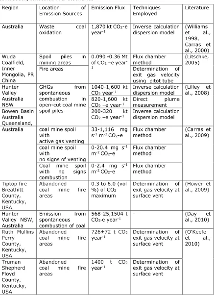
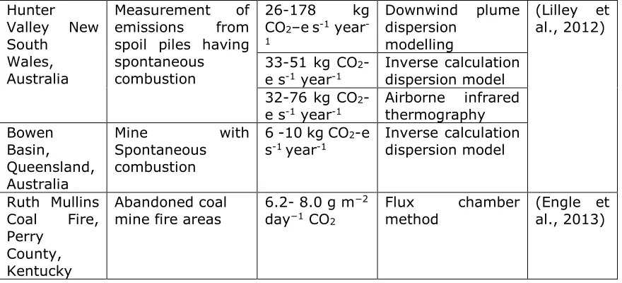
Several studies have been used to quantify emissions from spontaneous combustion/fire/stock piles from coal mines which are summarised in Table 1. However, methodologies are still experimental in this context and requirs focus on developing a robust and practical methodology, equipment for measuring concentration data, sampling regime and modelling techniques. A review of published literature has concluded that there are gaps in the development of a complete inventory of the fugitive GHG emissions experienced from coal mining such as; abandoned surface mines, spontaneous combustion and CO2 in coal

seam gas. Emissions from these sources may be significant for an individual coal mine but it is uncertain as to how significant these emissions may be for an individual country. Countries with data available on CO2 content in their coal mine gas releases should include it with the

sub-category used for the fugitive emissions. GHG measurement methods for emission estimation are designed to study in field investigation for country or basin specific emission factor as per their intensity of spontaneous combustion of coal. The proposed calculation method to estimate the GHG emissions from a typical opencast mine affected by spontaneous combustion is given by the expression:

GHG emission flux = (∑ A × EF × CF

i=n

i=1

) (6)

Where: A – Fire affected area due to spontaneous combustion of coal/fire (m2₎

Emission factor can be calculated by gas released per unit mass of coal in either field investigation or laboratory investigation. The areal extent of the fire affected area may be estimated using either remote sensing techniques and/or observations of site specific conditions. A detailed case study is explained for estimating GHG emissions from two sites of coal fire at Enna Opencast Project Jharia coalfield, India.

3.0 MATERIALS AND METHODS

3.1 Sampling Chamber Used in this Study

(11)

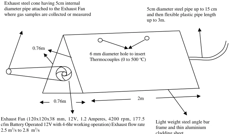
collected within the chamber is removed by a suction fan. The gas flow rates (both inlet and outlet) were recorded by a flow meter. Temperature of the exhaust gas mixture was measured by a thermocouple. The prismatic equilateral triangular chamber was constructed with a light steel inner angle bar frame, clad with a lightweight aluminium sheeting to allow for the ease of disassembly and transport. The equilateral triangular chamber is 2m long (each side of 0.76 m) with an internal volume of 0.5 m3_{, exhaust fan}

(capacity 50 - 100 litremin-1_{), powered by a 12 volt DC battery, a flexible inlet pipe having}

5.0 cm in diameter and 3.0 m in length (Figure 3). The cladding plate joints are sealed by aluminium foil strip and normal packing sticky tape for chamber to be leak proof from all sides except bottom. A series of laboratory and field tests were performed on the collection chamber to evaluate the operation and effectiveness of the: battery capacity, thermocouples, fan capacity, inlet pipe length and diameter, sealing adhesive tapes, exhaust cone in outlet, outlet pipe length,diameter and volume of chamber. The final configuration of the sampling chamber is given in Figure 3.

3.2 Field investigation

3.2.1 Background to Study Area

Field investigations were carried out at two sites located on the Enna Opencast Project which belongs to M/s Bharat Cooking Coal, Ltd (BCCL) of Jharia coal field, Dhanbad, India. The opencast project began operations in 1982-83 following the closure of a number of small underground pits (started in 1906) which practised the bord and pillar method of mining. The project area covers a total surface area of 1.813 km2_{and that is underlain by a number of}

coal seams (from I to XV) in thickness from about 1.21 m to 17.1 m at depths which vary between 40-120 m. The coal seams of leasehold are steep with an average dip amount of 44o

in the direction of south west. The average gradient of seam is 1:9 towards S44W. The stratigraphic sequences of different coal seam at Enna Colliery, JCF, India are shown in Figure 4. The present states of different seams are as follows:

• XV (7.90 m) - Exhausted

• XIV (7.62 m) - Exhausted

• XIII (7.32 m) - Exhausted

• XI/XII (11.0 m) - Opencast mine and seams have active fire

• X (12.8 m) - Developed and Depillared in 3 sections

• IX (1.21 m) - Partially Developed

(12)

• 0 – V Seam - Virgin

Previously partially extracted shallow depth underground mines were liable to spontaneous combustion of the residual roof, pillar and floor coal due to subsidence and the creation of openings, cracks and fractures in the overlying strata which often connects to surface. During the execution of the field study at the mine, opencast coal extraction was confined to the removal of the standing pillars and old abandoned goafs within the XI and XII seams of the old mine workings at depths of 40 to 60m, respectively. In many instances it is not safe to access the land containing these fires due to the high temperatures, and unstable ground conditions. Access to these areas is controlled by the regulations for health and safety of workers operated by the Directorate General Mine Safety (DGMS). Leasehold mining areas may be classified into four categories related to the ground stability conditions and the risk of the spontaneous combustion of coal for the health and safety aspects of miners (Table 2). The experimental site chosen for the field study should be free from: (i) a potential disturbance to current operations and (ii) be contained within a stable and accessible surface area. Fresh coal samples were collected from the X /XI seam that is subject to the active spontaneous combustion/concealed fires in the affected areas. The quality of this coal seam is classified as high grade metallurgical and sub bituminous. The result of the coal analyses performed show a proximate analysis of (M-0.61 %, Ash- 20.94 %, VM- 21.14 %, FC-57.31 %) and an ultimate analysis (C-63.78 %, H2 -3.94 %, N2- 1.27 %, O2-9.46 %). The three

different analytical methods (petrographic study of oxidised coal i.e. morphology of oxidised coal and change in reflectance study before and after oxidation; crossing point temperature Indian method and the sponcomb rig test developed at the University of Nottingham (Mohalik, 2013)) were used to determine the susceptibility of the coal samples to spontaneous combustion. The morphology study of coal concludes that more than 60 % vitrinite are having oxidation rim and change in vitrinite reflectance is positive (>10%). The petrographic study concludes that coal is moderately susceptible. The CPT value of this coal is 169C and CPTCT

from sponcomb rig at university of Nottingham is 231 C which concludes that it is poorly susceptible (Mohalik, 2013).

3.2.2 Experimental Procedure

(13)

fire areas were getting inside the chamber. This SC was kept over two cracks (1st_{- length}

93cm and width 2cm, 2nd_{–length 100 cm and width 4cm) during field study. There are six}

cracks of different length i.e. 2.2 m, 5.4 m, 3.6 m, 2.8 m, 4.5 m and 4.1 m with varying crack width 1 cm to 6 cm. The maximum visible depth of crack in study areas are below 40cm.

Except these cracks there were numbers of cracks visible in study site but cannot be approachable due to unstable ground and fire affected areas. So, GHG emission fluxes for area sources were considered to be uniformly distributed for two different temperature zone i.e. low and medium temperatures neglecting fluctuations in emission. As study area looks like a square having approximately 20 m2_{area and for area sources flux calculation this was} considered.

There are certain assumptions required for dynamic open flux chamber (DOFC) measurement of emission fluxes over soils. Similar study was also carried out for other areas of research like gas emission flux measurement from soil/ landfill area by various researches (Zhang et al., 2002, Gao and Yates, 1998b, Gao and Yates, 1998a, Gustin et al., 1999). The steady state gas emission flux, F, (i.e. mass/unit area/time) was calculated from Equation 3 which is used by Carras et al (2009). The schematic diagram (Figure 6) and theoretical assumptions for dynamic open flux chamber (DOFC) were summarised as follows:

a. Co(t)=Ca(t), i.e., the outlet gas concentration measured represents the actual internal

SC gas concentration. This requires sufficient internal mixing, an outlet line as short as possible, and no chemical changes of sampled gases in DOFC or outlet line. This assumes that sufficient internal mixing takes place regardless of the DOFC design.

b. Cs(t)=Cs. This assumes a constant, uniform gas emission source with a uniform surface

distribution because of fire in opencast mines. Ventilation did not play any role for combustion whereas wind pressure and velocity plays role.

c. The exhaust flow rate (Qi and Qo) is constant and achievable with a uniform velocity

from inlet to outlet at any given time.

d. Exhaust flow rate does not cause any internal pressure deficit (internal vacuum) or surplus, which excludes any “pumping effect”. The inlet and outlet diameter are kept same to minimise this effect.

(14)

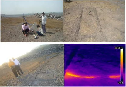
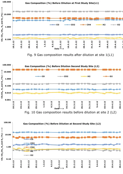
The chamber was placed over the cracks selected for survey for 5 minutes to allow the gases exiting the covered cracks and vents to fill up the chamber. A sample of the gas and its temperature were collected at the inlet and outlet to the chamber to determine the initial and final concentrations of the gases entering and leaving the chamber (Figure 7). Three complementary analytical techniques were used to determine the concentration of the sampled gas mixtures entering and exiting the DOFC. These included a manual chemical based analysis, a hand held multi gas analyser, and gas chromatography to cross check a selection of the manual samples collected. The collected air samples were analysed continuously by a multi gas analyser (MX6 manufactured by MS Industrial Scientific Limited, USA). Unfortunately, due to the low concentrations of some of the gases species in the collected samples, the instrument was unable discriminate to a sufficient accuracy the presence of these species. To supplement these potentially deficient gas sample analyses, an additional set of gas samples were manually collected by employing an aspirator and suction tube. These samples were collected in evacuated nylon gas collector bags. The exit velocity of the outlet gases was measured using digital anemometer. The manually collected gas samples were taken three times to confirm the repeatability of the experimental method. These field study measurements were carried out over the same two cracks over a three month period, which permitted a collection of a total of 40 individual sets of repeated samples. The concentrations of the species of the gases within these samples were subsequently determined in the laboratory by performing a combination of a manual chemical analysis and gas chromatography. The results of product of combustion gases (i.e. CO, CO2,

CH4, H2 and O2) before and after measurement from two different field sites are given in

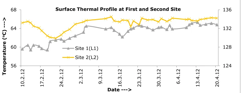
Figure 8- 11. The temperature of the mixing gases inside the DOFC were measured using thermocouples, these temperatures were further confirmed by the intermittent use of thermal imaging camera available during the field study (Figure. 7 b, c & d). Similarly, ambient temperature and ground temperature over crack zone were measured before each day experiment to know temperature variation of the site. The average temperature of the exhaust gases measured at cracks 1 and 2 were 42.6 and 54.05 C, respectively. Whereas, the variation in the actual ground temperature measured by the thermocouples at the two sites for whole study period was between 63±4C and 133±4C, respectively (Figure. 12). Subsequently, the field sites 1 and 2 were classified as the low and medium strata temperature zones.

(15)

The GHGs from spontaneous combustion / coal mine fires is usually diluted with air as it exits and transfuses away from mines due to temperature inversions or other meteorological conditions, resulting in a potential health hazard in populated areas. In this case study, chamber measurement was carried out over a surface cracks, which is a line source. So the expression for flux will be (Equation 7):

𝐹𝑙𝑢𝑥 (𝐹𝑡𝐿) = 𝑄 × (𝐶𝑜 − 𝐶𝑖)/𝐿 (7)

Where; L – Length of cracks (m)

As the concentrations of all of the gas species present are determined in ppm or as a general body concentration in air (%), these concentration may be converted to a mass flux (gm/s) assuming the temperature of the measured gas emission and standard atmospheric pressure. The average emission rates determined from the two selected emission sites are summarised in Table 3. The average gas fluxes (determined from the analysis of the collected 40 sets of data) recorded the flux rates or each of the different measured gas species over a time scale of between 1 to 90 days (which were used to determine the average cumulative emission fluxes). The assumptions for these calculations, were that all measurements was recorded at a standard atmospheric (P) - 101325 Pa and at the field measured gas emission temperatures. To form the cumulative average emission fluxes, an average of 25 individual measurements were used. The emission fluxes measured at the two sites and their standard error means are presented in Table 3. If all of these line sources (L1, L2, L3, L4, L5 and L6) are classified as low

temperature sources. Consequently, this region was classified as a low temperature combustion zone. Similarly, all of the lines in the vicinity of the line 2 study area (L’1, L’2, L’3,

L’4, L’5 and L’6) may be defined as medium temperature sources, and this area termed a

medium combustion zone. The average gas fluxes determined from the areal measurement of the different measured gases within the low and medium temperature combustion zones are given by equations 8 and 9:

Flux for low temperature zone

The results from this study provide a benchmark for estimating the GHGs that issue from individual cracks observed at a surface coal mine. However, determination of the crack location, dimension and classification of all of the cracks and vents that may exist at an affected mine presents a major challenge. This emission data may be used to project the emissions expected across other identified areas of the mine affected by spontaneous combustions. As an illustration this data was subsequently used to provide a first estimate to the emissions expected from a 500 m2_{of land area within a mine property experiencing}

combustion emissions. Consequently, it is determined that the total GHG emissions ( CO2

equivalent) from this single fire affected mines of JCF assuming similar contribution of area emission above and taking minimum (low temperature - 60 o_{C surface temperature) and}

maximum concentration (medium temperature – 130 o_{C surface temperature) (1 kg CH}₄_{= 21}

kg of CO2) releases:

500x2673.26+ 500x1478.50*21  16.86 Mtyr-1_±6.65%

500x10192.76+ 500x1437.40*21  20.19 Mtyr-1_±10.58%

The exact quantification of the extent of the active coal fires across the JCF is not currently possible due to the lack of available data. However, first order estimates that scope the upper and lower level value of GHG emissions may be obtained by the extrapolation of the results obtained from the field studies reported above.

Currently, the JCF is spread over a geological area of 450 km2_{that contains an estimated coal}

bearing area of over 350 km2_{. Presently, BCCL holds the major leasehold of 273 km}2_{; Tata}

Iron Steel and Company (TISCO) own a further 22 km2_{and the Steel Authority of India Limited}

(SAIL) own an additional 10 km2_{of the mineral rights (Jain et al., 2011). The 2008, Central}

Mine Planning and Design Institute Limited (CMPDIL) master plan approved by the Government for the JCF indicated there were 67 active fires covering an area of 8.90 km2

operated by BCCL(CMPDIL, 2006). In addition, there were other fire affected areas at overburden dumps, coal stocks and coal washery reject dumps and lagoons(Pandey et al., 2013). There were also a small number of fires recorded on the mineral properties operated by both TISCO and SAIL. The classification of property as one affected by fire, does not necessarily imply that the total area of that property is subject to active fires. From observation it is assumed that 10% of the surface area of property is affected by fires (1:10 km2_{) and that one percent of the fire affected area (say i.e. 0.0089 km}2_{= 8900 m}2_{) is covered}

(17)

dimensions and thermal signatures then the annual total emissions from the JCF. may vary between 300±6.62%to 359±10.55%- MTyr-1_{of CO}₂_{gas equivalents.}

There are other mature Indian coalfields like the Raniganj and Wardha coalfields, and the Godavari basin and the Mahanadi coalfields that have over the past four decades experienced fire problems(Mohalik et al., 2009). However, the characteristics of these fire affected areas in these coalfields are not similar to those that occur in the JCF. If we further assume another 1 km2_{of area in these coalfields are affected by fire and that one percentage of the fire}

affected areas (say 0.01 km2_{) emit GHGs; then total annual GHG emission rate from the}

remaining Indian coalfields may be approximated to vary between 337±6.62%to 403±10.56%4Mtyr-1_{of CO}₂_{gas equivalents. Thus, the total annual national contribution to}

the GHG budget made by the spontaneous combustion of coal may be estimated to vary from between 637±6.62%- to 763±10.56%- Mtyr-1_{of CO}₂_{gas equivalents. A recent government}

ministry officially published Indian GHG inventory, estimated the total GHG emissions in 2007 to be 1904.73 Mt of CO2 equivalents (MOEF, 2010). If we assume both lower and upper limit

of above GHG emissions released from spontaneous combustion of coal/concealed fires in India then it may be estimated that these emissions contribution between 33 to 40 % of total national GHG emission.

5.0 CONCLUSIONS

The estimation of GHG emission due to spontaneous combustion of coal is a major challenge. A systematic study conducted at field conditions may afford a potential solution to problem. The successful quantification of GHG emissions from spontaneous combustions was experienced at site specific conditions. The regional or worldwide scale of GHG emission depend upon several factors i.e. temperature, dimensional variation, coal characteristics and geo-mining conditions.

An attempt has been made to estimate GHG emissions from spontaneous combustion of coal for the first time in India. In this study two field measurements were carried out to evaluate direct measurement technique (Sampling chamber method) of GHGs emitted from an active spontaneous combustion coal seam at Enna Opencast Project, Jharia coalfield (JCF) for three months. The study reveals that emission of CO2 varies 75.02 to 286.03 gs-1m-1 and CH4 varies

41.49 to 40.34 gs-1_m-1 _{respectively for low and medium temperature zone. The results from}

(18)

-1_{of CO}₂_{gas equivalents. It concludes that the emissions are scaled by their size and location}

(19)

REFERENCES

BELL, F. G., BULLOCK, S. E. T., HÄLBICH, T. F. J. & LINDSAY, P. 2001. Environmental

impacts associated with an abandoned mine in the Witbank Coalfield, South Africa.

International Journal of Coal Geology,

45 ,

195-216.

CARRAS, J. N., DAY, S. J., SAGHAFI, A. & WILLIAMS, D. J. 2009. Greenhouse gas emissions

from low-temperature oxidation and spontaneous combustion at open-cut coal mines in

Australia.

International Journal of Coal Geology,

78 ,

161-168.

CARRAS, J. N., DAY, S. J., SZEMES, F., WATSON, J. A. & WILLIAMS, D. J. 2002. Airborne

infrared thermography as a method for monitoring spontaneous combustion and

greenhouse gas emissions.

ACARP Project C9062 Final Report, Brisbane: Australian Coal

Association,

41. CHATTERJEE, R. S. 2006. Coal fire mapping from satellite thermal IR data - A case example in

Jharia Coalfield, Jharkhand, India.

ISPRS Journal of Photogrammetry and Remote Sensing,

60 ,

113-128.

CMPDIL, R. 2006. Bharat Coking Coal Limited (BCCL) Master plan 2008 for “Dealing with

Fires, Subsidence and Rehabilation in the leasehold of BCCL”

Central Mine Planning

Design Institute Limited Report

.

DHAR, B. B. 1996. Keynote address on status of mine fires – Trends and challenges.

In

Proceedings of the Conference on Prevention and Control of Mine and Industrial Fires -

Trends and Challenges, Calcutta, India,

1-8.

EGGLESTON, S., BUENDIA, L., MIWA, K., NGARA, T. & TANABE, K. E. 2007. 2006 IPCC

Guidelines for National Greenhouse Gas Inventories.

IGES, Japan. Prepared by the

National Greenhouse Gas Inventories Programme, ,

5. ENGLE, M. A., OLEA, R. A., HOWER, J. C., STRACHER, G. B. & KOLKER, A. 2012a.

Methods to quantify diffuse CO2 emissions from coal fires using unevenly distributed flux

data. .

In: Stracher, G.B., Prakash, A., Sokol, E.V. (Eds.), Coal and Peat Fires: a Global

Perspective, Elsevier, Amsterdam

2 ,

24. ENGLE, M. A., OLEA, R. A., O'KEEFE, J. M. K., HOWER, J. C. & GEBOY, N. J. 2012b. Direct

estimation of diffuse gaseous emissions from coal fires: Current methods and future

directions.

International Journal of Coal Geology

.

ENGLE, M. A., RADKE, L. F., HEFFERN, E. L., O'KEEFE, J. M. K., SMELTZER, C. D.,

HOWER, J. C., HOWER, J. M., PRAKASH, A., KOLKER, A., EATWELL, R. J., TER

SCHURE, A., QUEEN, G., AGGEN, K. L., STRACHER, G. B., HENKE, K. R., OLEA,

R. A. & ROMÁN-COLÓN, Y. 2011. Quantifying greenhouse gas emissions from coal fires

using airborne and ground-based methods.

International Journal of Coal Geology,

88 ,

147-151.

GANGOPADHYAY, P. K. 2007. Application of remote sensing in coal-fire studies and coal-fire–

related emissions.

Reviews in Engineering Geology,

18 ,

239-248.

GAO, F. & YATES, S. R. 1998a. Laboratory study of closed and dynamic flux chambers:

Experimental results and implications for field application.

Journal of Geophysical

Research: Atmospheres,

103 ,

26115-26125.

(20)

GUSTIN, M., RASMUSSEN, P., EDWARDS, G., SCHROEDER, W. & KEMP, J. 1999.

Application ofa laboratory gas exchange chamber for assessment of in situ mercury

emissions.

Journal ofGeoph ysical Research

104 ,

21873-21878.

HEFFERN, E. L. & COATES, D. A. 2004. Geologic history of natural coal-bed fires, Powder

River basin, USA.

International Journal of Coal Geology,

59 ,

25-47.

HOWER, J. C., HENKE, K., O'KEEFE, J. M. K., ENGLE, M. A., BLAKE, D. R. & STRACHER,

G. B. 2009. The Tiptop coal-mine fire, Kentucky: Preliminary investigation of the

measurement of mercury and other hazardous gases from coal-fire gas vents.

International

Journal of Coal Geology,

80 ,

63-67.

IDE, S. T. & ORR JR, F. M. 2011. Comparison of methods to estimate the rate of CO2 emissions

and coal consumption from a coal fire near Durango, CO.

International Journal of Coal

Geology,

86 ,

95-107.

JAIN, M. K., PAUL, B. & RAJU, E. V. R. 2011. Jharia coalfield a retrospection

Minenvis,

69 &

70 ,

6. JENNIFER, M. K. O. K., HENKE, K. R., HOWER, J. C., ENGLE, M. A., STRACHER, G. B.,

STUCKER, J. D., DREW, J. W., STAGGS, W. D., MURRAY, T. M., HAMMOND III,

M. L., ADKINS, K. D., MULLINS, B. J. & LEMLEY, E. W. 2010. CO2, CO, and Hg

emissions from the Truman Shepherd and Ruth Mullins coal fires, eastern Kentucky, USA.

Science of The Total Environment,

408 ,

1628-1633.

KIM, A. G. 2007. Greenhouse gases generated in underground coal-mine fires.

Reviews in

Engineering Geology,

18 ,

1-13.

KLOPFENSTEIN, R. J. 1998. Air velocity and flow measurement using a pitot tube.

ISA

Transactions,

37 ,

257-263.

KUENZER, C., ZHANG, J., LI, J., VOIGT, S., MEHL, H. & WAGNER, W. 2007a. Detecting

unknown coal fires: synergy of automated coal fire risk area delineation and improved

thermal anomaly extraction.

Int. J. Remote Sens.,

28 ,

4561-4585.

KUENZER, C., ZHANG, J., TETZLAFF, A., VAN DIJK, P., VOIGT, S., MEHL, H. &

WAGNER, W. 2007b. Uncontrolled coal fires and their environmental impacts:

Investigating two arid mining regions in north-central China.

Applied Geography,

27 ,

42-62.

MOEF 2010. Indian network of climate change assessment (INCCA), India’s greenhouse gas

emissions 2007.

Ministry of Environment and Forests, Government of India, 2010

.

MOHALIK, N. K. 2013. A study of the sponaneous heating of Indian coals.

PhD thesis,University

of Nottingham, Nottingham, UK.

MOHALIK, N. K., SINGH, R. V. K., SINGH, V. K. & TRIPATHI, D. D. 2009. Critical Appraisal

to Assess the Extent of Fire in Old Abandoned Coal Mine Areas - Indian Context.

in Aziz,

N (ed), Coal 2009: Coal Operators' Conference, University of Wollongong & the

Australasian Institute of Mining and Metallurgy,,

271-280.

NOLTER, M. A. & VICE, D. H. 2004. Looking back at the Centralia coal fire: a synopsis of its

present status.

International Journal of Coal Geology,

59 ,

99-106.

(21)

O'KEEFE, J. M. K., NEACE, E. R., LEMLEY, E. W., HOWER, J. C., HENKE, K. R., COPLEY,

G., HATCH, R. S., SATTERWHITE, A. B. & BLAKE, D. R. 2011. Old Smokey coal fire,

Floyd County, Kentucky: Estimates of gaseous emission rates.

International Journal of

Coal Geology,

87 ,

150-156.

PANDEY, J., D. KUMAR, R.K. MISHRA, N. K. MOHALIK, A. KHALKHO & V. K. SINGH

2013. Application of Thermography Technique for Assessment and Monitoring of Coal

Mine Fire: A Special Reference to Jharia Coal Field, Jharkhand, India, .

International

Journal of Advanced Remote Sensing and GIS,

2 ,

138-147.

PONE, J. D. N., HEIN, K. A. A., STRACHER, G. B., ANNEGARN, H. J., FINKLEMAN, R. B.,

BLAKE, D. R., MCCORMACK, J. K. & SCHROEDER, P. 2007. The spontaneous

combustion of coal and its by-products in the Witbank and Sasolburg coalfields of South

Africa.

International Journal of Coal Geology,

72 ,

124-140.

PRAKASH, A. & GUPTA, R. P. 1998. Land-use mapping and change detection in a coal mining

area - a case study in the Jharia coalfield, India.

International Journal of Remote Sensing,

19 ,

391-410.

SHEAIL, J. 2005. ‘Burning bings’: a study of pollution management in mid-twentieth century

Britain.

Journal of Historical Geography,

31 ,

134-148.

STRACHER, G. B. 2004. Coal fires burning around the world: a Global Catastrophe.

International

Journal of Coal Geology,

59 ,

1-6.

STRACHER, G. B. & TAYLOR, T. P. 2004. Coal fires burning out of control around the world:

thermodynamic recipe for environmental catastrophe.

International Journal of Coal

Geology,

59 ,

7-17.

TETZLAFF, A. 2004. Coal fire quantification using Aster, ETM and Bird instrument data.

Thesis,

Ludwig Maximilians University, Munich,

155. VAN DIJK, P., ZHANG, J., JUN, W., KUENZER, C. & WOLF, K.-H. 2011. Assessment of the

contribution of in-situ combustion of coal to greenhouse gas emission; based on a

comparison of Chinese mining information to previous remote sensing estimates.

International Journal of Coal Geology,

86 ,

108-119.

WHITEHOUSE, A. E. & MULYANA, A. A. S. 2004. Coal fires in Indonesia.

International

Journal of Coal Geology,

59 ,

91-97.

ZHANG, H., LINDBERG, S. E., BARNETT, M. O., VETTE, A. F. & GUSTIN, M. S. 2002.

Dynamic flux chamber measurement of gaseous mercury emission fluxes over soils. Part

1: simulation of gaseous mercury emissions from soils using a two-resistance exchange

interface model.

Atmospheric Environment,

36 ,

835-846.

ZHAO, Y., ZHANG, J., CHOU, C.-L., LI, Y., WANG, Z., GE, Y. & ZHENG, C. 2008. Trace

element emissions from spontaneous combustion of gob piles in coal mines, Shanxi, China.

International Journal of Coal Geology,

73 ,

52-62.

(22)

[image:22.612.128.482.99.298.2] [image:22.612.149.463.343.565.2]

Fig. 1 Schematic diagram of the large chamber used to measure gas flux from spoil piles and other surfaces (Source: Carras et al., 2009)

(23)

[image:23.612.89.469.85.308.2]

Fig. 3 Final design of scientific sampling chamber for field study (Not to scale)

5cm diameter steel pipe up to 15 cm and then flexible plastic pipe length up to 3m.

Exhaust Fan (120x120x38 mm, 12V, 1.2 Amperes, 4200 rpm, 177.5 cfm Battery Operated 12V with 4-6hr working operation) Exhaust flow rate 2.5 m3_{/s to 2.8 m}3_/s

0.76m

2m 0.76m

Light weight steel angle bar frame and thin aluminium cladding sheet.

6 mm diameter hole to insert Thermocouples (0 to 500 o_C) Exhaust steel cone having 5cm internal

(24)

[image:24.612.77.488.112.251.2]

Fig. 4 The Stratigraphic sequence of different coal seam at Enna Colliery, JCF, India (Not to

scale)

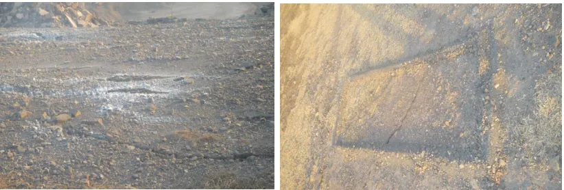
[image:24.612.120.481.305.467.2]

Fig. 5 - Enna OCP, JCF of (a) Unstable fire area (b) Study area

Fig. 6 Conceptual model to determine the GHG fluxes entering dynamic open flux chamber from a measurement of the outlet gas concentrations.

Outlet

C

o(t)

Q

o

Exhaust Air

Air

C

a(t)

F

(t)

Inlet

C

i(t)

Q

i

Ambient Air

(25)

[image:25.612.72.487.71.358.2]

Fig. 7 (a) Gas sample collection (b) Temperature measurement using thermocouple (c) FLIR

Thermocam (d) Thermal Image

Fig. 8 Gas composition results before dilution at site 1 (L1)

0.001 0.010 0.100 1.000 10.000 100.000 1 0 .2 .1 2 1 5 .2 .1 2 2 0 .2 .1 2 2 5 .2 .1 2 1 .3 .1 2 6 .3 .1 2 1 1 .3 .1 2 1 6 .3 .1 2 2 1 .3 .1 2 2 6 .3 .1 2 3 1 .3 .1 2 5 .4 .1 2 1 0 .4 .1 2 1 5 .4 .1 2 2 0 .4 .1 2 C O , C O2 H2, a n d O 2 (% ) ----> Date --->

Gas Composition (%) Before Dilution at First Study Site(L1)

CO CO2

[image:25.612.76.480.460.604.2]

(26)

[image:26.612.73.479.74.648.2]

Fig. 9 Gas composition results after dilution at site 1(L1)

Fig. 10 Gas composition results before dilution at site 2 (L2)

Fig. 11 Gas composition results after dilution at second study site 2(L2)

0.100 1.000 10.000 100.000 1 0 .2 .1 2 1 5 .2 .1 2 2 0 .2 .1 2 2 5 .2 .1 2 1 .3 .1 2 6 .3 .1 2 1 1 .3 .1 2 1 6 .3 .1 2 2 1 .3 .1 2 2 6 .3 .1 2 3 1 .3 .1 2 5 .4 .1 2 1 0 .4 .1 2 1 5 .4 .1 2 2 0 .4 .1 2 C O , C O2 , C H4 , H2 a n d O 2 (% ) ----> Date --->

Gas Composition (%) Before Dilution at First Study Site(L1)

CO CO2 CH4 H2 O2

0.001 0.010 0.100 1.000 10.000 100.000 1 0 .2 .1 2 1 5 .2 .1 2 2 0 .2 .1 2 2 5 .2 .1 2 1 .3 .1 2 6 .3 .1 2 1 1 .3 .1 2 1 6 .3 .1 2 2 1 .3 .1 2 2 6 .3 .1 2 3 1 .3 .1 2 5 .4 .1 2 1 0 .4 .1 2 1 5 .4 .1 2 2 0 .4 .1 2 C O ,C O2 , H 2 a n d O 2 (% ) ----> Date --->

Gas Composition (%) Before Dilution Second Study Site (L2)

CO CO2 H2 O2

0.10 1.00 10.00 100.00 1 0 .2 .1 2 1 5 .2 .1 2 2 0 .2 .1 2 2 5 .2 .1 2 1 .3 .1 2 6 .3 .1 2 1 1 .3 .1 2 1 6 .3 .1 2 2 1 .3 .1 2 2 6 .3 .1 2 3 1 .3 .1 2 5 .4 .1 2 1 0 .4 .1 2 1 5 .4 .1 2 2 0 .4 .1 2 C O , C O2, CH 4 , H2 a n d O 2 (% ) ----> Date --->

Gas Composition (%) Before Dilution at Second Study Site (L2)

CO

CO2

CH4

H2

[image:26.612.79.485.77.240.2]

(27)

[image:27.612.74.492.75.235.2]

Fig. 12 Thermal profile study using thermocouple at both site (i.e.L1 and L2) 124 128 132 136 56 60 64 68 1 0 .2 .1 2 1 7 .2 .1 2 2 4 .2 .1 2 2 .3 .1 2 9 .3 .1 2 1 6 .3 .1 2 2 3 .3 .1 2 3 0 .3 .1 2 6 .4 .1 2 1 3 .4 .1 2 2 0 .4 .1 2 T e mp e ra tu re ( oC ) ---> Date --->

Surface Thermal Profile at First and Second Site

(28)

Table 1: Review of GHG emission estimation methodology from spontaneous combustion/concealed fire/ stock piles

Region Location of

Emission Sources Emission Flux Techniques Employed Literature

Australia Waste coal

oxidation 1,870 kt COyear-1 2-e Inverse calculation _{dispersion model} (Williams _et _al.,

1998, Carras et al., 2000) Wuda Coalfield, Inner Mongolia, PR China

Spoil piles in

mining areas 0.090 -0.36 Mt of CO2 –e year -1

Flux chamber

method (Litschke, 2005)

Fire areas Determination of

exit gas velocity using pitot tube Hunter

Valley Australia NSW

GHGs from

spontaneous combustion in open-cut coal mine spoil piles

1040-1,600 kt CO2 year-1

Inverse calculation

dispersion model (Lilley et al., 2008) 820-1,600 kt

CO2 –e year-1

Direct plume measurement Bowen Basin

Australia Queensland,

200-320 kt CO2 –e year-1

Inverse calculation dispersion model

Australia coal mine spoil with

active gas venting

33-1,116 mg

s-1_m-2 _CO₂_-e Flux chamber _method (Carras et _{al., 2009)}

coal mine spoil with

no signs of venting

0-20.4 mg s-1

m-2 _CO₂_-e Flux chamber _method

Coal mine spoil with no signs combustion

0-2.4 mg s-1

m-2 _CO₂_-e Flux chamber _method

Tiptop fire Breathitt County, Kentucky, USA Abandoned

coal mine fire areas

0.3 to 6.0 (vol %) of CO2

maximum

Determination of exit gas velocity at surface vent

(Hower et al., 2009)

Hunter Valley NSW, Australia

Emission from spontaneous combustion of coal

568-25,1504 t CO2-e year-1

- (Day et

al., 2010)

Ruth Mullins Perry

County,

Kentucky,

USA

Abandoned

726±72 t CO2

year-1 Determination of _{exit gas velocity at}

surface vent

(O'Keefe et al., 2010) Truman Shepherd Floyd County, Kentucky, USA Abandoned

1400 t CO2

year-1 Determination of _{exit gas velocity at}

[image:28.612.74.513.100.708.2]

(29)

Old Smokey coal fire, Floyd

County, Kentucky

Abandoned coal mine fire areas

85,000 mg s-1

m-2_CO₂ Determination of _{exit gas velocity at}

surface vent

(O'Keefe et al., 2011)

San Juan Basin

Durango, CO, USA

Outcrop fire areas 2112 t year-1

CO2e

Exit gas velocity

using VOC camera (Ide and Orr Jr, 2011) 1954 t year-1

CO2e

Flux chamber method

1616 t year-1

CO2e

Chimney method

Ningxia Coal lost due to mine fire

7.441 Mt of CO2e year-1

Data Collection from mine by and default emission factor using Tier 1 approach

(van Dijk et al., 2011) Wuda

coalfield, Inner Mongolia

2.35 Mt of CO2e (2009)

year-1

Inner Mongolia

8.2 Mt of CO2e

year-1

Xinjiang

province 39 Mt of COyear-1 2e

Welch Ranch, Wyoming, USA

Mine fire areas 1.2±0.2 mg s

-1_m-2_CO₂ Flux _method chamber (Engle et _{al., 2011)}

6.7±0.9 mg s

-1_m-2_CO₂ Determination of _{exit gas velocity at}

surface vent 3.5-4.1 mg s-1

m-2_CO₂

Remote airborne data

measurements Mulga,

Alabama, USA

Spoil pile fires 27-48

mg s

-1

m

-2

_CO

₂

Flux chamber method

Ankney, Wyoming, USA

Outcrop fire areas >0.91±0.24 mg s-1_m-2 _CO₂

Flux chamber

method (Engle et al., 2012c) >1.6±0.09 mg

s-1_m-2 Determination of _{exit gas velocity at}

surface vent 12.9-27.1 mg

s-1_m-2 Remote airborne _data

measurements Hotchkiss,

Wyoming USA

Mine Fire areas 4.0±0.48 mg s-1_m-2_CO₂

Flux chamber method Emhlahleni (Witbank) South Africa Measurement of emissions from waste coal piles surface and abandoned coal mines

1,950 000 ± 350,000 t CO2

–eyear-1

Rigid

polycarbonate chambers placed on the ground to measure

emissions. a unit created from half of a 220 litre plastic drum,

(30)

Hunter Valley New South

Wales, Australia

Measurement of emissions from spoil piles having spontaneous combustion

26-178 kg CO2–es-1 year -1

Downwind plume dispersion

modelling

(Lilley et al., 2012)

33-51 kg CO2

-e s-1_year-1

Inverse calculation dispersion model 32-76 kg CO2

-e s-1_year-1 Airborne infrared _thermography

Bowen Basin, Queensland, Australia

Mine with

Spontaneous combustion

6 -10 kg CO2-e

s-1 _year-1 Inverse calculation _{dispersion model}

Ruth Mullins Coal Fire, Perry

County, Kentucky

Abandoned coal mine fire areas

6.2- 8.0 g m−2

day−1_CO₂

Flux chamber method

[image:30.612.73.513.72.272.2]

(Engle et al., 2013)

Table 2 – Ground stability classification employed at the Enna Opencast Project

Class 1 Stable There are no cracks and fissures observed across this ground, which is deemed stable. The temperature of the ground is the same as the surrounding ground.

Class 2 Low Unstable (Miners are allowed with Personal

protective equipment)

The ground is slightly un stable due to small number of cracks and fissures. Smoke and gases are observed rising from the affected ground due to spontaneous combustion of coal. The temperature of the surrounding cracks and fissures are less than 200 0_{C. Access to these areas is prohibited on the grounds}

of health and safety. Class 3

Unstable (Miners are restricted)

The ground is un stable due to large number of cracks and fissures. Smoke and gases are observed to issue from the affected ground due to spontaneous combustion of coal/concealed fire. The temperature of surrounding cracks and fissures are less than 500 0_{C. Access to these areas are}

prohibited on the grounds of health and safety Class 4

Highly Unstable (Miners are restricted)

The ground is highly un stable due to large number of cracks and fissures. Smoke, gases and flames are issuing from the affected ground due to open fires. The temperature of surrounding cracks and fissures are more than 500 0_C.

(31)

Table 4: Emission fluxes computed for the different gases flowing from the line sources

Species of Gas Measured

Cumulative Average Measured Areal Emission Rate (Field Site 1) (gs-1_m-1₎

Cumulative Average Measured Areal Emission Rate (Field Site 2) (gs-1_m-1₎

Flux (FtL1) SEM Flux (FtL2) SEM

CO 3.3282 0.0009 17.746 0.01

CO2 75.0164 0.33 286.0269 0.12

CH4 41.4893 0.07 40.3361 0.03

[image:31.612.71.495.305.435.2]

H2 0.1288 0.00004 0.5646 0.0006

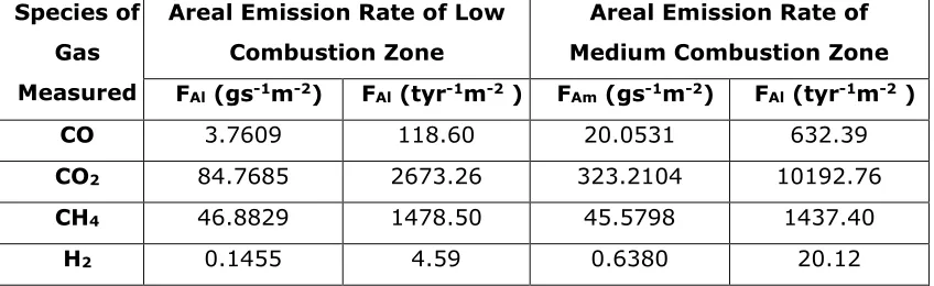
Table 5: The computed gas emission fluxes from the areal sources for the different gas species

Species of Gas Measured

Areal Emission Rate of Low Combustion Zone

Areal Emission Rate of Medium Combustion Zone FAl (gs-1m-2) FAl (tyr-1m-2 ) FAm (gs-1m-2) FAl (tyr-1m-2 )

CO 3.7609 118.60 20.0531 632.39

CO2 84.7685 2673.26 323.2104 10192.76

CH4 46.8829 1478.50 45.5798 1437.40