The Tyranny of Distance and the
Gravity of Resources
Peter E. Robertson
∗The University of Western Australia
Marie-Claire Robitaille
The University of Nottingham Ningbo China
Abstract
To what extent does geography remain an important determinant of compar-ative advantage and factor incomes in resource markets? We estimate gravity models for resources and find that some minerals and fuels, particularly Iron Ore and Gas, do have very high elasticities of trade with respect to distance. To assess the implications of this we then consider a simple counterfactual where location advantages are eliminated. We find that for a few countries, including Australia and New Zealand, distance barriers have a large impact of their market share.
Keywords: Energy, Geography, Gravity Model, International Trade, Re-sources.
JEL: F14, F68, Q02
∗Robertson acknowledges the hospitality of St. Antony’s College Oxford and The Centre for the
1
Introduction
Historically Australia suffered from a “tyranny of distance”. High unit transport costs in shipping wool and wheat to England reduced competitiveness and threatened the eco-nomic viability of the colonies. As Blainey (2001) describes these barriers were mitigated by the sudden availability of large ships during Victorian gold rush, which reduced unit transport costs.1
Likewise, over several centuries, technological improvements in transport have reduced transport cost barriers. Consequently, world manufacturing is characterized by global production networks where country differences in production costs appear to dominate considerations over the distance of markets. Preferences, institutions, and history are now argued to be critical in understanding trade patterns using models of trade in varieties. Conversely the role of endowments as a source of comparative advantage is believed to have been eroded and there is no longer thought to be a “tyranny of distance” caused by prohibitive transport costs (Overman, Redding and Venables 2003, Romalis 2004, Venables 2005, Behrens, Gaign´e, Ottaviano and Thisse 2006, Levchenko 2007, Boulhol and De Serres 2010, Chor 2010).
Nevertheless Australia, and many other southern hemisphere countries, remain largely resource exporters. Resources trade is very different from manufacturing since supply is indelibly linked to a country’s endowments and cannot be relocated or “off-shored”. Moreover, technological advances notwithstanding, many resources, such as iron ore and coal, are bulky and still have relatively high unit transport costs. Others, such as fresh food and gas, have high storage costs. These facts suggest that geography and endow-ments may remain very important factors in explaining the pattern of resources trade and factor returns in resource sectors.
Understanding these issues is important in understanding the impact of taxes and re-source rents on rere-source production. If distance has a large impact on prices faced by consumers, this suggests that a resource company’s country of location may be relatively insensitive to taxes and royalties if any alternative country is very far from the market. This is an important issue for the taxation of resources. For example, with respect to Australia, the government’s ability to tax the iron ore sector in the face of potential competition from Brazil depends on the transport cost margin that Brazil faces in deliv-ering iron ore to the main iron ore market, China. Likewise understanding the impact
1According to Blainey (2001) the inflow of ships carrying prospectors created a supply of cargo ships
of distance on trade patterns is also important for understanding how future changes in technology on transport costs might affect a country’s competitiveness and comparative advantage.
The aim of this paper, therefore, is to quantify the impact of distance – as a measure of geographic isolation – on resources trade patterns. Specifically we estimate the elasticity of trade with respect to distance for different resource commodities and non-manufactured goods. In order to provide some context to these estimates we then consider the predicted world commodity trade patterns if no country had an advantage or disadvantage in terms of geographical location, as measured by distance to markets.
We find that some resource intensive economies’ exports are significantly disadvantaged by their location. For example, we find that the most disadvantaged countries are indeed the southern hemisphere countries – such as Chile, New Zealand, South Africa, Brazil and Australia. For these countries we find that resource exports would be 35-50% higher if their location was at the world average distance from their various resource markets. Thus we find that geography remains very important factor in explaining the global pattern of resources trade and the location decision of firms, and a quantitative understanding of these costs is also important in helping governments make appropriate tax decisions of resource companies.
The remainder of this paper is organized as follows. In Section 2 we discuss the geography of world demand for different commodities. In Section 3 we consider gravity models for food, different raw materials and fuels. Sections 4 and 5 then consider the implications of a counterfactual experiment where distance barriers are equalized across countries and Section 6 concludes.
2
The Geography of World Resources Demand
There are a number of ways to think about how a country’s spatial isolation might affect its trade patterns. Geography affects transport costs but also information costs and political relations, which may in turn translates in trade agreements. There is growing evidence of information, cultural and institutional barriers to trade (Head and Mayer 2013, Kalnins and Lafontaine 2013, Allen 2014).
large fraction of the unit costs. Second, unlike manufacturing, the location of resource supply is largely determined by nature. This means that there are large exogenous differences in the distance between the sources of supply and demand. This contrasts with manufacturing where stages of production can readily be shifted as transport costs rise or fall, as is evident from the global fragmentation of manufacturing production in recent decades. As noted by Blainey (2001), the freight costs of ideas, which are relevant to manufacturing, are cheap but the cost of distance in terms of commodities has been unusually high.
To gain a sense of this dispersion between sources of supply and word demand in resource markets our first task is to characterize the geography of world demand patterns for resources. This differs substantially by commodity. For example, although the USA is the world’s largest importing country overall, China is the world’s largest importer of Minerals followed by Japan. Likewise, with respect to Coal, Japan is by far the largest importer accounting for almost a quarter of world import demand while China is only the 10th largest country, behind countries like Italy and India.
Table 1 summarizes the import shares for selected resource commodities based on COM-TRADE/WITS data, following the Standard International Trade Classification 1 (SITC-1), for 2006. The commodities have been classified into broad categories, that is, Food, Raw Materials, Minerals, Coal, Petrol, and Gas. Given its importance in world trade, and for Australia, we also estimate a model for Iron Ore. The exact SITC-1 categories included into each element of this classification are presented in Table A.1.
It can be seen that overall world import demand is largest in Europe-Central Asia (44%) followed by roughly equal shares from East Asia (23%) and North America (22%).2
However, with respect to Minerals, world import demand is roughly split between Europe-Central Asia (38%) and East Asia (46%). Within this category world demand for Iron Ore is predominantly from East Asia (70%), of which China alone accounts for two thirds (48%). Thus East Asia’s world share of Minerals imports is more than twice as large as its overall world import share while in North America’s Minerals import share is a mere third of its overall world import share.
Likewise world Coal demand is mostly split geographically between East Asia and Europe-Central Asia, with relatively little demand from North America. However, for Gas and Petroleum, world demand is more evenly divided between Europe-Central Asia (35 and 36%), North America (27 and 25%) and East Asia (29 and 29%).
Thus world import demand is somewhat centered on East Asia for Minerals, especially Iron Ore, and for Coal. Conversely North American demand for these same commodities is relatively small. With respect to fuels other than Coal, however, world import demand shifts toward North America. Europe and Central Asia, in contrast, has a very large demand for Food, but relatively little demand for Minerals, except Coal.
To what extent, therefore, does geography determine world trade patterns in these re-sources? One way of addressing this is to consider what the world pattern of trade would be if there was no location advantage or disadvantage for any country. This is our aim in the rest this paper.
[Table 1 about here]
3
The Gravity Model
3.1
A Simple Supply Side Model of the Impact of Distance on
Resources trade
The gravity model is widely used as a description of manufacturing trade and is typically motivated by CES “love of variety” preferences (Anderson and van Wincoop 2003). This setting is less appropriate for resources trade, however, since resource commodities are relatively homogeneous and trade patterns will differ depending on endowments. As explained by Deardorff (1995), other models, including the standard Heckscher-Ohlin model, can also generate gravity relationships. In particular, as noted by Anderson and van Wincoop (2003), the aim of the literature is to develop operational models with a simple form. In this spirit consider a heuristic model of resources supply and transport costs and show how this generates a gravity relationship.
To fix ideas suppose that there are many resource exporting firms, which may be located in one or more export countries. Each export country’s resource sector is characterized by price taking firms exporting to one of n identical export markets. Firms face increasing marginal costs of resource extraction and transport costs that depend upon the distance to the export market. For parsimony suppose that each firm owns one ‘mine” and sells resources to one export market.3 Each firm in country i thus has a unique destination
3The simplifying assumption is for analytical tractability only and is in keeping with many models
index j and the output of each firm is thus given by xi,j.
With free entry each representative firm in country i exporting to country j will satisfy the following zero profit condition,
ai xβi,j Ti,j ≥p¯ (1)
where: ai is a country sector specific (inverse) productivity coefficient; ¯p is the world price, Ti,j is the transport cost mark-up facing firm in country i exporting to country
j, and β > 0 is the elasticity of marginal cost with respect to output. If the inequality is strict then this representative firm shuts down and country i does not export this resource commodity to country j. Thus this competitive model readily permits the zero trade flows that are a ubiquitous feature of the resources trade data.
Since each firm only sells to one marketxi,j is also total exports of this particular resource commodity from country i to country j. Hence we can rearrange equation (1) to obtain the firm’s supply function as
xi,j = ¯p 1
β(a
i Ti,j)−1 (2)
Country i’s total exports of this particular resource are thus given by summing across the destination marketsj.
n
X
j=1
xi,j ≡xi = ¯
pβ1 T˜
i
ai
(3)
where ˜Ti ≡
Pn j=1T
−1
i,j . Combining (2) and (3), we can then obtain country j’s share of countryi’s exports, xi.
xi,j/xi = (Ti,j/T˜i)−1 (4)
Next we note that from the definition of GDP we also have
xi =
αi Yi ¯
p (5)
Substituting (5) into (4) and letting the transport costs take the usual iceberg form
Ti,j =dσi,j, gives
xi,j =γi
Yi ¯
p d −σ
i,j (6)
where γi ≡αi/Pnk=1d−i,kσ is an export country specific constant.
This model, though highly stylized, captures some interesting features of resources trade that differ from the usual monopolistic competition models of trade with CES “love of variety” preferences.4 First, since goods are homogeneous, and firms are small, the
exports sales of one firm do not affect the prices of other countries exports. Thus the usual multilateral price index terms are absent in (6). These indices are often accounted for in empirical work by using destination and export country fixed effects. In (6), however, the export country fixed effect represents the output share of the exporting country’s resource sector, αi, which are attributed, in part, to differences in output shares that may result from differences in resource endowments, as well as differences in technology.
Second the model provides a natural interpretation of the many zero trade flows observed in the data. This is a generic issue in the gravity model literature and is heightened in the case of resources trade. For example, in our sample, there is no trade in Minerals for 61% of the country-pair-year observations. The equivalent number for manufacturing is only 18%. In what follows therefore we employ the Santos Silva and Tenreyro (2006) specification of the gravity model which handles the numerous zero trade flow observa-tions in a parsimonious way that is consistent with the shutdown condition arising as volumes get very small.
3.2
Estimation Strategy and Data
Our data set is constructed from COMTRADE/WITS yearly data for the 104 economies for which all variables are available, following the SITC-1 classification for the period 1998-2003 and 2006.5 We use import data to measure trade flows between country-pair
4It may be emphasised that this model focuses on the supply side, and ignores the demand side.
This therefore ignores possible general equilibrium interactions treats prices and incomes as given. This mirrors the standard approach which treats supply costs as given and assumes linear production func-tions. Naturally in fact there would also however be more complex general equilibrium reactions and this model simply focuses on the primary impact on trade.
5As in Greenaway, Mahabir and Milner (2008), we include Hong Kong’s exports with China’s exports
as imports data are believed to be less at risk of double-counting and misreporting of the country of origin/destination than exports data (Athukorala 2009).
There are two problems with the traditional log-linearization of the gravity model equa-tion. The first is that the data usually contain many zero values. This may arise from missing values or represent genuine instances of zero trade between country-pairs. As noted above this is an important consideration is resources trade.
The common solution of omitting the zero trade observations leads to selection bias (Santos Silva and Tenreyro 2006, Disdier and Head 2008). Santos Silva and Tenreyro (2006) also point out that the log linearization of the gravity equation leads to biased co-efficient estimates in the presence of heteroscedasticity. They propose the use of a Poisson Pseudo-Maximum-Likelihood (PPML) model which, by avoiding log-linearization, thus avoids the problem of zeroes and bias.6
Thus following Santos Silva and Tenreyro (2006), we estimate the gravity model using the PPML estimator.
xci,j,t =δ0cYδc1 i,tY δc 2 j,tN δc 3 i,tN δc 4 j,tA δc 5 i,jD δc 6 i,jH deltac 7 i,t H δc 8 j,te
ζc0G+θc0Fνc
i,j,t (7)
where xci,j,t is the trade volume, in constant $USm, between exporting country i and importing country j for commodity c in year t, δc
0 is a constant, δc1 to δ8c are coefficients
to be estimated, Gis a 7x1 vector of dichotomous variables, F is a 250x1 vector of fixed effects, ζc and θc are, respectively, a 7x1 and a 250x1 vector of coefficients and νc
i,j,t is the error term.
Yi,t and Yj,t are the GDP of the exporting and the importing country, respectively; Ni,t and Nj,t the population of the exporting and importing country, respectively; Ai,j the land area of the country-pair. Di,j stands for the weighted great-circle distance between the country-pair, with the weight depending on the population distribution within both
labour from China. Also note that some countries do not report every year. Thus our strategy is to maximize the number of large natural resources exporters and have a highly representative sample of countries.
6An alternative approach is to use the Tobit model. However, as pointed out by Linders and Groot
partner countries.7 H
i,t and Hj,t are the human capital level in the exporting and im-porting country, respectively.8
The vector G is composed of a set of dummy variables classifying the pair of country as none is landlocked (reference category), one country is landlocked (L1i,j) and two countries are landlocked (L2i,j) and a dummy variable taking the value of one if the two countries in the country-pair are contiguous (Si,j), a set of dummy variables classifying the country-pair into none of the countries is an island (reference category), one country in the country-pair is an island (I1i,j), and the two countries in the country-pair are islands (I2i,j), a dummy variable for language, which takes the value of one if at least one language is spoken by at least 9% of the population in both countries (Ei,j) and a dummy variable taking the value of one if the two countries in the country-pair have ever been in a colonial relationship (Ci,j).
Finally, the vector F is a set of fixed effects for exporting countries (γi), for importing countries (γj) and for years (dt) are included.9 The standard errors are adjusted for clustering at the country-pair level.
Thus we estimate the impact of geographical remoteness as measured by distance which will include transport costs and other factors such as information and cultural barriers. Nevertheless there may also be effects of culture and language that are independent of geographical separation. For example the UK and the USA are distant but share a language, while France and UK are close but have different languages. Thus the inclusion of the common language and colonial link variables is designed to control for these types of barriers that are not directly related to the distance between exporter and importer.10
7As a robustness check, all models were re-estimated using the great-circle distance between capital
cities instead of the great-circle distance between major cities weighted by the population share. The results are similar to the one we obtained using the weighted distance for most of our dependent variables, with the exception of gas carried in its gaseous form. For gas carried in its gaseous form, we find that using the unweighted distance reduces significantly the elasticity of trade to distance and bring it almost to par with the elasticity of trade to distance of gas carried in liquefied form (results available on request).
8Human capital is measured using the Mincerian relationshipe0.15s wheres is the average years of
schooling in the labour force (Barro and Lee 2010).
9Country-year fixed effects are generally used in the literature to control for multilateral resistance
terms. As our theoretical model assumes that goods are homogenous and firms are small, we do not have multilateral price index in our model. The theoretical model however calls for country fixed effects as endowments in natural resources are central to explain which countries export natural resources. As we do not have a good measure of natural resources endowments, we control for endowments using country fixed effects. It is however possible that those endowments vary over time, as countries may discover new deposits. As a robustness check we have thus re-estimated the model using exporter and importer country-year fixed effects. Given the large number of dummy variables the model does not converge for coal, iron ore and petrol. The inclusion of these exporter and importer country-year fixed effects does not markedly change the results (which are available on request).
10Nevertheless there are likely to be other unobserved cultural and information barriers. A related
3.3
Trade-Distance Elasticities by Commodity
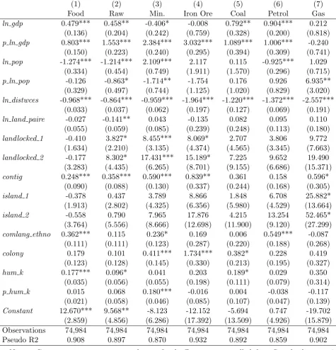
The results are given in Table 2. It can be seen that distance is highly significant for all of the different commodity groups and that the elasticities for the various commodities differ substantially from each other. They range from -0.86 for Raw Materials to -1.96 for Iron Ore and -2.56 for Gas. In general the trade elasticities for Iron Ore and fuels are substantially larger than the elasticities of manufactured goods that are typically reported in the literature.
Interestingly we do not find much evidence than geography matters in other respects than distance and the contiguous border dummy. The impact of sharing a border is particularly large in the case of Minerals and Gas, increasing the volume of trade by approximately 60%. Sharing a common language also increases trade for Food, Minerals and Petrol and having a past colonial relationship is positively correlated with trade for Minerals, Iron Ore and Coal.
Thus the results are fairly intuitive and, as hypothesised, show very large distance elas-ticities for some types of resources, particularly Iron Ore and Gas.
[Table 2 about here]
4
Quantifying the Impact of Distance by Broad
Re-gion
To quantify the implications of geographical location in determining the pattern of world trade we consider a counterfactual experiment, where each export market is at the same distance from every country. In designing this experiment, we keep the average distance to each importing country the same so as to keep the geography of demand constant.
More precisely, denote the actual distance from the exporting country i to the import country j as dij. We then replace all of the dij in equation (7) with a common value
¯
dj where ¯dj is the average distance for all exporters to destination market j, that is ¯
dj =Pi dij/(n−1), wheren is the number of countries. One way to think of this is that we impose a destination specific export tax, or subsidy, on all countries in proportion to
their distance from the export market, such that that no country has any transport cost advantage or disadvantage due to the distance from its export markets.
Thus we calculate the average distance of all countries in our sample to each destination country. We then use these counterfactual values ¯dj to recalculate counterfactual trade flows using the coefficients on thedij from (7). The change in distance will directly affect the estimated trade flows. The impact of this will differ across commodities, due the different coefficient estimates for each commodity type, as well across countries due to the different initial distances from various markets. It may also change the profitability of inframarginal firms resulting in new export markets.12
Finally, since there is a unique world price for each resource, which firms take as given, we do not face the usual issues that arise from the endogeneity of country specific prices and multilateral resistance terms.13
Thus we can consider the model as providing partial estimates of the impact of distance on trade at given prices. The partial, rather than general equilibrium, effect is appropri-ate since we can directly compare partial impact of distance with standard ad valorem measures of barriers and distortions such as tariff rates or export subsidies.14 The
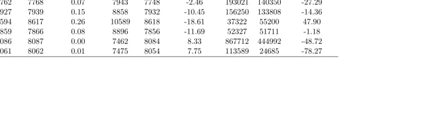
aggre-gate change in trade implied by this experiment for each commodity group is shown in Table 3.15
As we redistribute distance equally across countries, but preserve total distance between all country pairs, trade volumes fall. This reflects the fact that neighbouring countries trade much more with each other than with distant countries, and that the relationship
12In this counterfactual we treat the fixed effects as independent of distance. This treatment differs
from equation (6) where the denominator of the fixed effect term,γi, in equation (6) depends on the sum
of thedij. Moreover the entry and exit of inframarginal firms could change this sum. Our approach is
parsimonious but doesn’t necessarily capture all the possible consequences of changing distance indicated by equation (6). We are grateful to a referee for this point.
13An alternative counterfactual experiment is to also remove the advantage of contiguity. For instance
some countries have many neighbours (for example, Germany has 8 neighbours compared to South Korea that shares a border only with North Korea). The results for this alternative counterfactual experiment are very similar to our main counterfactual experiment (results available on request).
14The general equilibrium effects from these changes, such as impacts on employments or sectoral
output responses and welfare gains, are not the primary issue of concern here. Likewise any general equilibrium effects would be very specific to the specification of the general equilibrium model without adding any particular insight in terms of the relative size of these distortions. For a discussion of the use of general equilibrium models to deal with the endogeneity of country specific prices and multilateral resistance terms in simulations see Anderson and van Wincoop (2003) and Baier and Bergstrand (2009).
15The average trade weighted distance is calculated for the year 2006 using the following formula. Let
J be the set of world markets and J−i be the set of export markets for country i∈J. We define the
average distance to market for country i for commodityc as Di,c =Pjdijsjc, j ∈ J−i, where sjc is
countryj’s share of imports for all countriesj ∈J−i. Likewise the average distance to market implied
by the counterfactual distances isDi,c0 =P
jd¯jsjc, where it will be recalled that ¯djis the counterfactual
between trade and distance is non-linear. In particular Europe consists of many large countries with a lot of trade, while many remote southern hemisphere countries are small. Effectively, by breaking up Europe, we reduce world trade in the counterfactual. Nevertheless There are significant differences by commodity. For example it can be seen that equalizing export distance across countries causes Gas trade to fall by 78% but Iron Ore trade increases by 48%.
[Table 3 about here]
Table 4 summarizes the actual and counterfactual exports share by broad region.
[Table 4 about here]
4.1
Food and Raw Materials
From Table 1 we saw that Europe and Central Asia alone accounted for over 50% of world Food imports with the two other major regions, East Asia and North America, having, respectively, 16% and 19%. Thus European and Central Asian countries have a clear advantage when it comes to Food exports. In our experiment, European and Central Asian countries lose their world share of Food exports, which falls from 48% to 25%, a 23 percentage point loss in market share (Table 4). Most other regions gain exports share but particularly Latin America, and Australia and New Zealand. The pattern for Raw Materials is similar, with Europe and Central Asia appearing to have the largest location advantage and Latin America being the most disadvantaged region. The main difference is that East Asia and South Asia also lose market share in this case.
4.2
Minerals
From Table 1 and the preceding discussion we saw that that Minerals imports are focused geographically on East Asia, particularly China, Japan and South Korea. It can be seen from Table 4 that Australia and New Zealand and the Americas (specifically, Brazil, Chile, Canada and the USA) dominate the world supply of Minerals, accounting for 48% of world Minerals exports.
(South Africa) – a roughly neutral impact in North America and a collapse of exports in Europe-Central Asia and East Asia. The combined share of Australia and New Zealand and Latin America increases by twenty percentage points from just over 30% to just over 50% of world Minerals trade.
Hence in the world Minerals market there is a relatively large dispersion between pro-ducers and their main destination markets and this dispersion has a very significant cost on the southern Minerals giants such as Australia and Brazil. This also suggests that these regions still stand to make substantial gains in terms of world market shares in the event of new transport technologies and reductions in transport costs.
4.3
Iron Ore
Iron Ore is a subset of Minerals that, as noted above, is mainly imported by East Asia, especially China. It is dominated on the supply side by Brazil and Australia, which mutually account for 61% of world exports. Because of this concentration of demand in East Asia, Brazil is much farther from the world’s largest Iron Ore importers than Australia. So in relative terms Australia is close to the Iron Ore market.16
In the counterfactual Australia’s market share falls by approximately one third to 23% of world trade. Likewise European based exporters such as Sweden and Ukraine are driven out from the market. Brazil however almost doubles its export share from 31% to 59% of world exports. Similar results are found for the other Latin American countries – Peru, Venezuela and Chile – though their shares of world trade are very small. Thus, as shown in Table 4, the Latin American share increases from 34% to 65% of world exports. Moreover total Iron Ore trade flows increase in the counterfactual, suggesting that Brazil’s distance from China is an important impediment to world Iron Ore trade.
The large changes in world Iron Ore trade shares reflect not only Brazil’s relatively large distance from its market, and Australia’s proximity to China, but also the very large elasticity of Iron Ore trade with respect to distance of -1.96. The experiments thus support the popular view that Australia has benefited from its locational advantage to China in the Iron Ore market.
16In absolute terms the Iron Ore market is the most dispersed with trade weighed distance falling by
4.4
Coal
Whereas the world Coal market is relatively dispersed across northern hemisphere coun-tries in Europe-Central Asia and East Asia, Table 4 shows that supply is very concen-trated in the South. Australia and New Zealand account for 28% of the world exports. Removing any distance disadvantage increases their share of world exports substantially to 47%.
Hence with respect to Coal the popular notion that Australian resource exports have benefited from its proximity to Asia can be seen in a somewhat different light. For Coal, Australia’s relative proximity to Japan and China does not offset the cost of remoteness from Europe. Moreover, unlike Iron Ore, there are apparently no major Latin Amer-ican suppliers that would be in a position to expand substantially supply if distance disadvantages were removed.
The results also show that South Africa faces a similar geographical disadvantage as Australia - though its Coal exports are substantially smaller. The two second largest exporters, however, China and Russia, have significant geographical advantages being relatively close to both East Asian and European-Central Asian markets.
4.5
Petroleum
Comparing Tables 1 and 4 it can be seen that the demand for imported Petroleum is almost equally split between Europe-Central Asia (36%), North America (25%) and East Asia (29%) while the supply of Petroleum is essentially split equally between the Middle-East (32%) and Europe-Central Asia, including Russia, (34%).
4.6
Gas
The Gas market lacks the South-North pattern seen in the preceding commodity mar-kets due to significant Gas exporters in the northern hemisphere. The exception is the Australia-Indonesia-Malaysia East Asia LNG corridor which accounts for 17% of world Gas exports.
Central to the Gas market is the issue of the delivery mode. Over a short distance pipelines are the cheapest mode of transport, while over long distances, shipping liquefied gas (LNG) is the only viable solution. Indeed, estimating the model separately for LNG and for Gaseous gas, we find that the elasticity of distance for Gaseous Gas (-5.7) is approximately double the LNG elasticity (-2.7) (Table 5).17 In either case however the elasticity of trade to distance is much higher than for other commodities.
Thus countries that ‘share a border’ with a large Gas importer benefit significantly from their geographical location, with notably Canada and the USA market and, to a smaller extent, Algeria and the European market. At the other extreme the Middle-Eastern countries, in particular Saudi Arabia and Qatar, but also Australia, suffer from the infeasibility of being connected via pipelines to large import markets. These countries also account for a large fraction of the total world trade in gas. Consequently, when we equalize distance in the counterfactual, the total Gas trade volumes collapse, as was shown in Table 3.
In relative terms however counterfactual leads to major changes in the Gas market, with current big players, such as Canada and Algeria, being almost completely eliminated from the market and large LNG exporters such as Australia, Saudi Arabia and Qatar, substantially increasing their world shares. The changing regional shares can be seen in Table 4. These relative changes are of interest given that there have been recent technological advances that have lowered the cost of transporting LNG (Ruester 2010).
[Table 5 about here]
17To maximise the sample size and to ensure that as many major natural resource exporters are
5
The Tyranny of Distance
Given the preceding discussion it is clear that a country’s location has an important effect on its volume of resource trade. Brazil exports much more Petroleum and much less Minerals than it would if it were located elsewhere. Australia is close to Asia and this is typically regarded as being very advantageous in terms of resource exports. We have found that this is true for Iron Ore but Australia still suffers a tyranny of distance in terms of Coal.
How then do these costs and benefits of location add up for each country and how can we compare these costs across countries? Figure 1 shows the percentage change in total resource exports for each country. The overall picture is dramatic – showing a stark north-south divide. The countries at the greatest disadvantage are the antipodean countries: Australia, New Zealand and the South American and South African resource exporters. There are some interesting exceptions however, with for example, Chile being much more disadvantaged relative to Argentina. The locational advantage of Canada, Mexico, and Algeria are also highlighted. For Mexico this entirely due to its Petroleum sector while for Canada the key sectors are both Petroleum and Gas.
Likewise other example of the least remote countries are the Slovak Republic, Algeria, Norway and Mexico which have a particular advantage of being oil exporters with a close proximity to large markets. The “benevolence of proximity” adds around 30-50% to their Petroleum export sales relative to an average country. There are also clear large locational gains from being inside Europe, with these mostly reflecting trade in Food. Similarly Poland and the Czech Republic benefit considerably from having coal deposits within Europe.
For the most geographically disadvantaged countries the losses are very significant, ex-ceeding 30%. Chile and New Zealand are particularly affected with a loss of around 50%. For example this implies Chile’s and New Zealand’s resources trade flows would be around 50% larger if their distance to exports markets were at the world average for each commodity.18
The reasons behind these changes differ by country. For New Zealand the key factor
18These values are all percentage changes. In terms of absolute changes the countries that stand the
is its distance from European Food markets. For Chile and Brazil the distance from world Minerals demand is the key component. As we have seen above this is due to their distance from Asia relative to other countries. Likewise Australia and South Africa have a very similar pattern in terms of the composition of their distance disadvantage in Food, Minerals and Coal. As noted Argentina is not as remote overall as, for example, Chile and Brazil, because it exports Petroleum and Gas to North America, and because minerals are a relative small component of its exports. Hence it is not affected by the distance to Asia in the same way Brazil is.
[Figure 1 about here]
5.1
Ad Valorem
Tax Equivalents
A useful way to interpret these trade volume measures is to consider what they might imply in terms of an export destination country tariff equivalent. In our model the export trade flows are modelled as being determined by firms facing increasing marginal costs and exogenous world prices. In this setting the demand elasticity is infinite and the elasticity of supply determines the responsiveness of export volumes to price changes. Thus, for example industry studies of iron ore supply assume short to medium term supply elasticities of 0.5 (Fishera, Beare, Matysek and Fisher 2015). Hence, in this case, a 10% increase in export quantities can be thought of as equivalent to a 20% export tax.
Information about supply elasticities for resource sectors more generally is very scant. Nevertheless the limited studies that exist suggest that the elasticities of resource supply are generally equal to or less than unity. This implies therefore that the large predicted changes in quantities will imply similar, if not larger,ad valorem tariff equivalents.
Likewise trade volume measures can also be converted to approximate welfare cost mea-sures for a broad class of models using just a few key parameter values that are read-ily available (Arkolakis, Costinot and Rodr´ıguez-Clare 2012, Costinot and Rodriguez-Clare 2013).19 Specifically Arkolakis et al. (2012) show that the change in consumption,
C toC0, is given by the expressionC0/C = (λ0/λ)1/η, whereλis the share of domestically produced consumption and η is the elasticity of imports with respect to relative import prices.20
19These are models with CES preferences such as Dixit-Stigliz monopolistic competition models and
Armington models or Ricardian models following Eaton and Kortum (2002).
20Technically this expression also assumes that output is a linear function of endowments. As with
We can use this expression to infer the approximate magnitude of the welfare gains from the change in trade volumes, using our predicted changes in resources exports and data on the resource share of exports; the consumption share of imports, and an assumed trade elasticity η of 5 based on Arkolakis et al. (2012).21 For Australia, for example,
we find that the 34% increase in resource exports translates into a 24% increase in total exports. Given an import to GDP share of 0.21, and η = 5, this implies a welfare gain of 1.3%. We obtain very similar values for South Africa and New Zealand. For some resource exporting counties with very large import shares, however, the welfare gains are much higher. For example we find a welfare gain of 2.6% for Chile, 2.3% for Paraguay and Paraguay and 4.1% for Guyana. These are quite large gains in the context of the literature.
Thus we find that location matters considerably in the resource sector both in terms of tariff volumes, tariff equivalents and welfare implications. The countries most affected are the southern resource exporting countries, particularly Australia, New Zealand, South Africa and some of the South American countries, Brazil Chile and Uruguay. For these countries, the costs of distance are quite large compared to an average country and imply significant welfare costs.
6
Conclusion
While a broad literature exists on the importance of geography in explaining the volume of trade across countries, little is known about the importance of distance in explaining the predominance of some countries in resource exports. In contrast to manufacturing trade we have find that location plays a very important role in explaining trade in resource commodities. This is due to both the relatively high transports costs and the fact that resource export supply is limited by natural endowments.
We show, first, that many resources – but particularly Iron-Ore and Gas – have very large elasticities of trade with respect to distance. However the impact of distance also depends the geographic separation of the export sources and the geographic distribution of demand. Thus we also show that equalizing distances to markets would have large
21This implicitly assumes a demand side specification for the exporting country. For example we can
effects in some markets and on a country share of world resource exports.
In particular we found that the southern resource exporting countries, particularly Chile, South Africa, Brazil, Australia and Peru are significantly disadvantaged by their location. Likewise New Zealand was also found to have a large disadvantage due to its exports of Food. Despite their southern hemisphere location, however, South American petroleum exporters were found to have a smaller total disadvantage, however, due to their proximity to the USA. The costs to these countries turn out to be equivalent to very large tariffs on their key export sectors, that may be in the range of 10-50 percent, and so also imply significant welfare costs.
Consequently, we conclude that the ability of many countries to be competitive in the world resource markets depends a great deal on their location and endowments. This suggests that the responsiveness of extraction firms to national policies, for example with respect to resource taxation and regulation, may be quite low, particularly in Europe.
For example resource taxes have featured heavily in recent Australian state and federal elections, where resource lobby groups argued that taxes on the resource sector will cause multinational countries offshore. There has been very little evidence on the credibility of this threat. Our results lend support to the view that Australia has benefited from its locational advantage to China and that the major competitor, Brazil, faces a significant cost disadvantage in the Iron Ore market due to its location.
Appendix A: Definition of Variables
Table 1: Regional Share of World Imports in 2006
Europe and North America South America Middle-East East Asia Australia South Asia Sub-Saharan
Central Asia and NZ Africa
All 44.23 21.78 5.57 2.51 21.80 1.47 1.56 1.09
Food 52.96 16.15 5.42 4.65 17.54 1.27 0.58 1.44
Raw 41.92 13.61 5.25 3.10 31.18 0.78 3.02 1.16
Min. 38.30 6.72 3.52 1.12 45.99 0.31 3.76 0.28
Iron Ore 22.51 2.89 2.35 1.03 70.53 0.38 0.20 0.11
Coal 40.62 6.83 5.03 2.14 37.27 0.11 7.44 0.55
Petrol 35.88 25.33 3.61 1.48 27.57 1.64 3.21 1.27
Gas 34.57 26.85 5.64 1.96 28.91 0.16 1.81 0.11
Table 2: PPML Results
(1) (2) (3) (4) (5) (6) (7)
Food Raw Min. Iron Ore Coal Petrol Gas
ln gdp 0.479*** 0.458** -0.406* -0.008 0.792** 0.904*** 0.212
(0.136) (0.204) (0.242) (0.759) (0.328) (0.200) (0.818)
p ln gdp 0.803*** 1.553*** 2.384*** 3.032*** 1.089*** 1.006*** -0.240
(0.150) (0.223) (0.240) (0.295) (0.394) (0.309) (0.741)
ln pop -1.274*** -1.214*** 2.109*** 2.117 0.115 -0.925*** 1.029
(0.334) (0.454) (0.749) (1.911) (1.570) (0.296) (0.715)
p ln pop -0.126 -0.863* -1.714** -1.754 0.176 0.926 6.935**
(0.329) (0.497) (0.744) (1.125) (1.020) (0.829) (3.020)
ln distwces -0.968*** -0.864*** -0.959*** -1.964*** -1.220*** -1.372*** -2.557***
(0.033) (0.037) (0.062) (0.197) (0.127) (0.069) (0.191)
ln land paire -0.027 -0.141** 0.043 -0.135 0.082 0.095 0.110
(0.055) (0.059) (0.085) (0.239) (0.248) (0.113) (0.180)
landlocked 1 -0.410 3.827* 8.455*** 8.069* 2.707 3.806 9.772
(1.634) (2.210) (3.135) (4.374) (4.565) (3.345) (7.663)
landlocked 2 -0.177 8.302* 17.431*** 15.189* 7.225 9.652 19.490
(3.283) (4.435) (6.265) (8.701) (9.155) (6.686) (15.371)
contig 0.248*** 0.358*** 0.590*** 0.839** 0.361 0.158 0.596*
(0.090) (0.088) (0.130) (0.337) (0.244) (0.168) (0.305)
island 1 -0.378 0.437 3.789 8.866 1.848 6.708 25.882*
(1.913) (2.802) (4.325) (6.356) (5.980) (4.529) (13.664)
island 2 -0.558 0.790 7.965 17.876 4.215 13.254 52.465*
(3.764) (5.556) (8.666) (12.698) (11.900) (9.120) (27.299)
comlang ethno 0.362*** 0.115 0.236* 0.169 0.006 0.549*** -0.087
(0.111) (0.111) (0.123) (0.287) (0.220) (0.188) (0.268)
colony 0.179 0.101 0.411*** 1.734*** 0.382* 0.228 0.419
(0.123) (0.128) (0.145) (0.330) (0.213) (0.195) (0.327)
hum k 0.177*** 0.096* 0.041 0.203 0.189* 0.029 0.350
(0.035) (0.056) (0.055) (0.198) (0.111) (0.079) (0.314)
p hum k 0.015 0.068 0.180*** -0.016 0.004 -0.038 -0.117
(0.021) (0.058) (0.046) (0.085) (0.107) (0.047) (0.139)
Constant 12.670*** 9.568** -8.123 -12.152 -5.694 0.747 -19.702
(2.859) (4.856) (6.286) (17.392) (13.509) (4.926) (15.879) Observations 74,984 74,984 74,984 74,984 74,984 74,984 74,984
Pseudo R2 0.908 0.897 0.870 0.932 0.892 0.859 0.902
Table 3: Distance and Total Trade
Unweighted Distance Weighted Distance Trade Value
Actual Count. Change in % Actual Count. Change in % Actual Count. Change in %
Food 7374 7381 0.09 7216 7385 2.34 493876 310746 -37.08
Raw 7762 7768 0.07 7943 7748 -2.46 193021 140350 -27.29
Min. 7927 7939 0.15 8858 7932 -10.45 156250 133808 -14.36
Iron Ore 8594 8617 0.26 10589 8618 -18.61 37322 55200 47.90
Coal 7859 7866 0.08 8896 7856 -11.69 52327 51711 -1.18
Petrol 8086 8087 0.00 7462 8084 8.33 867712 444992 -48.72
Table 4: Regional Share of World Exports in 2006: Actual and Counterfactual
Europe and North America Latin America Middle-East East Asia Australia South Asia Sub-Saharan
Central Asia and NZ Africa
Panel A: Actual
Food 47.82 15.50 14.48 1.45 11.89 4.78 1.67 2.41
Raw 35.25 25.90 11.00 1.12 19.19 4.09 1.06 2.39
Min. 29.15 15.18 19.77 3.19 11.88 12.64 3.63 4.57
Iron Ore 10.55 6.17 34.41 0.29 1.76 30.12 12.57 4.13
Coal 20.11 13.52 6.49 0.22 23.33 28.09 0.02 8.22
Petrol 34.07 6.39 12.91 32.06 11.50 0.97 0.67 1.43
Gas 24.86 27.70 4.63 24.99 14.59 3.19 0.01 0.04
Europe and North America Latin America Middle-East East Asia Australia South Asia Sub-Saharan
Central Asia and NZ Africa
Panel B: Counterfactual
Food 25.24 19.03 24.94 1.24 12.33 10.87 2.19 4.16
Raw 19.91 29.68 19.92 0.90 17.57 7.60 1.00 3.41
Min. 12.70 15.41 35.08 2.25 7.15 17.87 2.64 6.89
Iron Ore 0.99 3.26 65.04 0.06 0.18 22.91 2.26 5.31
Coal 5.69 12.21 8.20 0.08 14.25 47.25 0.01 12.30
Petrol 25.15 3.48 12.42 45.74 7.05 2.40 0.92 2.85
Gas 13.42 4.86 6.81 41.10 20.75 12.76 0.01 0.29
Europe and North America Latin America Middle-East East Asia Australia South Asia Sub-Saharan
Central Asia and NZ Africa
Panel B: Change
Food -22.58 3.53 10.46 -0.21 0.44 6.09 0.52 1.76
Raw -15.35 3.78 8.92 -0.22 -1.62 3.52 -0.06 1.02
Min. -16.45 0.23 15.32 -0.94 -4.72 5.24 -0.99 2.33
Iron Ore -9.56 -2.92 30.63 -0.22 -1.58 -7.21 -10.31 1.18
Table 5: PPML Results: Natural Gas
(1) (2) (3) (4) (5) (6)
Nat. Gas LNG Gaseous Nat. Gas LNG Gaseous
ln gdp 0.184 1.331 -3.303 -0.100 0.764 -2.145
(1.151) (1.120) (2.326) (1.110) (0.895) (2.000)
p ln gdp 0.390 1.774 0.126 0.688 -0.160 -0.137
(1.343) (1.459) (2.289) (1.406) (1.764) (2.196)
ln pop 0.836 -0.052 -3.576 0.711 -0.263 -3.133
(0.893) (0.810) (7.835) (0.881) (0.681) -7.434 p ln pop 8.388** 11.381* 4.609 9.210* 29.756*** 5.187
(4.168) (6.800) (6.281) (4.927) (10.100) (6.422) ln distwces -3.713*** -2.672*** -5.674*** -3.696*** -3.185*** -5.583***
(0.416) (0.372) (0.851) (0.428) (0.470) (0.870)
ln land paire 0.110 -0.332 0.324 0.109 -0.329 0.329
(0.283) (0.249) (0.662) (0.283) (0.248) (0.665) landlocked 1 11.216** 16.958*** 10.298 12.826** 34.200*** 9.856
(4.501) (5.642) (8.506) (6.168) (10.793) (8.224) landlocked 2 22.200** 39.743*** 19.519 25.417** 74.251*** 18.631
(9.109) (11.240) (17.093) (12.429) (21.462) (16.535)
contig 0.780 0.709 -0.708 0.779 0.605 -0.699
(0.541) (1.371) (0.557) (0.540) (1.266) (0.559) island 1 27.179** 38.293* 18.686 30.586** 96.711*** 19.781
(11.947) (19.592) (17.934) (15.347) (33.520) (18.384) island 2 55.000** 76.787** 42.731 61.813** 193.615*** 44.877
(23.878) (39.163) (35.723) (30.717) (67.028) (36.557)
comlang ethno 0.145 -0.312 0.545 0.144 -0.351 0.540
(0.462) (0.478) (0.779) (0.461) (0.476) (0.780)
colony 0.558 1.471* -0.912 0.555 1.399* -0.902
(0.476) (0.883) (0.728) (0.476) (0.833) (0.731)
hum k 0.291 -0.318 0.029 0.342 0.218 0.056
(0.387) (0.324) (0.355) (0.414) (0.427) (0.412)
p hum k -0.057 -0.654 0.091 -0.072 -0.046 0.037
(0.170) (0.448) (0.170) (0.178) (0.563) (0.201)
dist y2000 0.030 0.137 0.043
(0.055) (0.112) (0.135)
dist y2001 -0.143 0.129 -0.115
(0.095) (0.141) (0.199)
dist y2002 -0.095 0.201 -0.029
(0.088) (0.153) (0.234)
dist y2003 -0.033 0.288 0.114
(0.121) (0.186) (0.283)
dist y2006 0.064 0.849** -0.310
(0.225) (0.336) (0.520) Constant -17.494 -35.570* 15.873 -20.707 -97.939*** 15.237
(13.995) (21.157) (21.932) (18.087) (34.016) (21.054) Observations 52,876 52,876 52,876 52,876 52,876 52,876
Table A.1: Variables’ Definition
Variable Definition Source
Dependent Variables
Food SITC-1: 00-09 and 11-12. COMTRADE/WITS
Raw SITC-1: 21-26, 29 and 41-43. COMTRADE/WITS
Minerals SITC-1: 27-28. COMTRADE/WITS
Iron Ore SITC-1: 281. COMTRADE/WITS
Coal SITC-1: 32. COMTRADE/WITS
Petrol SITC-1: 33. COMTRADE/WITS
Gas SITC-1: 34. COMTRADE/WITS
Nat. Gas SITC-3: 343. COMTRADE/WITS
LNG SITC-3: 3431. COMTRADE/WITS
Gaseous SITC-3: 3432. COMTRADE/WITS
Independent Variables
ln gdp and p ln gdp Log of GDP. WDI
ln pop and p ln pop Log of population (in millions). WDI
ln land paire Log of total land area of country pair. WDI
ln distwces Weighted great-circle distance (based on population distribution) between country pair. CEPII
landlocked 1 1: 1 country in the country pair is landlocked, 0 otherwise. CEPII
landlocked 2 1: 2 countries in the country pair are landlocked, 0 otherwise. CEPII
contig 1: countries are continguous, 0 otherwise. CEPII
island 1 1: 1 country in the country pair is an island, 0 otherwise. CEPII
island 2 1: 2 countries in the country pair are islands, 0 otherwise. CEPII
comlang ethno 1: a language is spoken by at least 9% of the population in both countries, 0: otherwise. CEPII
colony 1: country pair has ever been in a colonial relationship, 0: otherwise. CEPII
hum k and p hum k Exponent of 0.15 times the average years of schooling among the 25+ years old. Barro and Lee (2010)
References
Allen, Treb (2014) ‘Information frictions in trade.’ Econometrica 82(6), 2041–2083
Anderson, James E., and Eric van Wincoop (2003) ‘Gravity with gravitas: A solution to the border puzzle.’ The American Economic Review 93(1), 170–192
Arkolakis, Costas, Arnaud Costinot, and Andr´es Rodr´ıguez-Clare (2012) ‘New trade models, same old gains?’ The American Economic Review 102(1), 94–130
Athukorala, Prema-Chandra (2009) ‘The rise of China and East Asian export perfor-mance: Is the crowding-out fear warranted?’ World Economy 32(2), 234–266
Baier, Scott L, and Jeffrey H Bergstrand (2009) ‘Bonus vetus OLS: A simple method for approximating international trade-cost effects using the gravity equation.’ Journal of International Economics 77(1), 77–85
Barro, Robert, and Jong-Wha Lee (2010) ‘A new data set of educational attainment in the world, 1950-2010.’ NBER Working Paper 15902
Behrens, Kristian, Carl Gaign´e, Gianmarco IP Ottaviano, and Jacques-Fran¸cois Thisse (2006) ‘Is remoteness a locational disadvantage?’ Journal of Economic Geography 6(3), 347–368
Blainey, Geoffrey (2001)The tyranny of distance: How distance shaped Australia’s history (Australia: Pan Macmillan)
Boulhol, Herv´e, and Alain De Serres (2010) ‘Have developed countries escaped the curse of distance?’ Journal of Economic Geography10(1), 113–139
Chor, Davin (2010) ‘Unpacking sources of comparative advantage: A quantitative ap-proach.’ Journal of International Economics82(2), 152–167
Costinot, Arnaud, and Andres Rodriguez-Clare (2013) ‘Trade theory with numbers: Quantifying the consequences of globalization.’ NBER Working Papers 18896
Deardorff, Alan V. (1995) ‘Determinants of bilateral trade: Does gravity work in a neo-classical world?’ NBER Working Paper 5377
Disdier, Anne-Celia, and Keith Head (2008) ‘The puzzling persistence of the distance effect on bilateral trade.’ Review of Economics and Statistics90(1), 37–48
Fishera, Brian S., Stephen Beare, Anna L. Matysek, and Anna M. Fisher (2015) ‘The impacts of potential iron ore supply restrictions on producer country welfare.’ Tech-nical Report, BAEconomics
Frankel, Jeffrey A. (1997) Regional trading blocs in the world economic system (Wash-ington: Institute for International Economics)
Greenaway, David, Aruneema Mahabir, and Chris Milner (2008) ‘Has China displaced other Asian countries’ exports?’ China Economic Review19(2), 152–169
Head, Keith, and Thierry Mayer (2013) ‘What separates us? Sources of resistance to globalization.’ Canadian Journal of Economics/Revue Canadienne d’ ´Economique 46(4), 1196–1231
(2014) ‘Gravity equations: Workhorse, toolkit, and cookbook.’ In Handbook of In-ternational Economics, ed. Gita Gopinath, Elhanan Helpman, and Kenneth Rogoff (Amsterdam: Elservier) pp. 131–195
Helpman, Elhanan, Marc Melitz, and Yona Rubinstein (2008) ‘Estimating trade flows: Trading partners and trading volumes.’ The Quarterly Journal of Economics 123(2), 441–487
Kalnins, Arturs, and Francine Lafontaine (2013) ‘Too far away? the effect of distance to headquarters on business establishment performance.’American Economic Journal: Microeconomics 5(3), 157–179
Levchenko, Andrei A (2007) ‘Institutional quality and international trade.’ The Review of Economic Studies 74(3), 791–819
Linders, Gert-Jan M., and Henri L.F. de Groot (2006) ‘Estimation of the gravity equation in the presence of zero flow.’ Tinbergen Institute Discussion Paper 06-072/3
OECD (2011) ‘Clarifying trade costs in maritime transports.’ OECD Trade Committee [On line] http://www.oecd.org/trade/its/44387935.pdf (accessed on the 22-08-16).
Overman, Henry G, Stephen Redding, and Anthony Venables (2003)The economic geog-raphy of trade, production and income: A survey of empirics (Blackwell Publishing)
Romalis, John (2004) ‘Factor proportions and the structure of commodity trade.’ The American Economic Review 94(1), 67–97
Santos Silva, Joao M. C., and Silvana Tenreyro (2006) ‘The log of gravity.’ Review of Economics and Statistics 88(4), 641–658