Application of high speed filming techniques to the study of rearwards melt ejection in laser drilling

APPLICATION OF HIGH SPEED FILMING TECHNIQUES TO THE STUDY OF REARWARDS

MELT EJECTION IN LASER DRILLING

ICALEO Conference 2016 - Paper 2309

Connor Jones1, D.B. Hann1, K.T. Voisey1, Scott Aitken2

1_{Faculty of Engineering, The University of Nottingham, Nottingham NG7 2RD, UK.} 2_{AWE, Aldermaston, Reading, RG7 4PR, UK.}

Abstract

Melt ejection is the dominant material removal mechanism in long, ms, pulse laser drilling of metals, a process with applications such as the drilling of cooling holes in turbine blades. Droplets of molten material are ejected through the entrance hole and, after breakthrough, through the exit hole. High speed filming is used to study the ejected material in order to better understand how this debris may interact with material in the immediate vicinity of the drilled hole. Existing studies have quantified various aspects of melt ejection, however they usually focus on ejection through the entrance hole. This work concentrates on rear melt ejection and is relevant to issues such as rear wall impingement. A 2kW IPG 200S fibre laser is used to drill mild steel. High speed filming is combined with image analysis to characterise the rearward-ejected material. Particle size and velocity data is presented as a function of drilling parameters. It is concluded that high speed filming combined with image analysis and proper consideration of process limitations and optimisation strategies can be a powerful tool in understanding resultant debris distributions.

Introduction

Laser drilling is a contactless process that is capable of generating fine holes in traditionally hard to machine materials. Laser drilling encompasses a wide range of lasers, hole sizes, techniques and materials. Several different material removal mechanisms may occur depending on the specific combination of laser parameters and materials used [1]_{. Of interest to this} study, is the laser drilling of holes which are micrometres in diameter, through different metals that measure millimetres in thickness – this is similar to the process which is used to drill cooling holes in turbine blades [2, 3]. These holes are typically drilled using laser pulses with length of the order of milliseconds; where material removal is dominated by melt ejection [2-4]_{. In}

this process, absorption of the laser beam by the top surface of the material generates a melt pool; continued laser irradiation then leads to further heating and vaporization of the surface. The recoil pressure generated by vaporization pushes down on the melt pool. This results in the molten material moving first radially outwards and then upwards before being ejected out of the hole, driven by the combined actions of the recoil pressure and the pressure generated by the assist gas. This melt ejection process allows for a rapid advance of the melt front into the material. The hole depth increases as molten material continues to be generated and driven from ahead of the interaction zone [5]. Efficient melt ejection is important for the quality of the hole. Incomplete ejection of melt results in large heat affected zones and the presence of re-solidified material within the hole, which can lead to cracking [6] as well as introducing hole to hole dimensional variation. As the hole deepens, material is ejected upward, back through the entrance hole. On breakthrough material removal can also occur through the rear, exit, hole. When drilling into a cavity, such as found inside a turbine blade [7]_{, the spread and} adhesion of rear ejected material is of interest.

Observation of characteristics including the extent, direction, timing and droplet size of melt ejection, and how these vary with laser parameters; can provide useful information for process optimisation and further insight into the laser drilling process.

of discrete droplets at 9 – 17 ms-1_{. Obata et al.} [10] _used a combination of modelling and high speed filming with a 210 kHz frame rate to investigate material removal in CO2 drilling of vias in copper on printed wiring boards and determined particle ejection velocities of the order of 1 – 6 ms-1. Okamoto et al. [11] applied 3D particle tracking methods to images gained from two high speed cameras to study the ejection velocity and angle in 0.2 ms Nd:YAG drilling of 150 µm thick stainless steel. For these conditions initial velocities ranging from 75 to 200 ms-1 were observed, with the angle of ejection typically being between 0 and 30⁰ from the work piece surface. No particle size data was reported.

Low et al. [12] _{used various experimental techniques} including high speed filming to study the effect of pulse train modulation on melt ejection. Use of a pulse train, with each pulse increasing in intensity increased the proportion of material ejection through the rear hole.

The combination of high-speed filming and automated image analysis techniques has the potential to collect a vast amount of time resolved numerical data. One aspect of this is the digital particle image velocimetry method which has been successfully applied in a number of fields [13,14]_{. Continuous improvement in the} availability of computing power and user friendly image analysis tools such as Matlab are largely responsible for the expansion of interest in this area.

This work combines the use of high-speed filming and image analysis, demonstrating its use in the study of rear melt ejection in the laser drilling of mild steel.

Experimental Methods

Tests were carried out on a 60 x 60 x 1mm mild steel sheet, using a vertically incident Nd:YAG 2kW IPG fibre laser, λ = 1070 nm. A 200 µm diameter fibre delivered the beam to aYK52 cutting head, with a125 mm collimation length and a 120 mm focal length lens. The laser was focussed on the top surface of the sample, with a 200µm spot size. Nitrogen assist gas supplied co-axially with the laser beam.

High-speed videos were recorded at a range of powers: 500 W, 1000 W, 1250 W, and 1500 W. All work reported here was done using single, 10 ms pulses.

Two image analysis techniques were used; the first method used was streak analysis; the videos for this were taken using an IDT full colour camera that was capable of recording images at 500 fps. However, this was only done with an assist gas of 2bar nitrogen with powers 500W, 1000W, 1250W and 1500W.

The second method used was a particle tracking method. The videos for this were recorded using a Vision Research Phantom V12.1 camera, capable of taking 1280x800 images at 6200fps. A 60mm lens was used with an exposure time of 4µs.

Both cameras were mounted, in the same place, perpendicularly to the laser beam in order to analyse rear ejection, as shown in figure 1. The material and laser were positioned in such a way that no upward ejection could interfere with the rear ejection in the images. The cameras were triggered using an image-based auto trigger. This allowed the cameras to start recording as soon as breakthrough was detected (due to an increase of brightness in the image).

Image Analysis and Processing

Streak Analysis Technique

Both ends of each streak that is fully visible within the frame are then located by manually clicking on them. This produces co-ordinates of the start and end points of each streak. Together with a calibration factor this

Camera

Laser

Sample

Fig. 1 Laser and High-Speed Camera Set-Up

enables the distance moved by each particle to be determined. The calibration factor is simply determined by reference image taken using the same camera set up, graph paper was used for this work. The time the particles moved for is the inverse of the frame rate, this is used to determine the particle velocities.

Particle Tracking Technique

Matlab was used to create a particle tracking program. The first stage is again to crop the images and remove the background by taking a median of all of the images to reduce noise. Six frames are then selected from the video as those that show images in which the particles are separated enough to allow adequate particle tracking, whilst still as close to the point of ejection as possible, to prevent as few as possible from dissapearing off of the screen. For this investigation frames, approximately, 1.6-2.4 ms after the start of ejection were chosen across all videos – these were decided upon using trial and error for validation.

The six frames are converted to binary form, leaving only the particles. A Watershed Transform algorithm [16,17,18] _{is then used as part of a method to segment and}

identify each of the individual particles by recording their centroids (Fig. 3b). Particle diameters are also determined. The recorded centroid values over a chosen number of frames are then imported into a Matlab based particle-tracking program. This program is able to able to use a combination of the Hungarian Linker [15] and commonly used Nearest Neighbour algorithms to approximate tracks over which any particle has moved during the chosen number of frames, which are plotted and displayed within Matlab, as shown in Fig. 3c.

However, the plotted tracks show many particles appear to change direction very suddenly. Examination of the videos confirms that these tracks are erroneous. These erroneous tracks were eliminated automatically. To do this, a straight line algorithm was implemented into the program. Looking at each of the tracks individually, point by point, for the first two centroids, the ‘x’ and ‘y’ co-ordinates are substituted into ‘y = mx +c’, and solved as simultaneous equations to give values for ‘m’ and ‘c’. The value for ‘c’ is then substituted back into the straight line equation for the next centroid, along with its value for ‘y’ and ‘x’, so that a value for the gradient ‘m’ can be calculated. The program can then be edited to allow for a certain variation in gradient which is deemed to be acceptable. This process is repeated for every centroid in the track, and if any do not lie within the gradient varient, then that track is eliminated.

a. Raw frame from high speed camera

b. Frame after background subtraction and conversion to binary form with particle centroids identified by red

crosses.

c. Tracking of centroids through 6 successive frames.

d. Accepted particle tracks.

Fig. 3d shows the accepted tracks, i.e. those that were not eliminated by this process.

Fig. 3 Stages in implementation of particle tracking technique for mild steel drilled with a single 10 ms 500 W

Figure 4 – Central fast jet, seen in 160µs exposure frame from drilling using 1000Wand 2 bar nitrogen assist gas.

Figure 5 – Sections of four successive frames showing exploding particles during 500 W, 2 bar drilling. Once the particles have been tracked, a separate

program is then able to read automatically prerecorded coordinates from the first two programs to output calibrated graphical data for the particle sizes, particle velocities and comparisons of the two. The particle sizes are calculated from the measured particle diameters within the images. The particle velocities are calculated using the distance travelled between subsequent frames in the image, knowing that the time taken between each frame from the frame rate (6200fps).

Results

Direct Observations

There are some obervations that can be made from direct observation of the raw videos without any image analysis. The first is that in each case a considerable amount of rearwards melt ejection is observed with particles being ejected over the full range of 180⁰. It was also observed that for the lower powers, time between laser on time and breakthrough was greater than for the higher powers. The presence of a central fast jet of particles is confirmed (Fig. 4). This had [3] already been identified in streak photography work from 1995. The higher velocity of the central jet compared to the other particles is clear in Fig. 4. Our measurements indicate that particles in this fast jet are travelling at over 30 m s-1_{, whereas the other particles} are moving at approximately 5 m s-1_.

Fig. 6 – Particle velocity results from streak analysis for drilling of mild steel with 2 bar assist gas. In each case the

summed results from 10 individual holes are shown.

Fig. 7 – Particle velocity results from particle tracking for drilling of mild steel with 2 bar assist gas. In each case the

summed results from 50 individual holes are shown. Streak Analysis Results

The streak analysis results are shown in Fig. 6. It can that for each power used there was a distribution of velocities. The measured velocities range up to 14 m s-1_{. Variation in both particle velocity and} particle numbers as a function of power can be seen: there appears to be a greater number of particles for lower powers.

Particle Tracking Results

Fig. 8 – Particle velocity results from particle tracking for drilling of mild steel with 5 bar assist gas. In each

case the summed results from 50 holes are shown. Particle velocity results obtained when a 5 bar assist gas pressure was used are shown in Fig. 8. The same range of velocities are seen, with average velocities being approximately 8 m s-1_{. The number of particles} again appears to decrease with increasing power.

Discussion of Velocity Results

Figs. 6&7 enable comparison of the results obtained by the two different velocity measurement techniques for the same conditions. While it is immediately clear that the results are not identical it is also clear that the results are not inconsistent with each other, if the streak analysis results are considered as a subset of the particle tracking results. The larger number of particles analysed in particle tracking has produced smoother distributions which at first glance may be assumed to be more representative. However, it must be noted that all above comments relate to the number of particles analysed, which is not necessarily the same as the number of particles present.

Comparison of Figs. 3c&d highlights how many particles are eliminated from the analysis process in the particle tracking method: the majority of particle analysed are from the edge of the particle cloud. This may be useful in tracking the evolution of the particle cloud envelope but cannot be regarded as giving a properly representative set of results. The omission of the central region of the distribution is largely due to the particles being too closely clustered together. The resultant overlapping makes it difficult to correctly identify, and therefore track, each individual particle. There is a therefore danger of some systematic self-selection in the particle tracking method as it will only work for particles which remain within the field of view for the selected frames. This e

1AQ1AQ2Z`ZQÀQQ2WWW2222WWWW WWWW2WWWWZSWX2ZQ1QQAis true of the central fast jet where the particles are moving so quickly that they disappear from subsequent frames. These particles are estimated to be moving at velocities of approximately 30 ms-1_{. Similarly the streak analysis} systematically eliminates streaks that do not terminate within the frame, and these are likely to be the longer streaks corresponding to the higher velocity particles.

The smallest particles are also likely to be omitted from the particle tracking analysis. This is not only due to the resolution limit of the camera but also to the thresholding that takes place during the Watershed Transform Function, with particles which are only a few pixels in size being lost.

Overall the streak analysis method typically produce quantified velocities for the majority of particles in the frame whereas particle tracking only does this for 10-30% of the particles detected.

Table 1. Particle analysis summary data Power

(W)

Shots Total number of particles analysed

Particles analysed per shot Streak analysis 2 bar

500 10 828 83

1000 10 851 85

1250 10 167 17

1500 50 1021 20

Particle tracking 2 bar

500 50 1418(11.4%) 28

1000 50 1416(18.7%) 28

1250 50 1104(21.2%) 22

1500 50 276(29.2%) 6

Particle tracking 5 bar

500 50 1854(14.8%) 37

1000 50 1701(14.7%) 34

Fig. 9 – Particle size results for mild steel drilled over a

range of powers with 2 bar assist gas Fig. 10 – Particle size results for mild steel drilled over a

range of powers with 5 bar assist gas

1500 50 596(25.9%) 12

Particle Size Results

The particle tracking method also produces information on particle sizes. Larger numbers of results are presented as these include particles which were eliminated from the velocity measurement due to erroneous particle path identification.

Figs. 9&10 show the particle size results for a range of powers for both 2 and 5 bar drilling. Particles ranging up to 2 mm were seen. For both assist gas pressures, it is clear that the number of particles produced decreases as power increases, confirming the observations made based on the velocity results. For each power used larger numbers of particles are seen for the higher gas pressure. In each case it is clear that the majority of particles are at the low end of the size range, with diameters of less than 500 µm.

Figs. 11&12 replot the low end of the size distributions in order to reveal them in more detail. This confirms that higher particle numbers are seen for each size range for the higher gas pressure for any given power. The shapes of all the particle size distributions for both assist gas pressures are remarkably similar, with a peak in the range of 100 -200 µm. As power increases the number of particles in each size range decreases. This is seen for both gas pressures. It must be noted that there will still be a systematic removal of the smallest particles due to the thresholding process. This may have resulted in the decreased population of the first bin. This will be investigated in future work by particle size analysis of collected ejecta.

500 W

1000 W

1250 W

1500 W

500 W

1000 W

1250 W

Fig. 12 – Particle size results for drilled mild steel with 5 bar assist gas – detail of distribution of smaller particles Fig. 11 – Particle size results for drilled mild steel with 2

bar assist gas – detail of distribution of smaller particles

Further Considerations

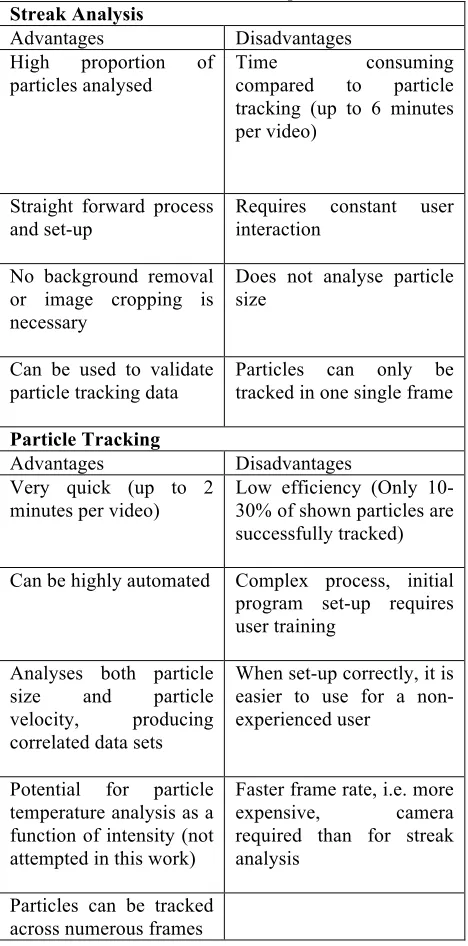
The combination of high speed filming and image analysis has great potential. The results presented here can be used as a case study to highlight factors that need to be considered in such work. The two techniques used here both produced useful results, however each technique has its own limitations which need to be understood before proper interpretation of results can be attempted, key aspects of each process are summarised in Table 2.

Initial examination of high speed videos is required to ensure that sufficient particle separation is achieved. This is a balance between size of field of view and proportion of particles that will be analysed.

The most appropriate technique to use will depend on exactly what results are of interest. A combination of

the two techniques of streak analysis and particle tracking can be beneficial.

It should be noted that any camera capable of a sufficiently high frame rate for the particle tracking method will normally also be able to operate at a lower frame rate suitable for streak analysis, allowing both techniques to be carried out on results from the same camera.

The rearward ejection studied in this work is a 3D phenomenon. This work has used a single viewpoint and therefore only considered two components of motion. 3D consideration can be achieved by using multiple view points, or more simply by checking the symmetry of the process.

Particle-tracking programs and their time dependent analysis could also prove very useful for measuring particle velocities. Of course, the accuracy of such measurements is jeopardised by the 2D nature of

500 W

1000 W

1250 W

1500 W

500 W

1000 W

1250 W

standard high-speed filming set-ups, due to the motion of particles in all planes.

For streak photography, if the time between frames is long compared to the process being studied then the results can be very sensitive to the frame number used. It is recommended that a sensitivity analysis is carried out by analysing a set of different frames to find the optimum.

Table 2. Process comparison

Streak Analysis

Advantages Disadvantages

High proportion of particles analysed

Time consuming

compared to particle tracking (up to 6 minutes per video)

Straight forward process and set-up

Requires constant user interaction

No background removal or image cropping is necessary

Does not analyse particle size

Can be used to validate particle tracking data

Particles can only be tracked in one single frame

Particle Tracking

Advantages Disadvantages

Very quick (up to 2 minutes per video)

Low efficiency (Only 10-30% of shown particles are successfully tracked)

Can be highly automated Complex process, initial program set-up requires user training

Analyses both particle size and particle velocity, producing correlated data sets

When set-up correctly, it is easier to use for a non-experienced user

Potential for particle temperature analysis as a function of intensity (not attempted in this work)

Faster frame rate, i.e. more expensive, camera required than for streak analysis

Particles can be tracked across numerous frames

Conclusions

High speed filming techniques have been successfully applied to extract quantified information on particle sizes and velocities for rearward melt ejection in the laser drilling of mild steel.

Variation in rearward ejection behaviour was noted as a function of power and assist gas pressure.

A number of ejected particles were noted to explode, splitting in several smaller particles during flight after ejection.

Particles were observed to be ejected with a range of velocities for any giving set of laser drilling parameters. Particle velocities of up to 20 m s-1 _were measured, with typical values being approximately 5 m s-1.

The numbers of particles ejected per hole decreased as laser power increased.

Particles with sizes of up to 2 mm in diameter were observed. In each case considered the majority of particles had diameters less than 500 µm.

The particle tracking method can be completely automated however was only able to analyse approximately 20% of the particles present due to particle clustering.

Limitations of the two processes used have been identified and summarised.

Future Work

The techniques presented here will be applied to a wider range of drilling conditions to extend the study of rearwards melt ejection.

References

[1] Schulz, W., U. Eppelt, and R. Poprawe, Review on laser drilling I. Fundamentals, modeling, and simulation. Journal of Laser Applications, 2013. 25(1).

[2] Sezer, H.K., L. Li, M. Schmidt, A.J. Pinkerton, B. Anderson, and P. Williams, Effect of beam angle on HAZ, recast and oxide layer characteristics in laser drilling of TBC nickel superalloys. International Journal of Machine Tools and Manufacture, 2006.

46(15): p. 1972-1982.

[3] French, P.W., D.P. Hand, C. Peters, G.J. Shannon, P. Byrd, and W.M. Steen. Investigation of the Nd:YAG laser percussion drilling process using high speed

filming. in ICALEO'98. 1998. Orlando USA: Laser

Institute of America.

[4] Voisey, K.T., S.S. Kudesia, W.S.O. Rodden, D.P. Hand, J.D.C. Jones, and T.W. Clyne, Melt Ejection During Laser Drilling of Metals. Mat Sci Eng A, 2003.

356: p. 414-424.

[5] Allmen, M.v., Laser Drilling Velocity in Metals. J Appl Phys, 1976. 47: p. 5460-5463.

[6] Poprawe, R., W. Schulz, and R. Schmitt, Hydrodynamics of Material Removal by Melt Expulsion: Perspectives of Laser Cutting and Drilling. Laser Assisted Net Shape Engineering 6, Proceedings of the Lane 2010, Part 1, 2010. 5: p. 1-18.

[7] Kreutz, E.W., L. Trippe, K. Walther, and R. Poprawe, Process Development and Control of Laser Drilled and Shaped Holes in Turbine Components. Journal of Laser Micro Nanoengineering, 2007. 2(2): p. 123-127.

[8] Jetter, V., S. Gutscher, A. Blug, A. Knorz, C. Ahrbeck, J. Nekarda, and D. Carl, Optimizing process time of laser drilling processes in solar cell manufacturing by coaxial camera control. Laser Applications in Microelectronic and Optoelectronic Manufacturing (Lamom) Xix, 2014. 8967.

[9] Yilbas, B. S. Study of liquid and vapor ejection processes during laser drilling of metals Journal of Laser Applications, 7(147).

[10] Sano, Y., M. Obata, T. Kubo, N. Mukai, M. Yoda, K. Masaki, and Y. Ochi, Retardation of crack initiation and growth in austenitic stainless steels by laser peening without protective coating Materials Science and Engineering: A, 2006. 417(1-2): p. 334-340.

[11] Okamoto, Y., H. Yamamoto, A. Okada, K. Shirasaya, and J.T. Kolehmainen, Velocity and Angle of Spatter in Fine Laser Processing. Physics Procedia, 2012. 39: p. 792-799.

[12] Low, D.K.Y., L. Li, and P.J. Byrd, The Influence of Temporal Pulse Train Modulation during Laser Percussion Drilling. Optics & Lasers in Engineering, 2001. 35: p. 149-164.

[13] Scarano, F., Tomographic PIV: principles and practice. Measurement Science & Technology, 2013.

24(1).

[14] White, D.J., W.A. Take, and M.D. Bolton, Soil deformation measurement using particle image velocimetry (PIV) and photogrammetry. Geotechnique, 2003. 53(7): p. 619-631.

[15] Munkres, J, Algorithms for Assignment and Transportation Problems. Journal of the Society for Industrial and Applied Mathematics, 1957, Volume 5, Number 1)

[16] Gonzales, R, Woods, R, Digital Image Processing. Prentice-Hall, 2002

[17] Russ, J, The Image Processing Handbook. CRC Press, 1998

[18] Soille, P, Morphological Image Analysis: