ISSN Online: 2160-0422 ISSN Print: 2160-0414
DOI: 10.4236/acs.2019.94038 Oct. 17, 2019 600 Atmospheric and Climate Sciences
Improving Seasonal Climate Forecasts over
Various Regions of Africa Using the Multimodel
Superensemble Approach
Joseph Nzau Mutemi
Department of Meteorology, University of Nairobi, Nairobi, Kenya
Abstract
Improvements that can be attained in seasonal climate predictions in various parts of Africa using the multimodel supersensemble scheme are presented in this study. The synthetic superensemble (SSE) used follows the approach originally developed at Florida State University (FSU). The technique takes more advantage of the skill in the climate forecast data sets from atmosphere- ocean general circulation models running at many centres worldwide includ-ing the WMO global producinclud-ing centers (GPCs). The module used in this work drew data sets from the Four versions of FSU coupled model system, seven models from the DEMETER project which is the forerun to the current European Ensembles Forecast System, the NCAR Model, and the Predictive Ocean Atmosphere Model for Australia (POAMA), all making a set of 13 in-dividual models. An archive consisting of monthly simulations of precipita-tion was available over all the 5 regions of Africa, namely Eastern, Central, Northern, Southern, and Western Africa. The results showed that the SSE forecast for precipitation carries a higher skill compared to each of the mem-ber models and the ensemble mean. Relative to the ensemble mean (EM), the SSE provides an improvement of 18% in simulation of season cycle of preci-pitation climatology. In Eastern Africa, during December-February season, a north-south gradient of precipitation prevails between Tropical East Africa and the sector of the region towards Southern Africa. This regional scale cli-mate pattern is a direct influence of the Intertropical Convergence Zone (ITZC) across the African continent during this time of the year. The SSE emerges with superior skill scores such as lowest root mean square error above the EM and the member models, for example in the prediction of spa-tial location and precipitation magnitudes that characterize the see-saw pre-cipitation pattern in Eastern Africa. In all parts of Africa, and especially East-ern Africa where seasonal precipitation variability is a frequent cause huge How to cite this paper: Mutemi, J.N.
(2019) Improving Seasonal Climate Fore-casts over Various Regions of Africa Using the Multimodel Superensemble Approach. Atmospheric and Climate Sciences, 9, 600- 625. https://doi.org/10.4236/acs.2019.94038
Received: August 30, 2019 Accepted: October 14, 2019 Published: October 17, 2019
Copyright © 2019 by author(s) and Scientific Research Publishing Inc. This work is licensed under the Creative Commons Attribution International License (CC BY 4.0).
DOI: 10.4236/acs.2019.94038 601 Atmospheric and Climate Sciences human suffering due to droughts and famine, the multimodel superensemble and its subsequent improvements will always provide a forecast that out-weighs the best AtmospheOcean Climate Model. This approach and re-sults herein imply that climate services centres worldwide and Africa in par-ticular can make more objective use of model forecast data sets provided by global producing centres (GPCs) for consensus climate outlooks.
Keywords
Africa, Rainfall, Variability, Prediction, Multimodel, Superensemble, Synthetic, Skill
1. Introduction
The livelihoods and economies of most African countries depend on rain-fed agriculture. The rainfall is seasonal everywhere in the continent and for any given season, there are many periods when the seasonal precipitation amounts are too low to support agriculture and sometimes too heavy. Thus climate ex-tremes in form of droughts and floods are very common in most parts of Africa and they have catastrophic impacts. Improved climate predictions for Africa is the only means of providing quantitative information that can be used for plan-ning and management of socio-economic activities dependent on seasonal pre-cipitation. Good examples are the climatic extremes experienced in East Africa from 1997 through 2000. The period September 1997 to March 1998 was a pro-longed season of devastating rainfall floods in East Africa and those rainfall floods were also associated to the 1997/98 warm ENSO event [1][2]. In Kenya, the 1997/98 floods caused rotting of food crops due to water logging and too much water vapour in the air, submerging of homes in urban and rural areas, huge destruction of roads and bridges and disease outbreaks due to contamina-tion of fresh water supplies. The total economic loss due to the 1997/98 floods over Kenya has been estimated to the tune of US $670 million according to [3]. A severe drought and famine ravaged much of Kenya and Southern Ethiopia from mid 1998 through 2000 and it’s catastrophic impacts included starvation of communities, massive deaths of livestock, lack of water for domestic and indus-trial use including hydropower generation, and closure of industries. The im-pacts of these climatic extremes can be minimized with availability of high accu-racy climate forecasts for Africa, examples of which are illustrated in this study.
DOI: 10.4236/acs.2019.94038 602 Atmospheric and Climate Sciences is not only an interesting scientific venture, but the quantified forecast informa-tion is the only means of providing societies with the quantitative informainforma-tion that can be factored into early warning, policy decision, and disaster prepared-ness in advance of the onset of the extremes. Precipitation in form of rainfall is by far the most important climate element over all the regions of Africa, and it will constitute the main subject of the present study. The objective of this study is to illustrate that it is possible to produce quantitatively skillful seasonal rain-fall/climate forecasts over various regions of the Africa by an optimal combina-tion of real-time forecasts made by the state-of-art global climate models (GCMs) that are running at several centers worldwide. In addition to addressing the fo-recasting needs, accurate predictions can also help in understanding the evolu-tion of the climate mechanisms over the diverse regions of the continent.
One of the most authoritative illustrations of the performance of GCMs in the simulation of various variables of the climate may be found in [6] following the multimodel data sets of the Atmospheric Model Intercomparison Project (AMIP) which has evolved to the World Climate Research Programme (WCRP) Coupled Model Intercomparison Project which is currently at Phase 6 (CMIP6). AMIP results of the late 1990s and the current results from the Atmosphere-Ocean General Circulation Models (AOGCMs) of [7] reveal that there are still big model-to-model differences in simulation of precipitation and this is still the status in climate prediction and projection models “global producing centre models (GPCs)” and CMIP6 models.
Climate forecasts, even from the state-of-the-art AOGCMs inevitably suffer from model differences and model errors. Following the modeling experiences from AMIP results of early 2000s to CMIP5 and CMIP6 results of later 2019, the multimodel ensemble mean (EM) method evolved as one way of overcoming problems associated with model errors (that arise from truncation, discretiza-tion, sampling of boundary conditions, and also from unknown sources). Within the recent years, the use of multimodel forecasts and EM has been an important component in climate predictions done at many centers worldwide [8]. The skill of single and multi-model ensembles has been reported in many studies includ-ing [9][10][11]. Forecasts made from model ensemble systems and the EM still show large space and time variability in skill. Owing to modeling differences, some models have better skill than others, yet the EM weights all the member models equally. The multimodel superensemble scheme developed at the Florida State University (FSUSE) has emerged as an objective means of overcoming these practical difficulties. Some good studies which have used the FSUSE scheme in climate forecasts include [12][13]. By using a criteria that reduces the root mean square error (RMSE) for each individual model forecast based on its past performance, FSUSE product emerges superior to the multi-models and the ensemble mean [14].
fore-DOI: 10.4236/acs.2019.94038 603 Atmospheric and Climate Sciences casts that affect the skill of the consensus product. Poor analysis field and low skill in individual member models degrade the skill [14]. In the conventional approach, the optimal weights used to combine the models are derived from the past performance of each model and minimization of the root mean square er-ror. This criterion however does not ensure that the spatial-temporal multimo-del fields evolve consistently with the dominant spatial-temporal evolution of the observations [15] [16]. Furthermore, redundancy in both multimodel data sets and analysis fields may also mask some useful aspects of the superensemble forecast product. In this study, the conventional superensemble technique is modified by inclusion of these aspects to improve the data quality and enhance the stability of the climate forecasts in the various regions of Africa. This version is called synthetic superensemble, hereafter referred to as SSE. It has given major improvements in seasonal climate forecasts, not only on the improved skill scores, but also predictability of the spatial patterns of the climate evolution and some results on it’s performance may be found in [12][15].
[image:4.595.289.460.516.703.2]A set of 13 GCMs is used in this study to construct the SSE forecasts in five regions of Africa. The sregions are delineated in accordance with the large scale forcing mechanisms that prevail during the course of the year. The regions are presented in Figure 1. In particular, the study attempts to determine if there is an improvement in the use of SSE relative to the EM and individual models in the simulation of annual cycle of precipitation, simulation of the spatial extend and magnitude of seasonal precipitation, and capability in forecasting the sea-sonal extremes, especially those associated with the evolutionary phases ENSO phenomenon. East Africa is used as a region of detailed study. It is a region where, like most tropical areas, interannual variability is strongly influenced by ENSO [17]. The climate models used are discussed in the next section. Section 3 provides an outline of the SSE scheme, the observational analysis fields used, and the measures of skill used. Section 4 is a discussion of results and Section 5 presents conclusions.
DOI: 10.4236/acs.2019.94038 604 Atmospheric and Climate Sciences
2. The Global Climate Models
The first set of climate models used in the study is the FSU ensemble system consisting of four versions the FSU atmospheric model following [18] that is coupled to the Hamburg Ocean Model following [19]. The four FSU versions are configurations of this atmospheric-ocean system with two versions of the cu-mulus parameterization scheme, the modified Kuo scheme following [20], and the Arakawa-Schubert type of scheme following [21]. The model can also use two versions of radiative transfer scheme, an “older” emissivity-absorptivity ra-diative transfer procedure following [22] and a “newer” version of radiative transfer scheme according to [23]. The FSU model with Kuo scheme with ‘older’ radiation is called “KOR”; the version with Kuo scheme combined with “newer” radiation scheme is called “KNR”; the version using Arakawa-Schubert scheme with “older” radiation procedure is “AOR”, and that using Arakawa-Schubert scheme combined with “newer” radiation is called “ANR”.
The fifth model is National Center for Atmospheric Research (NCAR) com-munity climate model (CCM3). CCM3 is spectral and the version used in our study is a triangular truncation at 63 waves, and 26 levels in the vertical (T63L26). A complete description of CCM3 is provided by [24].
The sixth model in the set is the Predictive Ocean Atmosphere Model of Aus-tralia (POAMA). POAMA is also a spectral model, and the version used in these results is a T42L17.
The other seven models in the study are the Development of a European Mul-timodel Ensemble System for seasonal to interannual prediction, called DEMETER multi-model ensemble system. DEMETER prediction system comprised coupled ocean-atmosphere models of the following institutions: the European Centre for Medium-Range Weather Forecasts (ECMWF); UK Met Office (UKMO); Max- Planck Institutfür Meteorologie, Germany (MPI); Istituto Nazionale de Geofisi-ca e VulGeofisi-canologia, Italy (INGV); European Centre for Research and Advanced Training in Scientific Computation, France (CERFACS); Centre National de Recherche Météorologiques, France (CNRM); and Laboratoired’ Océanographie Dynamique et de Climatologie, France (LODYC). DEMETER models have been used in hindcast simulations of monthly global climate over the years 1989-2001, for which initial data assimilation were the ERA-40. The ERA-40 is a European Reanalysis Project that availed high-quality global analysis of atmosphere, land and ocean conditions for the years 1957-2002. The ERA-40 reanalysis are de-scribed in [25]. Details of the DEMETER models and climate simulations may be found in [26]. Table 1 provides an overview of the 13 models and the length of monthly simulations of precipitation for each model used in the study.
3. Data Sets and Methods
3.1. Data Sets
DOI: 10.4236/acs.2019.94038 605 Atmospheric and Climate Sciences Table 1. Summary of the 13 climate models and length of monthly averages of climate parameters available for each model used in the study.
Name and source Model characteristics Length of month by month model forecast data Nature Resolution Initial conditions
KOR, FSU Spectral atmosphere model coupled to HOPE ocean model T63L14 ECMWF with Physical Initialization 1989-2001
KNR, FSU Spectral atmosphere model coupled to HOPE ocean model T63L14 ECMWF with Physical Initialization 1989-2001
AOR, FSU Spectral atmosphere model coupled to HOPE ocean model T63L14 ECMWF with Physical Initialization 1989-2001
ANR, FSU Spectral atmosphere model coupled to HOPE ocean model T63L14 ECMWF with Physical Initialization 1989-2001
CCM3, NCAR Spectral atmosphere model coupled to NCOM Slab ocean model T63L26 AVN 1989-2001
POAMA, AUSTRALIA Spectral atmosphere model coupled to ACOM ocean model T47L17 BAM analysis 1989-2001
CERFACS, FRANCE Spectral atmosphere model coupled to OPA 8.2 ocean model T63L31 ERA-40 1989-2001
CNRM, FRANCE Spectral atmosphere model coupled to OPA 8.0 ocean model T63L31 ERA-40 1989-2001
LODYC, FRANCE Spectral atmosphere model coupled to OPA 8.2 ocean model T95L40 ERA-40 1989-2001
INGV, ITALY Spectral atmosphere model coupled to OPA 8.1 ocean model T42L19 Coupled AMIP-type 1989-2001
MPI, GERMANY Spectral atmosphere model coupled to MPI-OMI ocean model T42L19 Coupled Run 1989-2001
UKMO, UK Spectral atmosphere model coupled to GloSea OGCM ocean model T63L31 ERA-40 1989-2001
ECMWF, Europe Spectral atmosphere model coupled to HOPE-E ocean model T95L40 ERA-40 1989-2001
(CPC) precipitation called CMAP. The data is global, starting from 1979 to present and the part used in the study was for the 13 years 1989-2001. CMAP data is created by a technique that produces monthly values and patterns of global precipitation by merging rain gauge observations with precipitation esti-mates from several satellite-based algorithms that makes use of infrared and mi-crowave channels. CMAP data set may contain an artificial downward trend for the period after 1996. In the study, the data is used for qualitative applications and results are verified against station records wherever applicable. A descrip-tion of CMAP data is according to [27].
DOI: 10.4236/acs.2019.94038 606 Atmospheric and Climate Sciences were extracted and studied using the multimodel superensemble scheme as out-lined in the next section.
3.2. The Multimodel Superensemble Scheme
The Florida State University multimodel superensemble technique has been de-veloped as a tool for making skillfully deterministic forecasts by a combination of global model forecasts that are made by many centers round the world. The scheme follows the studies of [8][12][28] briefly outlined as follows. Given a set of climate forecasts from a group of “N” multilevel global models, the conven-tional multimodel superensemble (S) is defined by the multiple linear regression equation:
(
)
1 N
i i i
i
S a Y Y Z
=
=
∑
− + (1)where S is the multimodel superensemble, ai is a statistical weight for the ith model, Yi is the ith model forecast, Yi is time average of the forecast by the ith
member model, and Z is the time average of the observation. For the deter-mination of the statistical weights, the forecast time line is split into 2 parts, a training period and a validation period. The statistical weights are then deter-mined by the minimization of the root-mean-square error (RMSE) function (E):
(
)
21 rain T
t t
t
E S Z
=
=
∑
− (2)where Train denotes the length of the training period. St is the multimodel supe-rensemble and Zt the observation. This process is also referred to as the conven-tional multimodel superensemble scheme and the regression coefficients ai are solved for using a Gauss-Jordan elimination algorithm. The weights are calcu-lated at every grid point and at every vertical level over the whole training period of the superensemble. For a single level climate parameter such as precipitation, there are as many as 1.7 × 10⁶ weights.
For all the models, the total length of monthly data was 13 years and 12 months for each year. This length was too short to give stable results in forecasts of climate. Cross validation was used to increase the statistical stability the cli-mate forecasts. A good discussions on the usefulness of cross validation may be found in [29][30]. The cross validation procedure was done by exclusion of one year at a time, training the superensemble with the remaining data series and using the weights obtained to forecast the year excluded. All the climate results discussed in this study are cross validated.
3.3. The Multimodel Synthetic Superensemble Scheme
DOI: 10.4236/acs.2019.94038 607 Atmospheric and Climate Sciences The multimodel predictor data set for each model and the predict and analysis field are first pre-processed into empirical orthogonal functions (EOFs) that represent the most significant modes of internal variance in space and the cor-responding principal components (PCs) that track the temporal evolution of the map patterns. Assuming that there are a total of “m” leading EOFs and PCs of each member model “i” and observations, all of which are determined over a training length (t), the predictand (Z) and the multimodel predictor set (Yi) are expressed as linear combinations of EOFs and PCs by:
( )
( ) ( )
1
, M m m
m
Z x t Z t e x
=
=
∑
(3)( )
,( ) ( )
, 1, M
i i m i m
m
Y x t Y t e x
=
=
∑
(4)where Z tm
( )
, Yi m,( )
t and ei m,( )
x are the PC and EOF corresponding to themth mode for the observation and the ith member model. M is the total number of EOFs used. The number of EOFs used in the analysis is such that the cumula-tive variance recovered by those EOFs is at least 95% because the objeccumula-tive of using EOFs in this case is to improve the quality of the data sets. The PCs re-quired in Equations (3) and (4) are calculated over the length of training phase (t).
The next problem is the determination of spatial patterns of multimodel pre-dictor field that evolves in a way that is most consistent with the EOFs of ob-served analysis. This consistent pattern is obtained by a regression of the predic-tand PCs calculated by Equation (3) onto the PCs of the models calculated by Equation (4). This is a linear regression problem on EOF space and it is given by the equation:
( )
, ,( )
,( )
1 M
i m i m i m
m
Z t a Y t r t
=
=
∑
+(5)
where ai,m are regression coefficients and ri,m is the residual error of the ith model at the mth EOF mode. The coefficients a
i,m are determined such that the residual error variance E(r2) is minimum and once the coefficients are determined, PCs of the predictor multimodel set over the total time line (T) are given the equa-tion:
( )
, ,( )
1 M reg
i i m i m
m
Y T a Y T
=
=
∑
(6)
The new PCs are computed for each model, and they are referred to as mul-timodel synthetic ensemble predictor set. The synthetic mulmul-timodel predictor field is given by:
( )
,( ) ( )
1
, i m
M
syn reg
i m
m
Y x T Y T e x
=
=
∑
(7)DOI: 10.4236/acs.2019.94038 608 Atmospheric and Climate Sciences
3.4. The Statistical Measures of Skill
The measures of skill used in the study include the root mean square error (RMSE) and anomaly correlation. The root mean square error (RMSE) is always positive. It measures the total error and a minimum RMSE is a basic criterion used in the construction of superensemble forecast scheme. Anomaly correlation is also used to measure how well the forecast departs from the climatological mean in comparison to departures from the same climatological mean in the ve-rification analysis. A detailed discussion of statistical measures of skill and their use in the validation of superensemble forecasts may be obtained from [31].
4. Results and Discussion
In the assessment of climate simulations and forecasts using a global climate model (GCM) it is important that the modeled and observed climate variables are compared and some measures of goodness used to quantify the model skill. Africa is climatologically diverse and different areas have unique regimes of an-nual cycle of seasonal precipitation and atmospheric circulation. Considering precipitation, various regions of the continent experience clearly defined wet and dry seasons. For example, areas of tropical Africa within the neighborhood of the equator have two wet seasons during the year, referred to as bimodal preci-pitation regime and areas further to the north and south experience a unimodal distribution [32]. A comprehensive discussion of the physical mechanisms asso-ciated with seasonal climate in the various regions of Africa may be found in [33][34] among other studies. Thus a starting point in using a climate model to provide climate forecasts is first to ascertain that the model is capable of simu-lating realistically the annual and seasonal cycles of climate over the region of interest. Taking Eastern Africa (20˚E - 50˚E, 20˚S - 10˚N) as a region for detailed study analysis, the following discussion highlights these aspects using the 13 in-dividual models, the multimodel ensemble mean (EM) and the superensemble (SSE) simulations.
4.1. Annual and Seasonal Cycle of Precipitation in East Africa
Figure 2 shows the climatology of precipitation for each month of the year in the East African region. The observations used are the CMAP data sets of [27] and the long term means for each month were calculated over the 13 year period 1989-2001. In January, the precipitation can be up to 4 mm/day and the amounts decrease during February, and subsequent months to a minimum of 1 mm/day in June. June to August is a dry season and significant amounts of rain-fall starts to be received in September and increase to be as high as 3.5 mm/day in December.DOI: 10.4236/acs.2019.94038 609 Atmospheric and Climate Sciences Figure 2. Monthly climatology of precipitation (mm/day) in Eastern Africa from CMAP data sets of Xie and Arkin (1997).
[image:10.595.241.506.221.644.2]DOI: 10.4236/acs.2019.94038 610 Atmospheric and Climate Sciences precipitation. The gradient consists of heavy precipitation southwards of the equator, and a general precipitation deficit northwards. It is found that south-wards of the equator, the precipitation amounts are greater than 3 mm/day, and to the north, the season precipitation is substantially less.
An important question that may be considered is whether the model precipi-tation amounts are comparable to those in the observed annual cycle, and if the spatial distributions in the model and observations are physically consistent with the synoptic mechanisms that prevail during the season. The Intertropical Con-vergence Zone (ITCZ) is the main mechanism of seasonal precipitation in East-ern Africa, and during the DJF season, it is located within the southEast-ern sector of Eastern Africa. Furthermore, the Northeasterlies flowing into the Southern sec-tor of Eastern Africa are a component of the Indian Ocean winter monsoon cir-culation [34], and the consequence is heavy rainfall over the southern sector. The observed north-south precipitation gradient appearing in Figure 3(a) is therefore physically consistent with the large-scale circulation mechanisms.
Figure 3(b) shows the DJF precipitation climatology simulated by the supe-rensemble (SSE). Comparing Figure 3(b) with Figure 3(a), it is seen that the spatial distribution of precipitation and magnitudes in the SSE product represent all the salient features of the observed season precipitation. The SSE simulated precipitation exhibits the regional scale north-south gradient very well. The si-mulation of the DJF climatology by the multimodel ensemble mean (EM) is shown in Figure 3(c) and one of the most notable shortcoming of the EM is an underestimation of the gradient pattern and the northward coverage of precipi-tation is beyond area of observed precipiprecipi-tation. The performance of the individ-ual models is shown in Figures 3(d)-(p). It is found that some of the models are a very poor representation of season climatology, for example models 8 and 10 shown in Figure 3(k) and Figure 3(m). Most of the other models capture to some extend an aspect of the season climatology, but there is a big difference from model to model in the simulation of precipitation magnitudes and spatial distribution. Nevertheless, it is useful to investigate how the entire annual cycle of precipitation climatology is represented by the SSE, EM, and the member models.
DOI: 10.4236/acs.2019.94038 611 Atmospheric and Climate Sciences Figure 4. Simulation of the complete annual cycle of precipitation climatology in East Africa by the member models, ensemble mean (EM) and superensemble (SSE) during seasons MAM, JJA, SON, and DJF. For every season, the observation is first bar and last 2-bars are EM and SSE.
seasons, it is found that the SSE precipitation is closest to the observation and it is only during MAM season that the EM is comparable to the observation. An effective way to compare the SSE simulation with the EM (or a member model) is computation of the difference between the SSE and EM (or a member model) and then dividing by the EM (or member model) and multiplying by 100 so as to express the skill as a percentage improvement [31]. Using this approach, it is may be deduced that the SSE provides an average improvement of 18% above the EM in the simulation of the season to season climatology of precipitation. Thus in addition to simulating a realistic annual cycle, the superensemble re-solves the huge inter-model differences. This skill capability of the superensem-ble is also valid for Central, North, South, and West Africa domains and it indi-cates that the SSE scheme can be relied upon to make seasonal forecasts of pre-cipitation.
4.2. Seasonal Forecasting of Precipitation
DOI: 10.4236/acs.2019.94038 612 Atmospheric and Climate Sciences Figure 5. Root mean square error (RMSE) in precipitation anomaly forecasts (in mm/day) during January-March over East Africa from the 13 models, ensemble mean (EM) and superensemble (SSE). For each year, the last 2-bars are EM and SSE. The numbers ap-pearing on top are the confidence level (in percentage) at which the SSE RMSE is differ-ent from that of the EM using a t-test statistic (see Appendix).
that in 12 of all the 13 years, the RMSE of the superensemble is smaller than that of the ensemble mean.
It is important to establish the confidence level at which the RMSE of the SSE is superior to that of the EM. A student’s t-test statistic is used. The test is con-structed under the null hypothesis that no difference exists, and details of the t-test are given in Appendix. The percentage significance level at which the RMSE of the SSE forecast is superior to that of the EM product in each one of all the years are illustrated by the additional numbers appearing on the top of Fig-ure 5. For the East African JFM season precipitation, the average RMSE in the forecasts made by the SSE and EM are 1 mm/day and 1.5 mm/day respectively. The total errors of the member models are much higher than these values and these larger errors indicate low skills in the members. On average, it is seen that in the forecasts of JFM season precipitation, the SSE performs 33% better than the EM with a confidence of 85%.
Figures 6(a)-(c) illustrate the total errors in seasonal forecasts of precipita-tion in three other regions of Africa. The seasons considered are March-May (MAM) in Central Africa shown in Figure 6(a), July-September (JAS) illustrated in Figure 6(b) for North Africa, and also JAS season in West Africa demon-strated in Figure 6(c). It is seen from these results that, in all the regions, the to-tal errors in the member models are remarkably higher than those of the en-semble mean and the superenen-semble. The superenen-semble performs much bet-ter than the ensemble mean in all regions. For example, in the JAS 1989 preci-pitation over North Africa shown in Figure 6(b), the ensemble mean RMSE was 1.5 mm/day, while the superensemble RMSE was only 0.5 mm/day. This is equivalent to improving the forecast by the ensemble mean by 67%. It is also found that in all the three regions of Africa, the RMSE of the superensemble product is superior to that of the ensemble mean at a confidence level above 95%.
4.3. Precipitation Extremes Associated with ENSO in Eastern
Africa
DOI: 10.4236/acs.2019.94038 613 Atmospheric and Climate Sciences (a)
(b)
(c)
Figure 6. (a) The root mean square errors in seasonal forecasts of precipitation. March- May (MAM) season in Central Africa. For each year, the last 2-bars are EM and SSE as in Figure 5; (b) The root mean square errors in seasonal forecasts of precipitation. Ju-ly-September (JAS) in North Africa. For each year, the last 2-bars are EM and SSE as in Figure 5; (c) The root mean square errors in seasonal forecasts of precipitation. Ju-ly-September (JAS) season in West Africa. For each year, the last 2-bars are EM and SSE as in Figure 5.
Oscillation (warm ENSO) phenomenon. The Tropical Eastern sector of East Africa receives heavy precipitation during the warm ENSO phase [2][32], while the southern sector of the region extending into Southern Africa suffers drought conditions. The condition reverses during the cold ENSO phase to give drought conditions in the Tropical Eastern Africa and enhanced precipitation in Sou-theastern Africa [35][36]. Studies using global climate models done over the re-gion, including those of [1][2] suggest that the ENSO teleconnection with East Africa precipitation during the seasons within September to February is physi-cally consistent with the underlying boundary forcing and atmospheric dynam-ics.
[image:14.595.213.537.67.333.2]DOI: 10.4236/acs.2019.94038 614 Atmospheric and Climate Sciences Figure 7. Time-longitude cross section of precipitation in East Africa for seasons MAM, JJA, SON, and DJF for years 1989-2001. Contour interval 2 mm/day. (a) OBS, Observa-tions; (b) SSE; (c) EM; (d) M09, Best model.
longitudinal positions coincide very well with observations. The precipitation magnitudes are also to the same order. The ensemble mean (EM) and best per-forming member model time-longitude sections are shown in Figure 7(c) and Figure 7(d). Comparing the EM to the observations, it is may be seen that the wettest events that occur in the westward side of East Africa are shifted east-wards, and the magnitudes seem too high. On the other hand, the best perform-ing member model tends to underestimate the wet events, for example the mag-nitude of the 1997/98 flood in the best model is just a small precipitation signal to the extreme east of the region. This result can be seen by comparing the pat-terns along year 1998 in Figure 7(a) and Figure 7(d).
DOI: 10.4236/acs.2019.94038 615 Atmospheric and Climate Sciences Figure 8. Interannual variability of September-November (SON) precipitation anomalies in East Africa during the 13 years 1989-2001.
it and this lowers the statistical skill in its prediction. In a operational applica-tion, a multimodel data set of at least 30 years will give even better results be-cause within a 30 year climatological period, there would be a number of ENSO and/or sea surface temperature (SST) associated precipitation extremes and therefore several superensemble weights. It is interesting to study how the vari-ous models, the EM, and SSE performed in the placement of the precipitation anomalies for these wet and dry extremes in the climate.
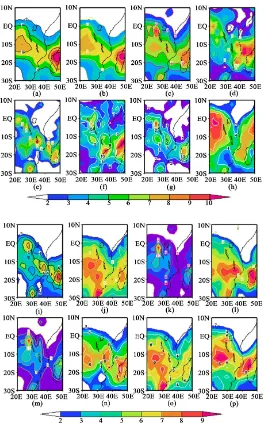
DOI: 10.4236/acs.2019.94038 616 Atmospheric and Climate Sciences Figure 9. The spatial distribution of precipitation anomalies in East Africa during the moderate flood event of September-November (SON) during 1994. (a) Observations, (b) S`SE, (c) EM, (d)-(p) Member models 1 to 13. (a) OBS_94; (b) SSE_94; (c) EM_94; (d) M01_94; (e) M02_94; (f) M03_94; (g) M04_94; (h) M05_94; (i) M06_94; (j) M07_94; (k) M08_94; (l) M09_94; (m) M10_94; (n) M11_94; (o) M12_94; (p) M13_94.
be defined as the average of the 1994 and 1997. The results are similar to those shown in Figure 9 and the SSE product emerges as a much forecast for the flood conditions in magnitudes and spatial distribution precipitations associated with warm ENSO events in Eastern Africa. From Figure 8, it is found that the 1996 drought that occurred during the SON season was predicted with good skill and it is useful to study the spatial distribution of the precipitation anomalies.
[image:17.595.243.509.64.492.2]DOI: 10.4236/acs.2019.94038 617 Atmospheric and Climate Sciences Figure 10. The spatial distribution of precipitation anomalies in East Africa during the drought event of September-November (SON) during 1996. (a) Observations, (b) SSE, (c) EM, (d)-(p) member models 1 to 13. (a) OBS_96; (b) SSE_96; (c) EM_96; (d) M01_96; (e) M02_96; (f) M03_96; (g) M04_96; (h) M05_96; (i) M06_96; (j) M07_96; (k) M08_96; (l) M09_96; (m) M10_96; (n) M11_96; (o) M12_96; (p) M13_96.
sector of East Africa. The superensemble forecast for the drought is shown in panel (b) and it captures the precipitation deficit well in magnitude and spatial coverage. The EM and member model forecasts are shown in panels (c) to (p) and it is found that none of these simulations compares with observations as fa-vorably as the SSE product.
DOI: 10.4236/acs.2019.94038 618 Atmospheric and Climate Sciences is characterized by droughts in Equatorial Eastern Africa and flooding in South-ern Africa. This regional scale climate feature can be recognized as a seesaw or dipole pattern. Additional discussions of the ENSO teleconnection with seasonal precipitation over the region may be found in [2] [32] [35] [36] among other studies and authors. It is useful to determine how well the superensemble pre-dicts this regional feature. In Eastern Africa, seasonal forecasts of climate are usually done SSTs and ENSO derived statistical relationships with precipitation. The statistical models cannot always give forecasts that are physically consistent with the large-scale mechanisms such as the atmospheric circulation characteris-tics and its modulation by regional and local scale processes. In this study, it is sufficient to focus on the skill of the SSE relative to the EM in forecasting this see-saw pattern in precipitation between Tropical East Africa and Southern Parts the larger Eastern Africa. By obtaining the average of the warm ENSO and cold ENSO events within the model data sets used in this study, Figure 11 summa-rizes the predictability of the regional precipitation gradient in which panels (a) and (d) show observations for the gradient pattern, panels (b) and (e) illustrate predictability by the SSE scheme and panels (c) and (f) show the performance of the EM. For the two scenarios, it is found that the multimodel superensemble simulates the “see-saw” in precipitation quite consistently with observations and outperforms the ensemble mean in getting accurately the magnitudes and spatial distribution of the season precipitation.
[image:19.595.243.503.434.655.2]Thus, the multimodel superensemble scheme can provide skill and robust re-sults that are spatially consistent over very large areas, such as seen in these
DOI: 10.4236/acs.2019.94038 619 Atmospheric and Climate Sciences results for the Eastern Africa ENSO precipitation dipole pattern. In global cli-mate models and also clicli-mate forecasts in many parts of Africa, SST anomaly patterns have been the most reliable long-range predictors. Accurate predictions of SST anomalies including ocean specific modes of variability, for example the Indian Ocean dipole mode [37] and ENSO SST anomalies in the equatorial Pa-cific are crucial for improvement of seasonal climate predictability, especially in Eastern Africa. The superesnsemble has been shown to provide accurate predic-tions of SST anomalies in all the tropical oceans [38]. Therefore, superensemble modeling can be used in prediction of all aspects of the climate system, with an accuracy that address the spatial and temporal evolution of the climate extremes better than anyone climate model. The prediction skill seen in the above results for dipole pattern of precipitation the larger Eastern Africa is a confirmation that this technique of climate modeling provides a robust means of predicting accu-rately regional scale climate extremes. Regional scale information of this nature and quality is a necessary input in the socio-economic planning and mobiliza-tion of resources for early warning, long-term advisories and policies acmobiliza-tions towards addressing of tribal/ethnic conflicts due to climatically driven resources in the Arid and Semi-Arid Lands (ASALs), for example fatal conflicts over grasslands and watering points between Semi-Nomadic communities living in Northern Kenya, Northeastern Uganda, and Southern Ethiopia during drought periods due to failure of seasonal rainfall. The construction of a multimodel su-perensemble forecasts can be the climate modeling solution to climate scientists working in Africa provided the worldwide centers with the facilities for conti-nuous improvements of specific climate models avail the real-time model data sets to scientists within Africa.
5. Conclusions
A comprehensive data from a suit of 13 global climate models has been used to construct superensemble climate forecasts in various regions of Africa. The mul-timodel superensemble technique that has been developed in Florida State Uni-versity is used. The approach removes the collective bias of the individual model forecasts by assigning weights to each of the member models based on their past performance and using those weights in a multiple linear regression to produce a consensus forecast for the variable of interest. In this study, the main objective is predictability of seasonal precipitation over various regions of Africa, and the potential improvements that can be achieved by using the superensemble rela-tive the skill attributes of the individual models and multimodel ensemble mean were the only forecast schemes available.
DOI: 10.4236/acs.2019.94038 620 Atmospheric and Climate Sciences the larger Eastern African and it has far reaching socio-economic implications on communities who are generally very poor and depend on rain-fed agriculture and agro-pastoral activities for food production. Improvements of prediction of seasonal climate anomalies that affect such huge areas is therefore a matter of priority in many parts of Africa.
The results have shown that even though the individual climate models and the ensemble mean simulate the basic annual and seasonal cycles of precipita-tion, the magnitudes and spatial distribution compare poorly with observations. In the simulation of the seasonal cycle of precipitation in the various regions of Africa, the superensemble product is found to be closest to the observed clima-tology, while the member models and ensemble mean simulations show big de-partures from observations. For the East Africa region, the superensemble may be said to provide an improvement of 18% above the multimodelensemble mean during the seasons March-May (MAM), June-August (JJA), September-November (SON), and December-February (DJF). During the DJF season, a regional scale north-south gradient of precipitation prevails between Tropical East Africa and South-eastern Africa. This regional scale climate pattern is a direct influence of the intertropical convergence zone (ITZC) across the African continent during this time of the year. The superensemble emerges as best among the member models and ensemble mean in the simulation of the north-south gradient of precipitation in the region.
When applied on a seasonal basis in various regions of Africa, the superen-semble gave precipitation forecasts that outperformed the member models and ensemble mean in skill scores. For example, in the July-September (JAS) preci-pitation in North Africa during 1989, the ensemble mean root mean square error (RMSE) was 1.5 mm/day, while the superensemble error was only 0.5 mm/day. In the region, the superensemble may be viewed as improving the performance of the ensemble mean by 67%. It is also found that in all the four regions of Africa, the RMSE of the superensemble product is lower, and different from the ensemble mean at more than 95% significance level. A lower RMSE indicates a superior performance.
re-DOI: 10.4236/acs.2019.94038 621 Atmospheric and Climate Sciences versed ENSO scenario, the superensemble forecasts stands with skill characteris-tics superior to those of the individual models and ensemble mean. The multi-model superensemble approach is therefore an innovative scheme for the pre-diction of regional scale climate extremes over the diverse regions of Africa.
When real time forecasts are made with several climate models, it is difficult to know in advance which among these models can be relied upon to give the most skilful climate forecast for the season and region of interest. It will help a lot if climatological hindcasts of global climate models are generated and arc-hived for longer periods. However, knowing that the superensemble has the highest skills always as illustrated in this study, it would be safer to rely on the superensemble in seasonal forecasts and for future projections of climate.
The multimodel superensemble should be useful for real time climate fore-casts over continental Africa and the surrounding ocean basins and future im-provements are certain from the advancement of physical climate modeling and more accurate observational analysis fields.
This approach and results herein imply that climate services centres world-wide and Africa in particular can make more objective use of model forecast da-ta sets, which is increasingly being freely availed by global producing centres (GPCs) for better quality and more objective regional climate services, especially over the sub-regions of Africa and even better processing of current climate change data sets being availed by projects like CMIP6 models.
Acknowledgements
Thanks to weather services and climate institutions round the world for making available various versions of their global model data sets in support of dynam-ical modeling and prediction research in Kenya and Africa in general. I am grateful to conducive scholarly environment provided by the University of Nai-robi-Kenya.
Conflicts of Interest
The author declares no conflicts of interest regarding the publication of this pa-per.
References
[1] Goddard, L. and Graham, E. (1999) The Importance of the Indian Ocean for Simu-lating Rainfall Anomalies over Eastern and Southern Africa. Journal of Geophysical Research: Atmospheres, 104, 19099-19116.https://doi.org/10.1029/1999JD900326 [2] Mutemi, J.N. (2003) Climate Anomalies over Eastern Africa Associated with
Vari-ous ENSO Evolution Phases. PhD Thesis, University of Nairobi, Nairobi.
[3] Karanja, F.K., Oludhe, C., Mutua, F.M. and Nyakwanda, W. (2000) Reducing the Impacts of Environmental Emergencies through Early Warning and Preparedness: The Case of El Niñ-Southern Oscillation (ENSO). Report of UNFIP/UNEP/NCAR/ WMO/DNDR/UNU.
DOI: 10.4236/acs.2019.94038 622 Atmospheric and Climate Sciences Rainfall and Their Prediction Potentials. International Journal of Climatology, 20, 19-46.
https://doi.org/10.1002/(SICI)1097-0088(200001)20:1<19::AID-JOC449>3.0.CO;2-0 [5] Ogallo, L.J. (1988) Relationship between Seasonal Rainfall in East Africa and the
Southern Oscillation. Journal of Climatology, 8, 31-43.
https://doi.org/10.1002/joc.3370080104
[6] Gates, W.L., Boyle, J.S., Covey, C., Dease, C.G., Doutriaux, C.M., Drach, R.S., Fi-orino, M., Gleckler, P.J., Hnilo, J.J., Marlais, S.M., Phillips, T.J., Potter, G.L., Santer, B.D., Sperber, K.R., Taylor, K.E. and Williams, D.N. (1999) An Overview of the Re-sults of the Atmospheric Model Intercomparison Project (AMIP I). Bulletin of the American Meteorological Society, 80, 29-55.
https://doi.org/10.1175/1520-0477(1999)080<0029:AOOTRO>2.0.CO;2
[7] Randall, D.A., Wood, R.A., Bony, S., Colman, R., Fichefet, T., Fyfe, J., Kattsov, V., Pitman, A., Shukla, J., Srinivasan, J., Stouffer, R.J., Sumi, A. and Taylor, K.E. (2007) Climate Models and Their Evaluation. In: Solomon, S., Qin, D., Manning, M., Chen, Z., Marquis, M., Averyt, K.B., Tignor, M. and Miller, H.L., Eds., Climate Change 2007: The Physical Science Basis. Contribution of Working Group I to the Fourth Assessment Report of the Intergovernmental Panel on Climate Change, Cambridge University Press, Cambridge, United Kingdom and New York.
[8] Krishnamurti, T.N., Kishtawal, C.M., LaRow, T.E., Bachiochi, D.R., Zhang, Z., Wil-liford, C.E., Gadgil, S. and Surendran, S. (1999) Improved Weather and Daily and Medium Range Climate Forecasts from Multi-Model Superensemble. Science, 285, 1548-1550.https://doi.org/10.1126/science.285.5433.1548
[9] Graham, R.J., Evans, A.D.L., Mylne, K.R., Harrison, M.S.J. and Robertson, K.B. (2000) An Assessment of Seasonal Predictability Using Atmospheric General Cir-culation Models. Quarterly Journal of the Royal Meteorological Society, 126, 2211- 2240.
[10] Palmer, T.N., Alessandri, A., Andersen, U., Cantelaube, P. and Davey, M. (2004) Development of a European Multi-Model Ensemble System for Seasonal to In-ter-Annual Prediction (DEMETER). Bulletin of the American Meteorological So-ciety, 85, 853-872. https://doi.org/10.1175/BAMS-85-6-853
[11] Doblas-Reyes, F.J., Hagedorn, R. and Palmer, T.N. (2005) The Rationale behind the Success of Multi-Model Ensembles in Seasonal Forecasting-II. Calibration and Combination. Tellus A, 57, 234-252.
https://doi.org/10.1111/j.1600-0870.2005.00104.x
[12] Krishnamurti, T.N., Kishtawal, C.M., Shin, D.W. and Williford, C.E. (2000) Multi-model Ensemble Forecasts for Weather and Seasonal Climate. Journal of Climate, 13, 4196-44216.
https://doi.org/10.1175/1520-0442(2000)013<4196:MEFFWA>2.0.CO;2
[13] Chaves, R.R., Ross, R.S. and Krishnamurti, T.N. (2005) Weather and Climate Pre-diction for South America Using a Multi-Model Superensemble. International Journal of Climatology, 25, 1881-1914.https://doi.org/10.1002/joc.1230
[14] Mutemi, J.N., Ogallo, L.A., Krishnamurti, T.N., Mishra, A.K. and Kumar, T.S.V.V. (2007) Multimodel Based Superensemble Forecasts for Short and Medium Range NWP over Various Regions of Africa. Meteorology and Atmospheric Physics, 95, 87-113. https://doi.org/10.1007/s00703-006-0187-6
[15] Yun, W.T., Stefanova, L., Mitra, A.K., Kumar, T.S.V.V., Dewar, W. and Krishna-murti, T.N. (2005) A Multi-Model Superensemble Algorithm for Seasonal Climate Prediction Using DEMETER Forecasts. TellusA, 57, 280-289.
DOI: 10.4236/acs.2019.94038 623 Atmospheric and Climate Sciences [16] Yun, W.T., Stefanova, L. and Krishnamurti, T.N. (2003) Improvement of the
Supe-rensemble Technique for Seasonal Forecasts. Journal of Climate, 16, 3834-3840. https://doi.org/10.1175/1520-0442(2003)016<3834:IOTMST>2.0.CO;2
[17] Lakeman, J.A. (1995) Climate Change 1995: The Science of Climate Change. Cam-bridge University Press, CamCam-bridge, 233-276.
[18] Krishnamurti, T.N., Bedi, H.S. and Hardiker, V.M. (1998) An Introduction to Global Spectral Modeling. Oxford University Press, New York, 253 p.
[19] Latif, M. (1987) Tropical Ocean Circulation Experiments. Journal of Physical Ocea-nography, 17, 246-263.
https://doi.org/10.1175/1520-0485(1987)017<0246:TOCE>2.0.CO;2
[20] Krishnamurti, T.N. and Bedi, H.S. (1983) Cumulus Parameterization and Rainfall Rates:Part III. Monthly Weather Review, 116, 583-599.
https://doi.org/10.1175/1520-0493(1988)116<0583:CPARRP>2.0.CO;2
[21] Grell, G.A. (1993) Prognostic Evaluation of Assumptions Used by Cumulus Para-meterizations. Monthly Weather Review, 121, 764-787.
https://doi.org/10.1175/1520-0493(1993)121<0764:PEOAUB>2.0.CO;2
[22] Chang, C.B. (1979) On the Influence of Solar Radiation and Diurnal Variation of Surface Temperatures on African Disturbances. Florida State University, Tallahas-see, FL.
[23] Lacis, A.A. and Hansen, J.E. (1974) A Parameterization for the Absorption of Solar Radiation in the Earth’s Atmosphere. Journal of the Atmospheric Sciences, 31, 118-133.https://doi.org/10.1175/1520-0469(1974)031<0118:APFTAO>2.0.CO;2 [24] Kiehl, J.T., Hack, J.J., Bonan, G.B., Boville, B.A., Williamson, D.L. and Rasch, P.J.
(1998) The National Center for Atmospheric Research Community Climate Model: CCM3.Journal of Climate, 11, 1131-1149.
https://doi.org/10.1175/1520-0442(1998)011<1131:TNCFAR>2.0.CO;2
[25] Kållberg, P., Berrisford, P., Hoskins, B., Simmons, A., Uppala, S., Lamy-Thépaut, S. and Hine, R. (2005) ERA-40 Project Report Series. ERA-40 Atlas. ECMWF ERA-40 Project Report Series. Shinfield Park, Reading, England.
[26] Hagedorn, R., Doblas-Reyes, F.J. and Palmer, T.N. (2005) The Rationale behind the Success of Multi-Model Ensembles in Seasonal Forecasting. Basic Concept. Tellus A, 57, 219-233.https://doi.org/10.1111/j.1600-0870.2005.00103.x
[27] Xie, P. and Arkin, P.A. (1997) Analysis of Global Monthly Precipitation Using Gauge Observations, Satellite Estimates, and Numerical Model Prediction. Journal of Climate,9, 840-858.
https://doi.org/10.1175/1520-0442(1996)009<0840:AOGMPU>2.0.CO;2
[28] Krishnamurti, T.N., Surendran, S., Shin, D.W., Correa-Torres, R.J., Kumar, T.S.V.V., Williford, E., Kummerow, C., Adler, R.F., Simpson, J., Kakar, R., Olson, W.S. and Turk, F.J. (2001) Real-Time Multianalysis-Multimodel Superensemble Forecasts of Precipitation Using TRMM and SSM/I Products. Monthly Weather Review, 129, 2861-2883.https://doi.org/10.1175/1520-0493(2001)129<2861:rtmmsf>2.0.co;2 [29] Dẻquẻ, M. (1997) Ensemble Size for Numerical Seasonal Forecasts. TellusA, 49,
74-86. https://doi.org/10.1034/j.1600-0870.1997.00005.x
[30] Wilks, D.S. (1995) Statistical Methods in the Atmospheric Sciences. Academic Press, New York, 467 p.
[31] Ross, R.S. and Krishnamurti, T.N. (2005) Reduction of Forecast Error for Global Numerical Weather Prediction by the Florida State University (FSU) Superensem-ble. Meteorology and Atmospheric Physics, 88, 215-235.
DOI: 10.4236/acs.2019.94038 624 Atmospheric and Climate Sciences [32] Ogallo, L.J. (1989) The Spatial and Temporal Patterns of the East African Seasonal Rainfall Derived from the Principal Component Analysis. International Journal of Climatology, 9, 145-167. https://doi.org/10.1002/joc.3370090204
[33] Krishnamurti, T.N. (1979) Tropical Meteorology. Compendium of Meteorology, Part 4, WMO Publication, Geneva, 428 p.
[34] Asnani, G.C. (1993) Tropical Meteorology. Sindh Colony, Aundh, Pune, India, 603 p. [35] Nicholson, S.E. (2017) Climate and Climatic Variability of Rainfall over Eastern
Africa. Reviews of Geophysics, 55, 590-635. https://doi.org/10.1002/2016RG000544 [36] Ropelewski, C.F. and Halpert, M.S. (1987) Global and Regional Scale Precipitation Patterns Associated with the El-Nino/Southern Oscillation. Monthly Weather Re-view 115, 1606-1626.
https://doi.org/10.1175/1520-0493(1987)115<1606:GARSPP>2.0.CO;2
[37] Saji, N.H., Goswami, B.N., Vinayachandran, P.N. and Yamagata, T. (1999) A Dipole Mode in the Tropical Indian Ocean. Nature, 401, 360-363.
https://doi.org/10.1038/43854
[38] Krishnamurti, T.N., Mitra, A.K., Kumar, T.S.V.V., Yun, W.T. and Dewar, W.K. (2006) Seasonal Climate Forecasts of the South Asian Monsoon Using Multiple Coupled Models. Tellus A, 58, 487-507.
DOI: 10.4236/acs.2019.94038 625 Atmospheric and Climate Sciences
Appendix
The root mean square error (RMSE) is given by:
(
)
2 1 21
1
RMSE N n n
n f o
N =
= −
∑
where:
N = number of grid points fn = forecast value at grid point n on =observed value at grind point n Student’s t-test
The significance level at which the RMSE of the superensemble is superior to that of the ensemble mean is expressed as a percentage and indicated at the top of each panel for each year of forecast in Figure 5 and Figure 6. The student’s t-test used is:
em sse
RMSE RMSE
s
d t
S − =
d d
S S
n
=
where Sd is the standard deviation of the RMSEs within an ensemble of n mem-bers.
1 2
, 1
s
t t −α n