Research on Rosenbrock Function Optimization Problem Based on Improved Differential Evolution Algorithm

(1)

https://www.scirp.org/journal/jcc ISSN Online: 2327-5227

ISSN Print: 2327-5219

DOI: 10.4236/jcc.2019.711008 Nov. 29, 2019 107 Journal of Computer and Communications

Research on Rosenbrock Function Optimization

Problem Based on Improved Differential

Evolution Algorithm

Jian Ma, Haiming Li

*

School of Computer Science and Technology, Shanghai University of Electric Power, Shanghai, China

Abstract

The Rosenbrock function optimization belongs to unconstrained optimiza-tion problems, and its global minimum value is located at the bottom of a smooth and narrow valley of the parabolic shape. It is very difficult to find the global minimum value of the function because of the little information pro-vided for the optimization algorithm. According to the characteristics of the Rosenbrock function, this paper specifically proposed an improved differen-tial evolution algorithm that adopts the self-adaptive scaling factor F and crossover rate CR with elimination mechanism, which can effectively avoid premature convergence of the algorithm and local optimum. This algorithm can also expand the search range at an early stage to find the global minimum of the Rosenbrock function. Many experimental results show that the algo-rithm has good performance of function optimization and provides a new idea for optimization problems similar to the Rosenbrock function for some problems of special fields.

Keywords

Differential Evolution, Rosenbrock Function, Self-Adaptive Mutation, Elimination Mechanism

1. Introduction

Differential evolution (DE) is a simple yet powerful search technique introduced by Storn and Price in 1995 [1]. It soon became a popular tool for solving global optimization problems because of several attractive features like having fewer control parameters, ease in programming, efficiency, etc. DE has a very special connection with artificial life, especially evolutionary algorithms. DE and

par-How to cite this paper: Ma, J. and Li, H.M. (2019) Research on Rosenbrock Function Optimization Problem Based on Improved Differential Evolution Algorithm. Journal of Computer and Communications, 7, 107-120. https://doi.org/10.4236/jcc.2019.711008

Received: September 20, 2019 Accepted: November 26, 2019 Published: November 29, 2019

http://creativecommons.org/licenses/by/4.0/

(2)

DOI: 10.4236/jcc.2019.711008 108 Journal of Computer and Communications

ticle swarm optimization (PSO) are optimization algorithms based on collective intelligence theory [2]. They all use collective intelligence to optimize the result of searching, which comes from individual cooperation and competition within the group. However, compared to the evolutionary algorithm, DE retains the global search strategy based on population and uses real number coding, diffe-rential-based simple mutation operation and one-to-one competitive survival strategy, which reduces the complexity of genetic operations. At the same time, DE has special memory ability to track current search status dynamically to ad-just the strategy of search. This capability indicates that the DE algorithm has strong global convergence ability and robustness without relying on the feature information of the problem, and the DE algorithm is suitable for solving opti-mization problems that cannot be solved by conventional mathematical pro-gramming methods in complex environments. Therefore, it is very academic and engineering value to conduct theoretical and applied research on DE [3], as an efficient parallel search algorithm.

In the minimization of the function, the phenomenon of “super valley” often occurs (at least in the local range) on the contour plane of the objective function. This shape is similar to the parabola with an upward opening. The global mini-mum value of the objective function is located at the bottom of the narrow val-ley. The optimization algorithm should have the ability to gradually approach the global minimum of the objective function along a narrow valley, and the Rosenbrock function of Rosenbrock, as a typical test function, was created for testing whether the optimization algorithm has this capability of searching the global minimum [4].

Many optimization algorithms now have a good optimization performance for most test functions, but much literature shows that many efficient algorithms and even many intelligent search algorithms are difficult to find global mini-mum values for the optimization of the Rosenbrock function, such as gradient descent, genetic algorithm (GA), particle swarm optimization (PSO) [5]. Specif-ically, for the gradient descent: when the objective function f(x) is minimized by the gradient descent, the gradient of the function is the vector in the direction of maximum local growth of f(x), and the opposite direction of the vector is the steepest downward direction. Because at point x, the negative gradient of f(x) points to the direction in which f(x) decreases the fastest for each component of

(3)

This paper proposes an improved differential evolution algorithm with self- adaptive mutation and control parameters to solve this kind of problem and op-timize the characteristic design of the Rosenbrock function. In this algorithm, the scaling factor F can be adaptively changed by the previous learning expe-rience, and the level of the crossover rate CR depends on the fitness value of the individual. Experiments show that the improved DE algorithm has better con-vergence speed and accuracy than other types of improved schemes.

2. Basic Differential Evolution Algorithm

Starting from a population of randomly initialized solutions, the DE algorithm employs simple mutation and crossover operators to generate new candidate solutions and utilizes a one-to-one competition scheme to deterministically de-cide whether the offspring will replace their parents in the next generation. The steps of the standard DE algorithm are as follows:

1) Population initialization

The matrix X defining N × D is used to store the data of the current popula-tion, where D is the dimension of the individual in the population, N is the size of the population. At first, it randomly generates N × D data obeying the uni-form distribution law and satisfying the specific constraint conditions. Put them into the matrix X to form the initial population

( )

0

{

1

( )

0 , 2

( )

0 , , N

( )

0

}

X = X X  X .

2) Variation operation

Let the population size be N, the current evolutionary individual is represented by X ti

( )

(i=1, 2,,N) and t is the current number of evolutions. Randomly

select three different individuals from the current evolutionary group and meet the conditions r r r1, ,2 3∈

{

1, 2,,N

}

. Individual Xr2

( )

t , Xr3

( )

t and difference

( )

2 3

r r

X t −X t are regarded as the disturbance factors of Xr1

( )

t . Add the

fac-tors and Xr1

( )

t to obtain the current mutant individual V ti

( )

, as shown in

Eq-uation (1):

( )

(

2

( )

3

( )

)

i ri r r

V t =X t +F X t −X t (1)

where F is the scaling factor that controls the disturbance factor. Individuals in a group are composed of D components, then variant individuals V ti

( )

also

com-posed of D components, so V ti

( )

=

(

vr1

( )

t ,vr2

( )

t ,,viD

( )

t

)

.

3) Crossover operation

Generate random integers r4∈

{

1, 2,,D

}

. The discrete variant individual

( )

i

V t crosses the current evolutionary individual X ti

( )

to obtain an intermediate

test individual U ti

( )

, which will compete with the X ti

( )

for the selection

op-eration and U ti

( )

consists of D component, U ti

( )

=

(

ui1

( )

t u, i2

( )

t ,,uiD

( )

t

)

.

The jth component (the chromosome in the individual) is as shown in Equation (2):

( )

4

0,1 or

ij ij

ij

v t randj CR j r

u t

v t randj CR j r

≤ =

 

> ≠

(4)

{

}

4 1, 2, ,

r ∈  D and randj

( )

0,1 represents a uniformly distributed random

number obeying (0,1), which can guarantee that the individual is mutated V ti

( )

at least one dimension component exists in the test individual U ti

( )

to ensure

the effectiveness of the mutation operation. CR∈

[ ]

0,1 is the probability of

crossover. The lower the probability of CR, the similarity of the intermediate test individual U ti

( )

for current evolutionary individual X ti

( )

is greater. This will

help ensure the diversity of the population and the global optimization of the algo-rithm.

4) Selection operation

In the case of seeking a minimum solution, the smaller the fitness value, the better. If the fitness value of U ti

( )

is less than the fitness value, the intermediate

individual U ti

( )

will replace the current individual X ti

( )

with the new

indi-vidual X ti

(

+1

)

. Otherwise, the current evolutionary individual X ti

( )

will

inhe-rit directly into the next generation. If the individual fitness value is f X t

(

i

( )

)

,

the selection operation can be expressed as follows (3):

(

)

( )

(

( )

)

(

( )

)

( )

(

( )

)

(

( )

)

if 1

if

i i i

i

i i i

U t f U t f X t

X t

X t f U t f X t

 ≤

 + = 

>

 (3)

5) Evaluation

In summary, the DE algorithm has the following advantages:

a) The algorithm is generic and does not depend on the problem information; b) The algorithm principle is simple and easy to implement;

c) Group search, with the ability to memorize the optimal solution of individ-uals;

d) Collaborative search, with the ability to further search using individual lo-cal information and group global information guidance algorithms;

e) It is easy to mix with other algorithms to construct an algorithm with better performance.

The search performance of the DE algorithm depends on the balance between the global exploration of the algorithm and the local development capability, which depends to a large extent on the selection of the control parameters of the algorithm, including population size, scaling factor and crossover probability. Compared with other evolutionary algorithms, the DE algorithm requires fewer parameters to adjust. It is necessary to select reasonable parameters for the guid-ance of selection.

3. The Analysis of the Rosenbrock Function

(5)

3.1. Definition of the Rosenbrock Function

The Rosenbrock function is defined as follows:

( ) (

)

2

(

₂

)

2

, 1 100

f x y = −x + y−x (4)

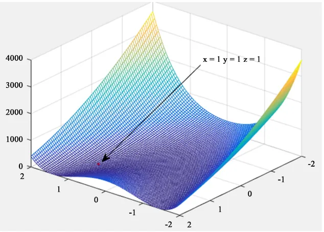
Each contour of the Rosenbrock function is roughly parabolic, whose global minimum is also in a parabolic valley (banana-type valley). It is easy to find this valley but quite difficult to find the minimum of the whole domain because the value in the valley does not change much.

The global minimum of the function is at (x, y) = (1, 1) and the value is f(x, y) = 0. Sometimes the coefficient of the second term (100 in the above formula) is different, but it does not affect the position of the global minimum. This paper mainly focuses on the Rosenbrock function in the two-dimensional case.

The three-dimensional map of the two variables of the Rosenbrock function is shown in Figure 1.

The more complex form of Rosenbrock function under multivariate [6] as fol-lows:

( )

1

(

)

2

(

2

)

2

1

1 1 100 ,

N N

i i i

i

f x =

∑

=− _ −x + x+ −x _ ∀ ∈x R (5)

It can be proved that when N = 3, this form of Rosenbrock function has only a minimum value, and the position is

(

1,1,1

)

, in 4≤N≤7, there are only two

minimum values. When all variables are 1, there is a global minimum

(

)

(

x x1, 2,,xN = −1,1,,1

)

. There is a local minimum nearby. This result is

[image:5.595.216.533.480.707.2]

ob-tained after the gradient of the function is zero. The Rosenbrock function is an unconstrained function optimization problem, which exhibits the characteristics of a multimodal function with a dimension greater than 3 and a unimodal indi-visible function with other dimensions.

(6)

3.2. The Analysis of the Rosenbrock Function

As you can see in Figure 1, the global minimum of the Rosenbrock function is at the bottom of a valley with a smooth and narrow parabola shape. It is difficult for general optimization algorithms to distinguish the search direction because of the less search information provided. It becomes difficult to find the global minimum value and easy to fall into a local optimum on one side of the valley. In the final search phase, these algorithms cannot jump out when the algorithm optimizes the Rosenbrock function.

This paper proposes a further improvement of the original differential evolu-tion algorithm, which combines the multi-strategy crossover operaevolu-tion and the self-adaptive dynamic adjustment algorithm parameters so that the algorithm takes into account both global search and local search. The new algorithm im-proves the convergence speed and accuracy of the optimization on the Rosen-brock function. The test results below verify the superiority of the algorithm.

4. Improved Differential Evolution Algorithm

4.1. Scaling Factor

F

By literature [7], it can be seen that when the scaling factor F is between [0.5, 1], the algorithm obtains better results. When F < 0.5or F > 1, the quality of the so-lution obtained by the algorithm is not high. And the literature shows that the average optimal value is ideal for almost all test functions at F = 0.5. Therefore, we take the benchmark value Fmin =0.5,Fmax =1 in the paper.

It can be known from Equation (1) that the value of F directly affects the con-vergence speed and concon-vergence of the algorithm: the scaling factor F controls the amplitude of the difference vector, and its value also affects the convergence and convergence speed. When F is small, the convergence speed is faster, but if it is too small, it tends to converge to the non-optimal solution; if F is large, it is conducive to convergence to the optimal solution, but the convergence speed is slower.

We need to maintain the diversity of the population in the initial stage of the search, and we should get as many individuals as possible globally optimal when doing a global search. We should also strengthen the ability of local search in the later stage of the search to improve the accuracy of the algorithm.

Therefore, we take such a measure for the value of F: The previous F takes a larger value to increase the mutation rate and ensure the ability of global search. And we reduce the F as the number of iterations increases, which can improve the ability of local search. We can propose an improved scheme of self-adaptive

F: By literature [8], a linearly decreasing

(

max min

)

max

t F F

F F

T −

= − ₍F_max and

min

F are the maximum and minimum values of F, t is the current number of

(7)

was proposed: max

(

max min

)

2

max g

F F F F

G

 

= − − _ _

  (g is the current number of

iterations, Gmax is the maximum number of iterations), the function of the

strategy is similar to a parabola with an opening down.

This paper uses an exponential declining strategy that is flatter and smoother than the first two.

1 1

e

0 2

T

T t

F F

₋   _{+ −}  

∗

= (6) In the above formula, F0 is equivalent to Fmin, t and T are the current

num-ber of iterations and the maximum numnum-ber of iterations, respectively. At the be-ginning of the algorithm, the self-adaptive mutation operator F is 2F0, which

means that the individual diversity can be maintained at the initial stage because of a large mutation rate; as the algorithm progresses, the mutation rate decreases gradually and will be close to F0 at the end of the algorithm, thus avoiding the

destruction of the optimal solution.

4.2. Crossover Rate

CR

The size of the crossover rate CR has a great influence on the convergence and convergence speed of the algorithm. It can be seen from Equation (2) that the larger the value of CR, the more Vi(t) contributes to Ui(t), which means that

there will be more variant individuals in the crossover operation. This trend is conducive to opening up new space and accelerating convergence.

However, the mutated individuals tend to be the same at a later stage (the self-adaptive values of the mutated individuals tend to be the same), which is not conducive to maintaining diversity, so it is easy to fall into the local optimal so-lution, and the stability of this kind of algorithm is poor; the smaller the value of

CR, the more Xi(t) contributes to Ui(t). In this way, the ability of the algorithm

to develop new space is weakened, and the convergence speed is relatively slow, but it is beneficial to maintain the diversity of the population (retaining the original individual characteristics), and thus the algorithm has a higher success rate. Therefore, we should choose to preserve the diversity of the population more stable in the early stage, and develop slowly, gradually increasing the CR to accelerate the accurate convergence in the later stage, and not easily fall into the local optimum.

By literature [10], four improvement strategies were proposed to improve the original fixed value CR. As a result, the optimization performance of the open-up parabola form is the best. The parameters are as follows:

(

max min

)

2 min

max g

CR CR CR CR

G

 

= − _ _ +

  (7)

max, min, , max

CR CR g G are the maximum and minimum values of CR, the

(8)

eva-DOI: 10.4236/jcc.2019.711008 114 Journal of Computer and Communications

luates the fitness of the function in the final selection. Is it possible to filter the mutated individuals in advance at the crossover operation, which provides more opportunities for excellent individuals to be selected at the crossover opera-tion; while disadvantaged individuals are given a lower probability and constantly being eliminated. Therefore, this paper proposes a kind of elimination mechan-ism based on the fitness of individuals (taking the minimum value as an exam-ple):

(

)

min max min

max

min

, if

, otherwise

i av

i av av

f f

CR CR CR f f

f f

CR

−

 ₊ ₋ _∗ _<

 ₋

=   

(8)

Set up a CR with maximum and minimum values called CRmax,CRmin. At the

same time, the average value of all fitness functions is calculated at each iteration

av

f and search for maximum fitness fmax. We use a mechanism for self-adaptive

CR regulation at the crossover operation:

Suppose we are looking for a global minimum. If the average value of the population fav is lower than the current fitness value of the individual fi, we

can treat this individual as a dominant individual. The crossover rate CR for the individual will increase with the degree of approximation to the maximum fit-ness. If the average value of the population fav is higher than the current

fit-ness value of the individual fi, we can treat this individual as an inferior

indi-vidual. The crossover rate CR for the individual will be set to the lowest CRmin.

Therefore, the dominant individual will be continued, and the inferior individu-al will graduindividu-ally decrease. The method individu-also follows the principle that the CR in-creases with the number of iterations.

As the algorithm reaches the end, the better fitness value of the function will be retained, the CR will be closer to the minimum value of the current iteration, which will help accelerate the convergence of the algorithm and improve the ac-curacy. The following Figure 2 shows the flow chart of the improved differential evolution algorithm.

We can call this strategy of simultaneously improved F-CR parameters as IEDE (Index-Elimination Differential Evolution Algorithm).

5. Experimental Results and Performance Analysis

5.1. Parameter Settings

In the experiment, we select the standard DE algorithm and the improved algo-rithm for performance test comparison. The parameters selected in the experi-ment are as follows: the population size is N = 5D - 10D and N = 50 in this pa-per. CR = 0.5, F0= 0.5, fmin = 0.5, fmax= 1, CRmin = 0.3, CRmax = 0.9 in the

(9)

[image:9.595.216.530.67.632.2]

DOI: 10.4236/jcc.2019.711008 115 Journal of Computer and Communications Figure 2. Flow chart for the improved DE algorithm.

5.2. Experimental Results and Performance Analysis

(10)

[image:10.595.239.508.70.288.2]

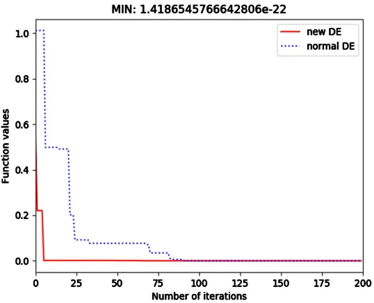
DOI: 10.4236/jcc.2019.711008 116 Journal of Computer and Communications Figure 3. Performance comparison of the two algorithms.

It can be seen from Figure 3 that the fitness of the newly improved differential evolution algorithm is closer to the optimal value (f = 0) than the standard diffe-rential evolution algorithm, and the best solution of this iteration in the figure is (x0, x1) = (0.9999999999935465, 0.9999999999860919), the final function value is

1.4186545766642806e − 22.

At the same time, we perform each algorithm of the other literature20 times and record the number of times it takes to reach the number of stable iterations to verify the superiority of the newly improved differential evolution algorithm. The results are shown in Table 1 and Table 2.

It can be seen from Table 2 that in the two improved schemes of the crossover rate CR, the CR-elimination mechanism is obviously superior to the CR para-bolic line, and it has achieved excellent results. It can be seen from the compari-son of the standard deviation that the standard deviation corresponding to the

CR-elimination mechanism is the smallest, indicating that the scheme has high repeatability.

Among three schemes of the scaling factor F, the effect of the F-parameter in the exponential form is better than that of the linear and parabolic methods (we adopt the control variable method: The CR is consistent with the parameters in the standard DE algorithm when we test F), but the iteration cost is more than the standard DE algorithm. This is because the self-adaptive characteristics of the F parameter are not reflected when the dimension is low, and the global op-timum can be easily found without changing the F.

(11)

[image:11.595.210.539.91.434.2]

DOI: 10.4236/jcc.2019.711008 117 Journal of Computer and Communications Table 1. The number of iterations required for each scheme to stabilize.

Experiment

number Normal DE F-linear [8] F-parabola [9] F-index CR-parabola [10] CR-elimination

1 88 103 126 101 146 34

2 94 166 143 132 150 30

3 89 98 193 119 132 44

4 81 142 161 115 135 26

5 87 140 160 132 93 43

6 88 72 141 110 113 28

7 125 109 144 111 112 27

8 68 123 172 127 131 38

9 86 112 131 120 135 26

10 95 115 157 129 118 20

11 93 105 145 133 117 46

12 86 129 150 118 145 50

13 113 127 133 106 146 50

14 96 162 132 109 152 50

15 77 132 129 117 139 33

16 75 149 152 85 139 38

17 89 133 98 144 166 49

18 101 158 157 155 166 49

19 97 139 134 113 151 42

20 90 140 160 136 173 35

Table 2. Experimental results under different improvement schemes.

Algorithm _{number of iterations}The maximum _{number of iterations}The average Minimum number _{of iterations} _deviationStandard

Normal DE 125 90.9 68 12.57357

F-linear [8] 166 127.7 72 23.60664

F-parabola [9] 193 145.9 98 19.94967

F-index 155 120.6 85 15.90895

CR-parabola [10] 173 137.95 93 20.19764

CR-elimination 50 31 20 9.62945

Normal DE refers to the standard DE algorithm without any changes; F-linear refers to changing F to

self-adaptive ( max min)

max

t F F

F F

T −

= − ; F-parabola refers to changing F to self-adaptive

( ) 2

max max min max

g

F F F F

G   = − −  

  ; F-index refers to changing F to self-adaptive

1 1 e 0 2 T T t F F −     _{+ −}   ∗

= ; CR-parabola

refers to changing CR to self-adaptive ( )

2

max min min

max

g

C C C CR

G R= R − R   +

  ; CR-elimination refers to

changing CR to self-adaptive min ( max min)

max min , if , otherwise i av i av av f f

C CR CR f f

f f

CR R CR

−

 ₊ ₋ _∗ _>

 ₋

=   

[image:11.595.209.538.466.591.2]

(12)

third round of testing is performed, taking D = 10, and the maximum number of iterations is 3000. We perform 20 times for each scheme and calculate the mean and standard deviation.

The experimental results are shown in Table 3, Table 4 below.

[image:12.595.234.511.238.456.2] [image:12.595.236.511.491.705.2]

It can be seen from the table that the standard DE algorithm cannot adapt to the computational difficulty brought by high-dimensional with the improvement of the dimension. At this time, the self-adaptive change advantage of F is re-flected. The original standard algorithm cannot meet the requirements of high- dimension, so we draw a graph comparison in these three schemes. As shown in

Figure 4 and Figure 5 below.

Figure 4. Changing curves of fitness value under three schemes (D = 5).

(13)

[image:13.595.210.541.89.187.2]

DOI: 10.4236/jcc.2019.711008 119 Journal of Computer and Communications Table 3. Experimental results at D = 5.

Algorithm Mean Standard deviation

Normal DE 852 60.25529

F-index 373 30.12806

F-parabola [9] 400 49.33322

F-linear [8] 470 49.09888

Table 4. Experimental results at D = 10.

Algorithm Mean Standard deviation

Normal DE 2456 195.3286

F-index 1239 181.0064

F-parabola [9] 1440 173.6327

F-linear [8] 1478 203.6981

We can see from Figure 4 and Figure 5 that in the three improved schemes, the improved DE algorithm in the F-index form proposed in this paper takes the least number of times to achieve stable iteration. When D = 5, the efficiency of the IEDE is increased by 128.4% compared with the standard DE algorithm, and the standard deviation is the lowest among the four schemes, which means that the scheme of the IEDE is the most efficient and stable, and the repeatability of the IEDE is higher than other schemes. It can be seen that the improved DE al-gorithm (IEDE) using the F-index-CR elimination mechanism can effectively improve the operation speed of the original algorithm.

6. Conclusion

[image:13.595.210.540.223.316.2]

(14)

Conflicts of Interest

The authors declare no conflicts of interest regarding the publication of this pa-per.

References

[1] Price, K. (1996) Differential Evolution: A Fast and Simple Numerical Optimizer.

Biennial Conference of the North American Fuzzy Information Processing Sociey, Berkeley, 19-22 June 1996, 524-527.

[2] Lu, X., Ke, T., Sendhoff, B. and Yao, X. (2014) A New Self-Adaptation Scheme for Differential Evolution. Neurocomputing, 146, 2-16.

https://doi.org/10.1016/j.neucom.2014.04.071

[3] Liu, B., Wang, L. and Jin, Y. (2007) Advances in Differential Evolution. Kongzhi yu Juece/Control and Decision, 22, 721-729.

[4] Rosenbrock, H.H. (1960) An Automatic Method for Finding the Greatest or Least Value of a Function. The Computer Journal, 3, 175-184.

https://doi.org/10.1093/comjnl/3.3.175

[5] Kennedy, J. and Eberhart, R. (1995) Particle Swarm Optimization. Proceedings of IEEE International Conference on Neural Networks, Perth, Australia, 27 Novem-ber-1 December 1995, 1942-1948.

[6] Yang, X.S. and Deb, S. (2010) Engineering Optimization by Cuckoo Search. Inter-national Journal of Mathematical Modelling and Numerical Optimisation, 1, 330-343.

https://doi.org/10.1504/IJMMNO.2010.035430

[7] Storn, R. (1996) On the Usage of Differential Evolution for Function Optimization.

Biennial Conference of the North American Fuzzy Information Processing Sociey, Berkeley, 19-22 June 1996, 519-523.

[8] Gao, Y.L. and Liu, J.F. (2008) Adaptive Differential Evolution Algorithm. Journal of Hebei University of Engineering, 8, 11-14.

[9] Xiao S.-J. and Zhu, X.-F. (2009) A Modified Fast and Highly Efficient Differential Evolution Algorithm. Journal of Hefei University of Technology (Natural Science), 32, 1700-1703.