Does turbulence determine the initial mass function?

Does turbulence determine the initial mass function?

David Liptai,

Daniel J. Price,

James Wurster

and Matthew R. Bate

1_{School of Physics and Astronomy, Monash University, Clayton, VIC 3800, Australia}

2_{School of Physics, University of Exeter, Stocker Road, Exeter EX4 4QL, UK}

Accepted 2016 October 25. Received 2016 October 24; in original form 2016 August 28

A B S T R A C T

We test the hypothesis that the initial mass function (IMF) is determined by the density probability distribution function (PDF) produced by supersonic turbulence. We compare 14 simulations of star cluster formation in 50 Mmolecular cloud cores where the initial turbu-lence contains either purely solenoidal or purely compressive modes, in each case resolving fragmentation to the opacity limit to determine the resultant IMF. We find statistically indis-tinguishable IMFs between the two sets of calculations, despite a factor of 2 difference in the star formation rate and in the standard deviation of log (ρ). This suggests that the density PDF, while determining the star formation rate, is not the primary driver of the IMF.

Key words: brown dwarfs – stars: formation – stars: low-mass – stars: luminosity function, mass function.

1 I N T R O D U C T I O N

Two decades of theoretical studies have established that a lognormal density probability distribution function (PDF) is the defining

char-acteristic of supersonic turbulence (e.g. Vazquez-Semadeni1994;

Nordlund & Padoan1999; Ostriker, Gammie & Stone1999; Klessen

2000; Kritsuk et al.2007; see review by Elmegreen & Scalo2004).

In particular, numerous studies (e.g. Padoan, Nordlund & Jones 1997a; Lemaster & Stone 2008; Price, Federrath & Brunt2011;

Molina et al.2012) have shown that the density variance is

propor-tional to the Mach number, giving

σ2 lnρ =ln

1+b2_M2_{, (1)}

whereσlnρis the standard deviation in the logarithm of the density

(i.e. the ‘width’ of the PDF),Mis the root-mean-square (RMS)

Mach number andb is a constant of order unity related to the

mixture of solenoidal and compressive modes in the velocity field

(e.g. Federrath, Klessen & Schmidt2008; Federrath et al.2010).

Padoan & Nordlund (2002) proposed that the PDF determines the

IMF for low-mass stars (M<1 M), based on the observation that

the IMF is also lognormal at the low-mass end (e.g. Chabrier2003,

2005). Relating the PDF to the IMF is powerful because it enables

analytic theories of star formation (e.g. Krumholz & McKee2005;

Hennebelle & Chabrier2008,2009; Hopkins2012; Guszejnov &

Hopkins2015) which predict the IMF from the few parameters in

equation (1). Relating the initial mass function (IMF) to the statistics of turbulence explains the universal nature of the IMF in the Milky

Way (e.g. Bastian, Covey & Meyer2010), since nearby molecular

clouds show supersonic motions with seemingly universal scaling

_{E-mail:[email protected]}

relations (Zuckerman & Evans1974; Larson1981; Heyer & Brunt

2004).

Measurements of lognormal column density PDFs from

extinc-tion mapping (Lombardi, Alves & Lada2006; Lombardi, Lada &

Alves2008,2010) lend support to a direct relationship between the

PDF and the IMF. In particular, Kainulainen et al. (2009) showed

that star-forming clouds differ from non-star-forming clouds by the presence of a power-law tail in the column density PDF at high den-sities, suggesting that self-gravity merely converts the high-density end of the PDF into stars. The measured mass function of ‘cores’ also seems to mimic the stellar IMF, but shifted to higher masses, implying a one-to-one relationship between ‘cores’ and ‘stars’ with

an efficiency factor of∼0.3 (e.g. Motte, Andre & Neri1998; Testi &

Sargent1998; Luhman & Rieke1999; Johnstone et al.2000; Alves,

Lombardi & Lada2007; Nutter & Ward-Thompson2007; Enoch

et al.2008; Rathborne et al.2009; Chabrier & Hennebelle2010).

However, numerous studies have also cautioned or argued against a direct core mass function and IMF relationship (e.g.

Ballesteros-Paredes et al.2006; Goodwin et al.2008; Smith, Clark & Bonnell

2008,2009).

Alternatively, Bonnell et al. (1997) and Bate & Bonnell (2005)

proposed that the IMF is determined by ‘competitive accretion’ between low-mass fragments for a limited gas supply, with accretion truncated by the preferential ejection of low-mass stars and brown dwarfs from unstable multiple systems. This was demonstrated in the star cluster formation calculations of Bate, Bonnell & Bromm

(2003; hereafterBBB03). These were the first attempts to simulate

the IMF ‘directly’ by resolving the gravitational collapse to the opacity limit for fragmentation (the density at which radiation is

trapped by dust,ρ≈10−13_{g cm}−3_{, implying an increase rather than}

decrease in the Jeans mass with density, and hence the formation of

a single hydrostatic object; Low & Lynden-Bell1976; Rees1976).

2016 The Authors

via a lognormal distribution of mass accretion rates. Nevertheless, a connection may still exist.

Here, we investigate the PDF–IMF connection by simulating star formation in two initially identical sets of model clouds, set up with either purely solenoidal or purely compressive initial velocity fields. If the PDF determines the IMF, then we expect the IMFs to differ, since the PDFs should be very different. If the IMF is more due to

nurturethannature, the effect may be more minor. The main caveat to our study is that we assume impulsive rather than continuous turbulent driving.

Girichidis et al. (2011) performed a related study, along with other

variations in the initial conditions, and found that the shape of the IMF was unaffected by the type of turbulent driving. However, they

simulated more massive and denser clouds (M=100 MandR=

0.1 pc) and did not resolve to the opacity limit (sinks were inserted

at a scale of 40 au, compared to 5 au employed here and inBBB03).

We also perform a statistical study with multiple realizations of the initial velocity field in each case, compared to their single

realiza-tion. Lomax, Whitworth & Hubber (2015) recently compared the

effect of solenoidal versus compressive forcing in star formation

cal-culations, but focused on smaller cores (M=3 M;R=3000 au),

examining the effect on disc and binary fractions rather than the IMF.

While this paper was under review, an important and

comple-mentary study to ours was published by Bertelli Motta et al. (2016),

examining the correlation between the IMF and the statistics of turbulence using two sets of simulations where the turbulence was first driven to a steady state in a periodic box before ‘switching on’ gravity. These authors varied the Mach number as well as the

den-sity of the cloud, using a total mass of either 5750 Mor 516 M

in a 10 pc3_{or 3 pc}3_{domain, respectively. Their ‘high density’}

sim-ulations were resolved only to a density of 1.6×10−14_{g cm}−3_{, one}

order of magnitude less than the opacity limit, with sink particle radii of 100 au. They found no correlation between the Mach num-ber and the characteristic mass of the resulting IMF, concluding that the IMF is mainly determined by small-scale processes such as disc formation and fragmentation and not by turbulence driven at the scale of the cloud. However, studying the role of initial conditions in a clump with decaying turbulence remains important since this may be closer to the situation in dense cores prior to the onset of stellar feedback.

2 N U M E R I C A L M E T H O D

We use thePHANTOMsmoothed particle hydrodynamics (SPH) code

(Lodato & Price2010; Price & Federrath2010; Price2012). This

is the first application ofPHANTOMto star cluster formation.

2.2 Equation of state

We adopt a barotropic equation of stateP=Kργ. FollowingBBB03,

we prescribeγ =1 (i.e. isothermal) for densities lower than the

opacity limit for fragmentation (ρ =10−13 _gcm−3_{),γ = 7/5 for}

10−13_gcm−3_{< ρ <10}−10_gcm−3_{andγ=1.1 forρ >10}−10_gcm−3_.

We define the constantKto be such that the sound speed iscs=

1.84×104_{cm s}−1_{during the isothermal phase (i.e. 10 K assuming}

a mean molecular weightμ=2.46) and in theγ = 7/5 regime

such that the pressure remains continuous when γ changes. As

discussed by Bate (2009a), using a barotropic equation of state

overproduces low-mass stars and brown dwarfs compared to ob-servations, since the cold gas surrounding the protostars fragments

too readily (cf. Fig.6). Several groups (Bate2009b,2012; Offner

et al.2009; Commerc¸on et al.2010; Krumholz et al.2010) showed

that this can be solved by modelling radiation in the flux-limited diffusion approximation. However, simulations with radiation are expensive, precluding the kind of statistical study we perform here,

the radiation algorithm is not yet implemented in PHANTOM, and

a barotropic equation of state is sufficient to answer the question of whether the PDF influences the IMF. We also ignore magnetic fields which change the star formation rate and perhaps also the IMF

(Ostriker et al.1999; Heitsch, Mac Low & Klessen2001;

V´azquez-Semadeni, Kim & Ballesteros-Paredes2005; Tilley & Pudritz2007;

Price & Bate2008,2009; Myers et al.2014).

2.3 Velocity fields: solenoidal versus compressive driving

We impulsively drive turbulence in each cloud, as inBBB03, by

im-posing an initial supersonic turbulent velocity field. The amplitude

of the velocity fluctuations follow a power spectrumP(k)∝k−4_,

wherekis the wavenumber, in order to be consistent with Larson’s

scaling relation. We generate each field via a Fourier transform on

a 643_{grid, which is then interpolated on to the SPH particles. The}

coefficient of each Fourier mode is drawn from a Rayleigh distri-bution with each mode also given a uniform random phase between

[−π,π]. This is equivalent to sampling from a cylindrical bivariate

Gaussian (Dubinski, Narayan & Phillips1995).

To obtain a purely solenoidal velocity field, we take the curl of a vector field to produce a divergence-free velocity field. Similarly for a purely compressive velocity field, we take the gradient of a scalar field to produce a curl-free field. We compute the gradients in Fourier space. Velocities are normalized so that the initial kinetic energy is equal to the gravitational potential energy, giving an

ini-tial RMS Mach number ofM=6.4. We performed simulations

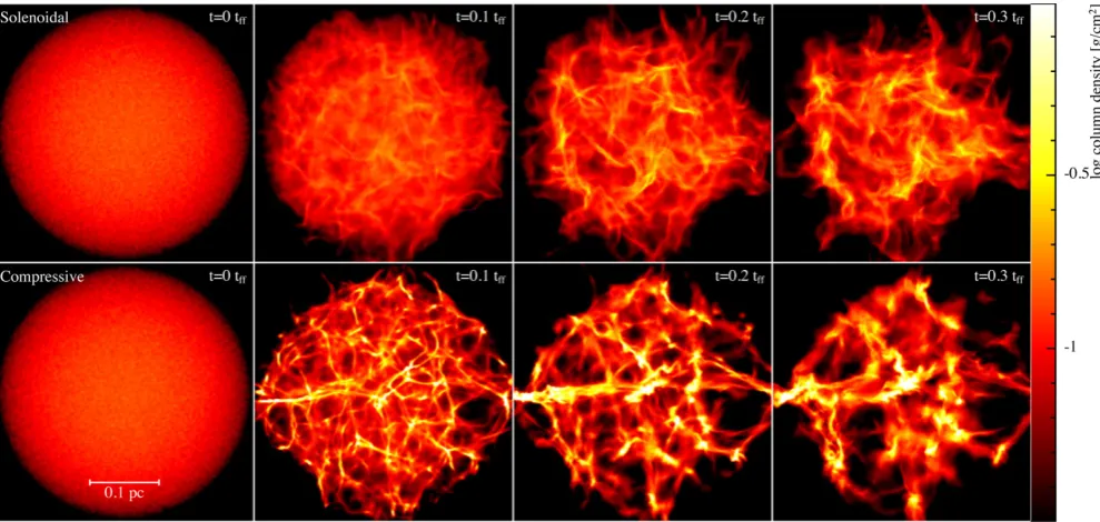
Figure 1. Evolution of column density during the gravitational collapse of two example 50 Mmolecular cloud cores with purely solenoidal (top) and purely compressive (bottom) initial turbulent velocity fields. The large-scale structure of the clouds is very different, with the compressive case showing a factor of 2 increase in the standard deviation of log (ρ) compared to the solenoidal case as well as stronger shocks and a faster onset to star formation. To obtain enough statistics to determine the IMF, we perform simulations using seven realizations of each type of driving, giving 14 simulations in total.

2.4 Sink particles

FollowingBBB03, we introduce sink particles (Bate, Bonnell &

Price1995) when the central density of pressure-supported

frag-ments reachesρs=10−11_{g cm}−3_{, two orders of magnitude higher}

than the opacity limit. Onceρs is exceeded and sink formation

conditions are satisfied, we replace gas particles within 5 au with a sink particle. Gas particles within 5 au are accreted if they pass checks for angular momentum and boundness, with their mass and momentum added to the sink. Gravity between sinks is softened within 4 au; gas particles are accreted without checks within this radius.

3 R E S U LT S

3.1 Column density evolution

Fig.1shows the evolution of column density fromt=0 tot=0.3tff

(left to right) in two representative calculations, using solenoidal

driving (top, as in BBB03) and compressive driving (bottom).

Shocks form quickly in both cases, due to the impulsive super-sonic velocity field, but are stronger in the compressive case,

driv-ing the formation of large-scale filaments after only 0.3tff. For the

solenoidal case,∇ ·v=0 initially by definition, so there are no

regions which initially promote collapse.

Fig. 2shows the subsequent small-scale fragmentation in the

compressive cloud, with the first protostar formed after just 0.2tff.

The process in all other clouds appears visually very similar. Gas flows into dense cores along filaments (e.g. G´omez &

V´azquez-Semadeni2014; Federrath2016; Klassen, Pudritz & Kirk2016;

Smith et al.2016), feeding young protostars via accretion discs. The

process is chaotic and dynamical, with close encounters between stars resulting in the destruction of accretion discs, and the ejection of smaller mass objects. Bound systems form and get destroyed by interactions on a very short time-scale. The stars live in a competitive

Figure 2. Snapshots of the evolution after the onset of star formation, show-ing column density in a 0.03 pc×0.03 pc inset for one of our compressively driven clouds. The star formation process is similar in solenoidal clouds, but occurs later and at a slower rate.

environment, where those which grow in mass quickly stay in the dense regions and accrete further material, whilst ejecting lower mass objects.

3.2 Comparison of PDFs

We computed the density PDFs by binning the particles into 2000

bins equally spaced between−10<log10(ρ)<10 in code units. We

then computed the standard deviation,σlnρ by fitting a lognormal

distribution to the PDF (usingscipy.optimize.curve_fit

in PYTHON). Note that the PDF computed in this way is weighted, rather than volume-weighted. Both volume- and mass-weighted PDFs are expected to be lognormal when the equation of state is approximately isothermal (Padoan, Jones & Nordlund 1997b; Passot & V´azquez-Semadeni 1998; Scalo et al. 1998;

Nordlund & Padoan1999; Ostriker, Stone & Gammie2001).

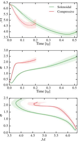
Figure 3. The time evolution of the RMS Mach numberM(top) and the mass-weighted standard deviation of the logarithm of densityσlnρ(middle). The lower panel shows the evolution in theσ–Mplane. Solid lines show the mean over all seven simulations of each type while the shaded error bars indicate the standard deviation between simulations.

Fig.3shows the time evolution of the (mass-weighted) RMS

Mach number,M(top panel) and standard deviation,σlnρ(centre

panel) for our entire set of calculations, with the solid lines showing the mean from the seven different simulations for each type of

velocity field and the shaded region shows the 1σstandard deviation.

The bottom panel shows the evolution in theM–σlnρplane. In both

the solenoidal and compressive clouds,Mdecays with time due

to the dissipation of energy by shocks, reaching a minimum before rising again once bound structures have formed.

Comparison of PDFs in decaying turbulence simulations is com-plicated by the time evolution of the velocity field. In our calcula-tions, the initial density field is uniform and the PDF thus develops in response to the initial turbulent velocity field. Since the clouds evolve on different time-scales, it is not particularly meaningful to compare their PDFs at the same time. Rather – for the purposes of our study – equation (1) suggests that they should be compared at

the same RMS Mach numberMso that the only difference is from

the different mixing parametersb.

The lower panel of Fig.3shows that the initial collapse of the

cloud roughly corresponds toσlnρ 2. Onceσlnρ reaches this

value,Mrises again once fragmentation begins. Also, the PDF is

no longer lognormal. We thus use the time interval whereσlnρ <

2 to compare the density PDFs prior to the onset of star formation. The standard deviation of the PDFs is different not only at the same time early in the evolution of the cloud, but also at the same RMS Mach number.

Fig.4shows the resultant PDFs computed at the time when all

calculations have the same RMS Mach number ofM=5.5, which

is whenσ differs most between the simulations. The difference

in the PDF produced by compressive versus solenoidal driving is

Figure 4. Comparison of the mass-weighted density PDFs for the two types of turbulent driving, compared at the same RMS Mach number of

M=5.5. Solid lines show the mean over all seven simulations of each type while shaded regions represent the 1σ deviations between different realizations.

Figure 5. Total mass in sink particles as a function of time for the two types of driving. The star formation rate is higher by a factor of 2 in the calculations employing compressive driving. The onset of star formation also occurs≈0.9 free-fall times earlier.

similar to that shown by e.g. Federrath et al. (2008,2010), except

that we show the mass-weighted version. Compressive driving pro-duces a broadening of the PDF caused by the collision of stronger shocks which in turn create larger variations in the density field. This demonstrates that our different choices of impulsive driving indeed drive significant differences in the density PDF prior to star formation.

3.3 Star formation rate

Fig.5shows the total stellar mass as a function of time, measured

by the mass in sink particles. The onset of star formation occurs

att≈0.2tffin the compressive case, compared tot≈1.1tffin the

solenoidal case. Once star formation starts in each calculation, the rate at which material is converted to stars is higher by a factor of

∼2 in the compressive clouds compared to the solenoidal cloud.

The overall efficiency of star formation is similar in both types of calculation over the time we have continued the simulations,

with≈15 per cent of the gas mass converted to stars. However,

the efficiency is higher on an absolute scale since this occurs over a shorter time-scale in the compressive case. Also, the end of the simulations does not mark the end of the star formation process since the mass in stars continues to increase.

3.4 Comparison of IMFs

Fig.6shows the IMFs from our simulations, combining all seven

realizations with solenoidal (left) and compressive driving (right),

Figure 6. Combined IMFs (blue and red histograms) from the seven solenoidal (left) and seven compressive (right) simulations. Solid/dashed lines show the empirically derived IMFs of Kroupa (2001) and Chabrier (2005) for comparison. While our simulations overproduce low-mass objects, consistent with Bate (2009a), the IMFs with either solenoidal or compressive driving are statistically indistinguishable, suggesting no direct link between the PDF (Fig.4) and the IMF.

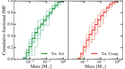
Figure 7. Cumulative IMFs, comparing solenoidal (left) to compressive (right). Thick bold lines show the mean of all realizations while the thinner lines show the results from individual calculations.

which have finished accreting (235 of 388 and 298 of 533 sinks for solenoidal and compressive, respectively) are shown in red, while the IMF of all stars is shown in blue. The lowest mass possible in

our calculations is≈0.005 Mfrom the opacity limit for

fragmen-tation, which sets the low-mass cutoff. The IMFs appear similar

to those shown inBBB03but with better statistics because of our

multiple realizations. Our IMFs are also similar to those found by

Bate (2009a) from one calculation of a 500 Mcloud. In particular,

we observe the statistically significant excess in low-mass stars and

brown dwarfs compared to the Kroupa (2001) and Chabrier (2005)

IMFs (dashed and solid lines, respectively) which occurs when a

barotropic equation of state is employed (e.g. Bate2009a,b).

There is no obvious difference between the IMFs produced by the different types of driving. Statistics confirm this – a Kolmogorov–

Smirnov test gives ap-value of 0.71 between the two distributions

when considering all sink particles, and ap-value of 0.98 when

considering only sinks which have finished accreting. This means that we cannot reject the hypothesis that the samples come from the same underlying distribution. Thus, while the type of driving changes the density PDF, the resultant IMFs are indistinguishable.

4 D I S C U S S I O N A N D C O N C L U S I O N S

We presented the results of 14 numerical simulations of the

gravita-tional collapse of 50 Mmolecular clouds, each impulsively driven

with a different random solenoidal or compressive velocity field to test the effect of the initial turbulence on the IMF. We resolved frag-mentation to the opacity limit, at which point sink particles were

inserted. By allowing the sink particles to accrete and grow in mass, we directly measured the masses of the resultant cluster of stars.

We found that while the initial turbulent velocity fields yielded different density PDFs during the initial collapse phase (before star formation begins), they had no significant effect on the IMF.

How-ever, the star formation rate was≈2 times greater in the

compres-sively driven clouds, with the onset of star formation occurring 0.9 free-fall times earlier. Our findings are consistent with Girichidis

et al. (2011), who found that their IMFs unchanged by the ratio

of solenoidal and compressive modes in the initial turbulence, and

with Bate (2009c) who found that using a different initial kinetic

power spectrum did not significantly alter the resulting IMF. The main caveat to our study is that we assumed impulsive turbu-lent driving, which does not produce a statistical steady state. Thus, it may be argued that the turbulent support present in the collapsing cores has already decayed by the time star formation occurs. Also, our density PDFs evolve in time and do not maintain the empir-ical relation between the variance, Mach number and the ratio of

solenoidal and compressive modes (equation 1; see Fig.3).

How-ever, the decaying regime is important as it may better represent

dense cores prior to star formation (e.g. Lada et al.2008) and thus

driving of the velocity field by outflows and radiative feedback. The best answer to the above caveat is provided in the

com-plementary study by Bertelli Motta et al. (2016). Although these

authors did not resolve the IMF to the opacity limit, they used clouds driven to a statistical steady state inside a periodic box, be-fore ‘switching on’ gravity to collapse the cloud. Importantly, the turbulence in their experiments was continually driven throughout the calculations, producing PDFs which match equation (1). De-spite this, in their ‘high density’ simulations which are most similar

to ours, Bertelli Motta et al. (2016) found no correlation between

the properties of the turbulence and the resulting shape of the IMF, which is consistent with our findings. Furthermore, the trends found in their ‘low density’ simulations, though of too low resolution to probe the IMF directly, were also not consistent with the predictions of existing analytic theories. The authors attribute the null result in their ‘high density’ simulations to the IMF being determined mainly by dynamical evolution of the fragments under the influence of self-gravity, which is also the case in our study. Thus, whether or not turbulence is driven or decaying, it would appear to have little or no influence on the IMF.

Truly realistic simulations require an understanding of the phys-ical source of turbulent driving in the interstellar medium. Our sim-ulations also did not include radiative transfer or magnetic fields,

Project DP130102078 and Future Fellowship FT130100034. We usedSPLASH(Price2007).

R E F E R E N C E S

Alves J., Lombardi M., Lada C. J., 2007, A&A, 462, L17

Ballesteros-Paredes J., Gazol A., Kim J., Klessen R. S., Jappsen A.-K., Tejero E., 2006, ApJ, 637, 384

Bastian N., Covey K. R., Meyer M. R., 2010, ARA&A, 48, 339 Bate M. R., 2009a, MNRAS, 392, 590

Bate M. R., 2009b, MNRAS, 392, 1363 Bate M. R., 2009c, MNRAS, 397, 232 Bate M. R., 2012, MNRAS, 419, 3115

Bate M. R., Bonnell I. A., 2005, MNRAS, 356, 1201 Bate M. R., Burkert A., 1997, MNRAS, 288, 1060

Bate M. R., Bonnell I. A., Price N. M., 1995, MNRAS, 277, 362

Bate M. R., Bonnell I. A., Bromm V., 2003, MNRAS, 339, 577 (BBB03) Bertelli Motta C., Clark P. C., Glover S. C. O., Klessen R. S., Pasquali A.,

2016, MNRAS, 462, 4171

Bonnell I. A., Bate M. R., Clarke C. J., Pringle J. E., 1997, MNRAS, 285, 201

Chabrier G., 2003, PASP, 115, 763

Chabrier G., 2005, Astrophys. Space Sci. Libr., 327, 41 Chabrier G., Hennebelle P., 2010, ApJ, 725, L79

Commerc¸on B., Hennebelle P., Audit E., Chabrier G., Teyssier R., 2010, A&A, 510, L3

Dubinski J., Narayan R., Phillips T. G., 1995, ApJ, 448, 226 Elmegreen B. G., Scalo J., 2004, ARA&A, 42, 211

Enoch M. L., Evans N. J., II, Sargent A. I., Glenn J., Rosolowsky E., Myers P., 2008, ApJ, 684, 1240

Federrath C., 2016, MNRAS, 457, 375

Federrath C., Klessen R. S., Schmidt W., 2008, ApJ, 688, L79

Federrath C., Roman-Duval J., Klessen R. S., Schmidt W., Mac Low M.-M., 2010, A&A, 512, A81

Girichidis P., Federrath C., Banerjee R., Klessen R. S., 2011, MNRAS, 413, 2741

G´omez G. C., V´azquez-Semadeni E., 2014, ApJ, 791, 124

Goodwin S. P., Nutter D., Kroupa P., Ward-Thompson D., Whitworth A. P., 2008, A&A, 477, 823

Guszejnov D., Hopkins P. F., 2015, MNRAS, 450, 4137 Heitsch F., Mac Low M.-M., Klessen R. S., 2001, ApJ, 547, 280 Hennebelle P., Chabrier G., 2008, ApJ, 684, 395

Hennebelle P., Chabrier G., 2009, ApJ, 702, 1428 Heyer M. H., Brunt C. M., 2004, ApJ, 615, L45 Hopkins P. F., 2012, MNRAS, 423, 2037

Larson R. B., 1981, MNRAS, 194, 809

Lemaster M. N., Stone J. M., 2008, ApJ, 682, L97 Lodato G., Price D. J., 2010, MNRAS, 405, 1212

Lomax O., Whitworth A. P., Hubber D. A., 2015, MNRAS, 449, 662 Lombardi M., Alves J., Lada C. J., 2006, A&A, 454, 781

Lombardi M., Lada C. J., Alves J., 2008, A&A, 489, 143 Lombardi M., Lada C. J., Alves J., 2010, A&A, 512, A67 Low C., Lynden-Bell D., 1976, MNRAS, 176, 367 Luhman K. L., Rieke G. H., 1999, ApJ, 525, 440

Molina F. Z., Glover S. C. O., Federrath C., Klessen R. S., 2012, MNRAS, 423, 2680

Motte F., Andre P., Neri R., 1998, A&A, 336, 150

Myers A. T., Klein R. I., Krumholz M. R., McKee C. F., 2014, MNRAS, 439, 3420

Nordlund Å. K., Padoan P., 1999, in Franco J., Carraminana A., eds, Inter-stellar Turbulence. Cambridge Univ. Press, Cambridge, p. 218 Nutter D., Ward-Thompson D., 2007, MNRAS, 374, 1413

Offner S. S. R., Klein R. I., McKee C. F., Krumholz M. R., 2009, ApJ, 703, 131

Ostriker E. C., Gammie C. F., Stone J. M., 1999, ApJ, 513, 259 Ostriker E. C., Stone J. M., Gammie C. F., 2001, ApJ, 546, 980 Padoan P., Nordlund Å., 2002, ApJ, 576, 870

Padoan P., Nordlund A., Jones B. J. T., 1997a, MNRAS, 288, 145 Padoan P., Jones B. J. T., Nordlund A. P., 1997b, ApJ, 474, 730 Passot T., V´azquez-Semadeni E., 1998, Phys. Rev. E, 58, 4501 Price D. J., 2007, PASA, 24, 159

Price D. J., 2012, J. Comput. Phys., 231, 759 Price D. J., Bate M. R., 2008, MNRAS, 385, 1820 Price D. J., Bate M. R., 2009, MNRAS, 398, 33 Price D. J., Federrath C., 2010, MNRAS, 406, 1659 Price D. J., Federrath C., Brunt C. M., 2011, ApJ, 727, L21

Rathborne J. M., Lada C. J., Muench A. A., Alves J. F., Kainulainen J., Lombardi M., 2009, ApJ, 699, 742

Rees M. J., 1976, MNRAS, 176, 483

Scalo J., Vazquez-Semadeni E., Chappell D., Passot T., 1998, ApJ, 504, 835 Smith R. J., Clark P. C., Bonnell I. A., 2008, MNRAS, 391, 1091 Smith R. J., Clark P. C., Bonnell I. A., 2009, MNRAS, 396, 830

Smith R. J., Glover S. C. O., Klessen R. S., Fuller G. A., 2016, MNRAS, 455, 3640

Testi L., Sargent A. I., 1998, ApJ, 508, L91 Tilley D. A., Pudritz R. E., 2007, MNRAS, 382, 73 Vazquez-Semadeni E., 1994, ApJ, 423, 681

V´azquez-Semadeni E., Kim J., Ballesteros-Paredes J., 2005, ApJ, 630, L49 Zuckerman B., Evans N. J., II1974, ApJ, 192, L149