Interface Dynamics in Planar Neural Field Models
S Coombes
∗1, H Schmidt
1, I Bojak
21School of Mathematical Sciences, University of Nottingham, Nottingham, NG7 2RD, UK. 2School of Psychology (CN-CR), University of Birmingham, Edgbaston, Birmingham B15 2TT, UK.
Email: S Coombes∗ stephen.coombes@nottingham.ac.uk; H Schmidt pmxhs@exmail.nottingham.ac.uk; I Bojak -i.bojak@bham.ac.uk;
∗Corresponding author
Abstract
Neural field models describe the coarse-grained activity of populations of interacting neurons. Because of the
laminar structure of real cortical tissue they are often studied in two spatial dimensions, where they are well
known to generate rich patterns of spatiotemporal activity. Such patterns have been interpreted in a variety of
contexts ranging from the understanding of visual hallucinations to the generation of electroencephalographic
signals. Typical patterns include localized solutions in the form of traveling spots, as well as intricate
labyrinthine structures. These patterns are naturally defined by the interface between low and high states of
neural activity. Here we derive the equations of motion for such interfaces and show, for a Heaviside firing rate,
that the normal velocity of an interface is given in terms of a non-local Biot-Savart type interaction over the
boundaries of the high activity regions. This exact, but dimensionally reduced, system of equations is solved
numerically and shown to be in excellent agreement with the full nonlinear integral equation defining the neural
field. We develop a linear stability analysis for the interface dynamics that allows us to understand the
mechanisms of pattern formation that arise from instabilities of spots, rings, stripes and fronts. We further show
how to analyze neural field models with linear adaptation currents, and determine the conditions for the
1
Introduction
The functional organization of cortex appears to be roughly columnar, with the laminar sub-structure of
each column organizing its micro-circuitry. These columns tessellate the two-dimensional cortical sheet
with high density, e.g., 2,000 cm2 of human cortex contain 105 to 106macrocolumns, comprising about 105
neurons each. Neural field models describe the mean activity of such columns by approximating the cortical
sheet as a continuous excitable medium. They can generate rich patterns of emergent spatiotemporal
activity and have been used to understand visual hallucinations, mechanisms for short term working
memory, motion perception, the generation of electroencephalographic signals and many other neural
phenomena. We refer the reader to [1, 2] for recent discussions of neural field models and their uses, and in
particular to the work of Bressloff and colleagues [3–5] and Owenet al. [6] for results on planar systems . A
minimal two-dimensional neural field model can be written as an integro-differential equation of the form
ut(x, t) =−u(x, t) +
Z
R2
w(x−x0)H(u(x0, t)−h)dx0, (1)
wherex∈R2 andt∈R+. Here the variableurepresents synaptic activity and the kernelwrepresents
anatomical connectivity. The nonlinear functionH represents the firing rate of the tissue and will be taken
to be a Heaviside so that the parameterhis interpreted as a firing threshold. For the case of a symmetric
synaptic kernelw(x) =w(|x|), the model also has a Liapunov function [6, 7] given by
ELiap.[u] =−
1 2
Z
dx
Z
dx0w(|x−x0|)H(u(x, t)−h)H(u(x0, t)−h) +h
Z
dxH(u(x, t)−h), (2)
which can be useful in determining the stability of equilibrium solutions.
Neural field models support traveling waves that underlie EEG signals; but also spots of localized high
firing activity, which have been linked to models of working memory. These spots can become unstable and
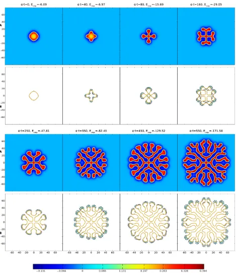
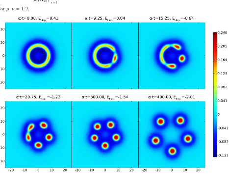
can pattern cortex with intricate structures. In Fig. 1A we show results of a direct numerical simulation
with a classic Mexican-hat choice forw. For further details see the discussion around equation (20) and
Appendix A.1 (for the numerical scheme). Here equation (1) describes a single population model with
short-range excitation and long-range inhibition. This minimal example nicely illustrates the ability of
neural field models to generate intricate spreading labyrinthine patterns. We do not expect to find
labyrinthine patterns as such in real brain activity. However, they provide a convenient (and visually
striking) proxy for the generation of complex patterns of activity, that emerge spontaneously and/or can be
evoked, for example in visual cortex [8]. Labyrinthine patterns are also seen when the Heaviside firing rate
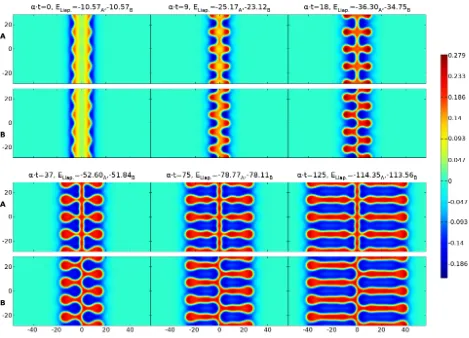
Figure 1: Labyrinthine structure emerging from (1) and (20) with parametersβ= 0.5,γ= 4 and Heaviside thresholdh= 0.115. The initial spot of radiusR= 12 has a mode four instablity, cf. Fig. 4. This is primed by perturbing R with 0.5 cos(4θ). Rows A show uand the colorbar below indicates its values. Rows B
illustrate the evolution of the interface (u=h, golden outline) due to the normal velocity of the boundary (green arrows, to scale but enlarged by a factor 50). The Liapunov functionELiap.of (2) is noted at all eight
the behavior of such patterns can be described simply by tracking the boundary between high and low
states of activity. Indeed this appears to resonate with neuroscientific practice, where changes of brain
activity are often of greater interest than the current brain state per se [9]. Hence it is of interest whether
the dynamics of (1) can be replaced by a lower dimensional description that evolves the boundary between
high and low states of activity. This programme has already been developed by Amari in his seminal paper
on one-dimensional models [10], where this interface reduces naturally to a point (or a set of points).
However, in two spatial dimensions the interface is more naturally a closed curve (or a set of closed curves).
The main topic of this paper is the development of an equivalent interface description for neural field
models of the type exemplified by (1). We show that activity patterns can be described by dynamical
equations of reduced dimension, and that these depend only on the shape of the interface (requiring no
knowledge of activity away from the interface). Not only is this description amenable to fast numerical
simulation strategies, it allows for the construction of localized states and an analysis of their linear
stability. Given the computational overheads in simulating the full neural field model this enhances our
ability to study pattern formation and suggests more generally that modeling the interfaces of patterns,
rather than the patterns themselves, may lead to novel, efficient descriptions of brain activity. Indeed the
use of interface dynamics to analyze patterns that arise in partial differential equation models of chemical
and physical systems has a strong history [11], and it is natural to translate some of the ideas and
technologies from these studies to non-local neural field models. The work by Goldstein [12, 13] and
Muratov [14] on pattern formation in two-dimensional excitable reaction-diffusion systems is especially
relevant in this context, as both authors have developed effective descriptions of interface dynamics in
terms of nonlocal interactions. See also the book by Desai and Kapral for a recent overview [15].
It is worth pointing out that whether computing interface dynamics can compete with other numerical
schemes will depend on the problem at hand. In general, boundaries that remain relatively short and do
not pinch guarantee a speed advantage. In practice, we expect this approach to be especially relevant for
(semi-) analytical work aiming at qualitative understanding, as illustrated by some of the examples
presented in this paper.
In§2 we present some of the key ideas behind an interface dynamics in the setting of a one-dimensional
neural field model. This is particularly useful for introducing the definition of normal velocity from a
level-set condition, as well as establishing what it means for an interface to be linearly stable. The
extension of these ideas to two-dimensional systems is presented in§3. By writing the synaptic
can be constructed in terms of line-integrals along the interface, and that the normal velocity of the
interface is driven by Biot-Savart-style interactions. Thus we obtain a reduced description for the evolution
of a pattern boundary solely in terms of quantities on the boundary itself. Numerical simulations of the
interface dynamics are shown to be in direct correspondence with those of the full neural field model. The
notion of linear stability of stationary solutions in the interface framework is fleshed out in a series of
examples (for spots, rings, stripes and fronts) in§4 and§5, and allows us to understand some of the
mechanisms for pattern formation. In§6 we add linear adaptation to (1) and extend our analysis to cover
this important neural phenomenon. This can introduce dynamic instabilities of stationary structures, and
we calculate where breathing and drift instabilities for localized spots occur. Moreover, we use a
perturbation argument to determine the shape of traveling spots that emerge beyond a drift instability and
show that spots contract in the direction of propagation and widen in the orthogonal direction. Finally, in
§7 we discuss extensions of the work in this paper.
2
A one-dimensional primer
Before we develop the machinery for describing the evolution of interfaces in two-dimensional neural field
models, it is informative to begin with a discussion in one dimension. In this case a minimal model can be
written in the form
ut=−u+ψ, ψ(x, t) =
Z
R
w(x−y)H(u(y, t)−h)dy, (3)
whereu=u(x, t) andx∈R,t∈R+. For a symmetric choice of synaptic kernelw(x) =w(|x|), which
decays exponentially, the one-dimensional model (3) is known to support a traveling front solution [16, 17]
that connects a high activity state to a low activity state. In this case it is natural to define a pattern
boundary as the interface between these two states. Thus we can define a moving interface (level set)
according to
u(x0(t), t) = const. (4)
Here we are assuming that there is only one point on the interface, though in principle we could consider a
set of points. The functionx0=x0(t) gives the evolution of the interface. Since the high and low activity
states in the neural field model are naturally distinguished by determining whetheruis above or below the
firing threshold, we shall take the constant on the right hand side of (4) to beh(though other choices are
also possible). Differentiation of (4) gives an exact expression for the velocity of the interface in the form
˙
x0=−
ut ux
x=x
0(t)
We can now describe the properties of a front solution solely in terms of the behavior at the front edge
which separates high activity from low. To see this, let us assume that the front is such thatu(x, t)> h for
x < x0(t) andu(x, t)≤hforx≥x0(t). Then (3) reduces to
ut(x, t) =−u(x, t) +
Z ∞
x−x0(t)
w(y)dy. (6)
Introducingz=ux and differentiating (6) with respect toxgives
zt(x, t) =−z(x, t)−w(x−x0(t)). (7)
Integrating (7) from−∞tot (and dropping transients) yields
z(x, t) =−e−t
Z t
−∞
esw(x−x0(s))ds. (8)
We may now use the interface dynamics defined by (5) to study the speedc >0 of a front, defined by
˙
x0=c. In this casex0(t) =ct, where without loss of generality we setx0(0) = 0, and from (6) and (8) we
have that
ut|x=x
0(t)=−h+we(0), ux|x=x0(t)=−we(1/c)/c, (9)
where
e
w(λ) =
Z ∞
0
e−λsw(s)ds. (10)
Hence from (5) the speed of the front is given implicitly by the equation
h=we(0)−we(1/c). (11)
To determine stability of the traveling wave we consider a perturbation of the interface and an associated
perturbation ofu. Introducing the notationb·to denote perturbed quantities, to a first approximation we will set uxb |x=
b
x0(t)=ux|x=ct, and write xb0(t) =ct+δx0(t). The perturbation inucan be related to the
perturbation in the interface by noting that both the perturbed and unperturbed boundaries are defined by
the level set condition, so thatu(x0, t) =h=ub(bx0, t). Introducingδu(t) =u|x=ct−ub|x=bx0(t), we thus have
the condition thatδu(t) = 0 for allt. Integrating (6) and dropping transients gives
u(x, t) = e−t
Z t
−∞
dses
Z ∞
x−x0(s)
dyw(y), (12)
andbuis obtained from (12) by simply replacingx0bybx0. Using the above we find thatδuis given (to first
order inδx0) by
δu(t) = 1
c
Z ∞
0
This has solutions of the formδx0(t) = eλt, whereλis defined byE(λ) = 0, with
E(λ) = 1−we((1 +λ)/c) e
w(1/c) . (14)
A front is stable if Reλ <0.
As an example consider the choicew(x) = exp(−|x|/σ)/(2σ), for whichwe(λ) = (λ+ 1/σ)−1/(2σ). In this case the speed of the wave is given from (11) as
c=σ1−2h
2h , (15)
and
E(λ) = λ
1 +c/σ+λ. (16)
The equationE(λ) = 0 only has the solutionλ= 0. We also have thatE0(λ)>0, showing thatλ= 0 is a
simple eigenvalue. Hence, the traveling wave front for this example is neutrally stable.
Given this preliminary exposition of interface dynamics we are now ready to describe the extension to two
dimensions and to address the additional challenges that working in the plane gives rise to.
3
Interface dynamics in two dimensions
As in the one-dimensional case we will define pattern boundaries as the interface between low and high
states of neural activity. To be more precise we introduce the notationB(t) to denote the (compact) area
of activity whereu≥h. The boundary, or interface,∂B(t) is defined by the threshold crossing condition
u(x, t) =h. In this case the model defined by (1) takes the form
ut(x, t) =−u(x, t) +ψ(x, t), ψ(x, t) =
Z
B(t)
w(|x−x0|)dx0, (17)
and the Liapunov function can be written simply as
ELiap.[u] =−
1 2
Z
B(t) dx
Z
B(t)
dx0w(|x−x0|) +h
Z
B(t)
dx. (18)
Note thatB(t) does not have to be simply connected and can describe a union of many disjoint active
regions. However, for clarity of exposition we shall focus on describing the evolution of an interface that is
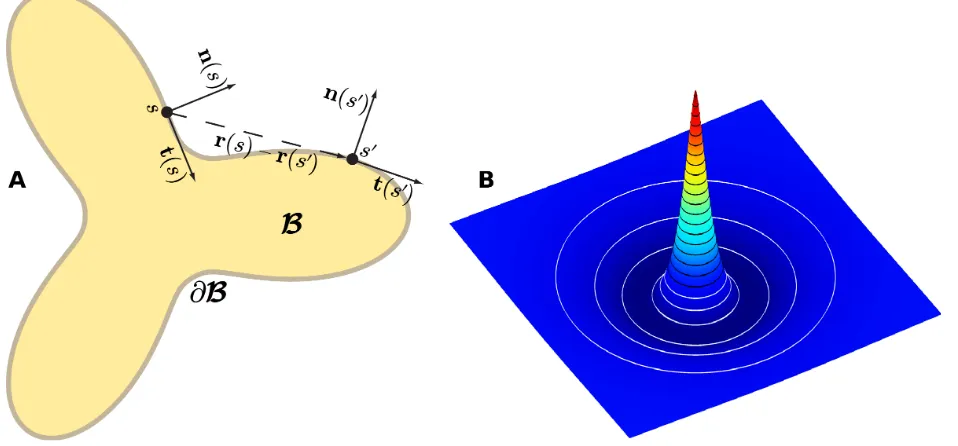
a single closed curve, as depicted in Fig. 2A. The extension to multiple closed curves is straight-forward.
It is well known that the two-dimensional model (17) can support localized states such as spots and
rings [18, 19] for a Mexican hat synaptic connectivity. Recent work in [6] has shown how to determine the
Figure 2: PanelA: Compact area Band boundary ∂B. Two points on the boundaryr, parametrized by s
ands0, are shown with their normalnand tangenttvectors. Panel B: Mexican hat (20) with parameters
β= 0.3 andγ= 3. White contours indicate values<0, black ones≥0, for a step size of 0.005.
numerical study for smooth sigmoidal firing rates can be found in [21]. These studies have highlighted, as
compared to the one-dimensional model, that an extra spatial dimension can lead to azimuthal instabilities,
whereby localized states can deform (or even split) into patterns with a reduced symmetry predicted by the
shape of the most unstable eigenmode. Direct numerical simulations beyond such instability points have
further shown the emergence of intricate spreading labyrinthine patterns like those in Fig. 1, that leave
behind a stable patterned state in their wake. It is our intention here to recover the Evans function results
for stability, albeit using a purely interface description of dynamics, as well as to determine the nonlinear
equations of motion that govern the evolution of labyrinthine (and other) structures. Moreover, by
employing a representation of the synaptic connectivity in terms of a linear combination of Bessel
functions, we can obtain an exact, though spatially reduced, dynamical system to describe the interface
that depends solely on the shape of the interface itself. In the following, we consider kernels of the form [3]
w(r) =
N
X
i=1
AiK0(αir), Ai∈R, αi >0, (19)
Mexican hat shape obtained from
w(r) = 2 3π
K0(r)−K0(2r)− 1
γ
K0(βr)−K0(2βr)
, β, γ >0, (20)
which is shown forβ= 0.3 andγ= 3 in Fig. 2B.
In an identical fashion to the way we derived an interface dynamics in one dimension in§2, we differentiate
u(x, t) =halong the contour∂B(t) to obtain
∇xu·
dr
dt + ∂u
∂t = 0, (21)
whereris a point on the domain boundary ∂B andut and∇xuare evaluated on the boundary.
Introducing the normal vector along the contour∂Bas n=−∇xu/|∇xu|allows us to obtain the normal
velocity along the contour:
n·dr
dt = ut
|z|. (22)
wherez≡ ∇xu(x, t)|x=r. Using (17) we see thatuandz satisfy
ut=−h+
Z
B
dx0w(|r−x0|), (23)
zt=−z+∇x
Z
B
dx0w(|x−x0|)
x=r
. (24)
From the form of (22), (23) and (24), we see that the evolution of the interface does not require any
knowledge of the neural field away from the contour, and rather just depends on the shape of the sets
where the field is above threshold. We now exploit the choice ofK0 as basis function for constructing the
synaptic kernel to show how the double integrals in (23) and (24) can be reduced to line integrals. This
yields an elegant description of the interface dynamics that emphasizes how the geometry of∂B drives the
evolution of spatiotemporal patterns. The key step in this reformulation is the use of Green’s identity. For
a two-dimensional vector fieldFthis identity is the two-dimensional version of the divergence theorem,
which we write symbolically asRB∇ ·F=H∂BF·n. Using this first identity we may generate a second for a scalar field Ψ asRB∇Ψ =H∂BnΨ.
To evaluate the right hand side of (23) and (24) it is enough to calculateR
Bdx0K0(α|x−x0|) and its gradient. In fact, this latter term can easily be rewritten as a line integral, using the second Green’s
identity, for any choice of synaptic kernel
Z
B
dx0∇xw(|x−x0|) =−
Z
B
dx0∇x0w(|x−x0|) =−
I
∂B
Using the fact thatK0(αx) satisfies the identityK0(αx) =α−2∇2K0(αx) + 2πδ(αx), as well as
∇xw(|x|) =w0(|x|)x/|x| andK00 =−K1, an application of Green’s first identity shows that
Z
B
dx0K0(α|x−x0|) = 1
α2
Z
B
dx0∇2xK0(α|x−x0|) + 2π
Z
B
dx0δ(α|x−x0|)
=−1
α
I
∂B
dsn(s)· x−r(s)
|x−r(s)|K1(α|x−r(s)|) +C
2π
α2. (26)
HereC= 1 ifxis withinBandC= 0 ifxis outsideB. Ifxis on the boundary ofBthenC= 1/2. Hence,
for points on the boundary parametrized bysone finds
ut(s) =−h+
N X i=1 Ai I ∂B
ds0n(s0)·Ri(s, s0) + π
α2
i
, (27)
zt(s) =−z(s)−
I
∂B
ds0n(s0)w(|r(s)−r(s0)|), (28)
where
Ri(s, s0) =−1
αi
r(s)−r(s0)
|r(s)−r(s0)|K1(αi|r(s)−r(s
0)|). (29)
Note that the choice ofK0 as a basis forwis merely a convenience to allow explicit calculations. As long
as we can write the connectivity functionwas the divergence of a vector field then we can exploit Green’s
first identity to turn the right hand side of (23) into a line integral.
From the Biot-Savart form of (29) we see that for every partiof the synaptic kernel there is an effective
repulsion between two arc length positions with anti-parallel tangent vectors, although the combined effect
when including allN terms will depend on the choice of the amplitudesAi. Now with (22), (27) and (28)
the normal velocity on the interface can be written solely in terms of certain line-integrals around the
interface. From a computational perspective this leads to a substantial advantage in that one no longer
needs to solve the full non-local neural field model (17) across the entire plane, and can instead simply
evolve the interface in time by discretizing the boundary and translating the points with the normal
velocity from (22) in the direction ofn. One possible practical disadvantage of this is the need to monitor
for possible self-intersections of the evolving boundary,splitting, where a connected region pinches off into
two or more disconnected regions, or indeed the creation of new boundaries where none existed before.
However, numerical schemes for coping with similar situations in fluid models are well developed in the
literature and it is natural to turn to these for more refined numerical schemes and ones that can automate
the process of contour surgery [22, 23]. In Fig. 1B we illustrate the simple numerical implementation of the
interface dynamics described in Appendix A.2, showing the effectiveness of the dimensionally reduced
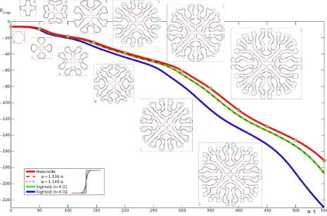
Furthermore, in our calculations we have found that the key assumption of a Heaviside firing rateH(u−h)
can be relaxed to a degree without fundamentally changing the results. This is illustrated in Fig. 3, where
we show the evolution in time of theu=hinterface and the corresponding Liapunov function. The
evolution with a Heaviside firing rateH(u−h) is shown in red, and compared with simulations of the full
neural field model using more biologically realistic sigmoids 1/{1 + exp[−(u−h)/σ]}, withσ= 0.01 in
green andσ= 0.02 in blue. Hereσ reflects the expected width of the distribution of firing thresholds
around a meanhin the neural population, with the Heaviside case corresponding toσ= 0. Fig. 3
demonstrates that for these steep sigmoids very similar labyrinthine shapes arise, and closer inspection
reveals that the main differences occur at the rapidly developing rim of the structure, whereas the settled
interior is nearly identical. Thus a simple adjustment of the time constantαwill in this case provide a near
perfect match of the emerging structures. In Fig. 3 we demonstrate this with the dashed and dotted red
lines, which represent the Heaviside Liapunov function computed over longer time scales (up to
α·t= 569.9 and 626.8, respectively) and then scaled down toα·t≤550 by adjustingα. A very close
match to the sigmoidal Liapunov curves (green and blue lines) is then obtained. However, for broader
sigmoids we find labyrinths still resembling the Heaviside one, but with more obvious spatial changes. The
supplementary Video S3 shows theσ= 0.03 case as an example. It would seem that mild deviations in the
shape of the firing rate from Heaviside (to a steep sigmoidal form) are reflected more in temporal speed
than in spatial shape changes.
The Liapunov function can also be written in terms of line integrals: ELiap.= 1/2P N
i=1AiFi+hΓ, with
Fi= 1
α2 i I ∂B ds I ∂B
ds0t(s)·t(s0)K0(αi|r(s)−r(s0)|)− 2π α2
i
Γ, (30)
where Γ =RBdxis the area of the domain above threshold andt(s) = dr(s)/dsis the tangent vector, which can also be constructed fromnby an anti-clockwise rotation ofπ/2 so that
n=
0 1
−1 0
t. (31)
To obtain (30) we have used the fact that
Z
B
dx
Z
B
dx0K0(α|x−x0|)− 2π α2Γ =−
1
α2
Z
B
dx∇x·
Z
B
dx0∇x0K0(α|x−x0|)
=− 1
α2
Z
B
dx∇x·
I
∂B
ds0n(s0)K0(α|x−r(s0)|)
=− 1
α2 I ∂B ds I ∂B
ds0n(s)·n(s0)K0(α|r(s)−r(s0)|), (32)
As well as providing a computationally useful framework for studying pattern formation, the interface
dynamics including its Liapunov function is also amenable to a direct linear stability analysis. This is
especially useful for understanding how the instability of localized stationary states can seed interesting
structures, like the labyrinths of Figs. 1 and 3. Stationarity of a solution means that the normal velocity is
zero all along the boundary of the active area. This is equivalent to demandingut= 0 on the boundary. In
this case (22) reduces to
h=
Z
B0
dx0w(|r−x0|) =
N
X
i=1
Ai
I
∂B0
ds0n(s0)·Ri(s, s0) + π α2
i
, (33)
whereris on the boundary parametrized bys. We use the notationB0 to denote a stationary active
region. Given the stationary interface, we can also calculate the stationary fieldueverywhere (away from
the interface) using (17) as
u(x) =
Z
B0
dx0w(|x−x0|), (34)
which can also be evaluated as a line integral. In order to analyze the stability of stationary solutions in
the original neural field formalism defined by (1) one would perturb the field variableuand linearize to
derive an eigenvalue equation or Evans function [20]. Here we determine stability using the interface
dynamics, generalizing the approach described in§2.
Using the notationb·again to denote perturbed quantities, we consider small perturbations to the contour shape and denote the new interface by∂cB. The relationship between the perturbed interface and the
perturbed field is, as in one dimension, determined by the conditionδu(t) = 0, where
δu(t) =ub|x∈
c
∂B−u|x∈∂B0. (35)
The dynamics forubis given by (23) withBreplaced byBb. The perturbation affects the normal vectorn(s)
as well as the displacement vectorr(s)−r(s0) that occurs in (27). Thus to evaluate (35) it is necessary to
linearizeK1about the unperturbed contour. In the case of interfaces without curvature the linear
contribution toK1 is zero. In contrast for curved interfaces an addition theorem for Bessel functions shows
that there is a non-zero contribution. To clarify this statement and show how the above machinery is used
in practice, we now give some explicit examples of localized solutions and their stability.
4
Localized states – spots
We consider spots to be circular stationary solutions. They are the equivalent of the bumps known in one
spatial dimensions they can undergoazimuthal instabilities, as already found in [6]. In order to obtain
circular solutions we use the standard parametrization of a circle for the contour and write
r(θ) =R
sinθ
1−cosθ
, n(θ) =
sinθ
−cosθ
, θ∈[0,2π). (36)
Hence the right hand side of (33) can be calculated using
I
∂B
ds0n(s0)·Ri(s, s0) = 1
αi
Z 2π
0
dθK1[αiR(θ)]
R(θ) R(1−cosθ), (37)
whereR(θ) =Rp2(1−cosθ). Using Graf’s formula [24] to perform the integration in (37) we obtain an implicit equation for the spot radiusR in the form
h= 2π N X i=1 Ai 1 α2 i − R αi
K1(αiR)I0(αiR)
, (38)
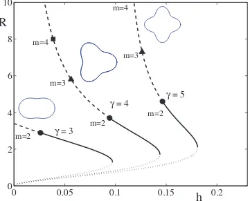
whereIν(x) is the modified Bessel function of the first kind of orderν. A plot of the spot radiusR as a
function of thresholdhis shown in Fig. 4.
To determine the relationship between a perturbed and unperturbed spot we need to examine the
conditionδu(t) = 0. The general solution foru(dropping transients) can be written as
u(x, t) = e−t
Z t
−∞
dsesψ(x, s). (39)
For a circular solution of radiusR ψ is conveniently written as
ψ(r) =
Z 2π
0
Z R
0
w(|r−r0|)r0dr0dθ, r= (r, θ). (40)
Hereψ may be constructed explicitly (off the boundary), using similar line integral calculations to those
for existence (above), and is given explicitly by
ψ(r) = 2πR N
X
i=1
AiLi(r), (41)
where
Li(r) =
( 1
αiI1(αiR)K0(αir) r≥R
1
α2
iR
− 1
αiI0(αir)K1(αiR) r < R
. (42)
For perturbations in the radius of the formRb=R+δR(θ, t) one finds
δu(t) =
Z ∞
0
dse−s
Z 2π
0 dθ0
(
Z Rb(θ0,t−s)
0
w(|r−r0|)|r=(
b R(θ,t),θ)r
0dr0−Z
R
0
w(|r−r0|)|r=(R,θ)r0dr0
)
=
Z ∞
0
dse−s
Z 2π
0
0
0.05
0.1
0.15
0.2
0
2
4
6
8
10
h
R
γ
= 3
γ
= 4
γ
= 5
m=2
m=2
m=3
m=4
m=2
m=3
[image:15.612.132.493.237.528.2]m=4
Using the above we see thatδu(t) = 0 has solutions of the formδR(θ, t) = cosmθeλmt, where
λm=−1 +Wm, (44)
and
Wm= R
|ψ0(R)|
Z 2π
0
dθcos(mθ)w(R(θ)) =
PN
i=1AiKm(αiR)Im(αiR)
PN
i=1AiK1(αiR)I1(αiR)
. (45)
Note that sinceWm is realλm∈R. A mode-minstability will occur ifλm>0, which recovers the result
in [6] obtained using an Evans function approach. The possibility of such azimuthal instabilities is
indicated on the solution branches shown in Fig. 4 (and we would expect the emergence of solution
branches withDm symmetry from the points marked bym). Interestingly we can see from (44) and (45)
that the mode withm= 1 is neutrally stable. For a perturbation to a circular boundary of the form
δR(θ, t) =m(t) cos(mθ),m=eλmtand1, the perturbation of the normal velocityvn is
vn=mcos(mθ)(−1 +Wm). (46)
To calculate the Liapunov function for an unperturbed spot we evaluate (30) using
1
α2
i
Z 2π
0 dθ
Z 2π
0
dθ0R2cos(θ−θ0)K0(αiR(θ−θ0)) = 2π2
α2
i
R2K1(αiR)I1(αiR)≡Gi. (47)
Hence
ELiap.=
1 2 N X i=1 Ai
Gi−
2π α2
i πR2
+hπR2 (48)
The zeros of the first derivative ofELiap.with respect toR give the stationary circular solutions, including
the trivial caseR= 0, as expected.
5
Rings, fronts and stripes
In this section we show how to treat other simple interface shapes, namely rings, fronts and stripes, and
determine their stability. We recover previous results in [6] for rings (obtained with an Evans function
method), whilst calculations for the other structures are shown to be straight-forward using the interface
dynamics approach.
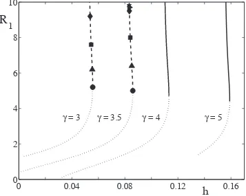
5.1 Rings
Rings can be considered as the difference of two spots, one with radiusR1and the other with radius
R2> R1. Introducingψ(r, R) = 2πRPiAiLi(r, R), where Li(r, R) is given by the right hand side of (41),
0
0.04
0.08
0.12
0.16
0
2
4
6
8
10
h
R
1
[image:17.612.136.493.240.525.2]γ
= 3
γ
= 3.5
γ
= 4
γ
= 5
pair of equations that determine (R1, R2). To establish stability the outer contour is perturbed exactly as
in the previous section: R2(θ) =R2+aeλtcosmθ, for some small amplitudea. For the inner contour we
similarly writeR1(θ) =R1+beλtcosmθ. We now generate δu(t) on each of the two boundaries and equate
these to zero to generate two equations for the pair of unknown amplitudes (a, b). Demanding that this
pair of equations has a non-trivial solution generates an equation forλin the formEm(λ) = 0 where
Em(λ) =|(1 +λ)I2− Am(λ)|and
[Am(λ)]µν = Rν
|u0(Rν)|
Z 2π
0
dθcos(mθ)wqR2
µ+R2ν−2RµRνcosθ
= Rν
|u0(Rν)|
N
X
i=1
Ai[Km(αiRµ)Im(αiRν)H(Rµ−Rν) +Km(αiRν)Im(αiRµ)H(Rν−Rµ)], (49)
[image:18.612.74.541.280.635.2]forµ, ν= 1,2.
Figure 6: Direct numerical simulation of u for a ring solution (R1 = 7, R2 = 8.629) perturbed with a linear combination of modes 0,1,2, . . . ,8. For the given parametersβ = 0.5,γ= 3 and Heaviside threshold
h= 0.0549, modem= 5 is most unstable, cf. Fig. 5. See also the supplementary Video S4.
-0.2
-0.1
0
0.1
0
0.2
0.4
0.6
0.8
1
λ
k
varicose
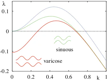
[image:19.612.119.493.107.390.2]sinuous
Figure 7: Spectra for the Mexican-hat function (20) with β = 1/2 andγ = 4: for a stationary front (blue line, 2h= 1−1/(γβ2)), and varicose (green line) and sinuous (red line) stripes of widthD= 7, respectively.
solution branches for ring solutions as a function ofhfor the Mexican hat model defined by (20), and flag
the types of instability that can occur. Of the two solution branches the lower one is unstable with respect
to radial perturbations, whereas the upper branch is subject to azimuthal destabilizations. In Fig. 6 we
show a two-dimensional plot of an unstable ring solution, and the emergent structure of five bumps seen
beyond instability, consistent with the predictions of our linear stability analysis.
5.2 Fronts
Calculating stationary planar fronts is straightforward, since the normal vectorn(s) is orthogonal to the
displacement vectorr(s)−r(s0) and the line integral on the right hand side of (33) is zero. Hence we have
the existence conditionh=P
iAiπ/α
2
i and we note thathlies exactly halfway between the two possible
treat the simple casew(x) =K0(x)/(2π). We then have thatut=−h+ 1/2 and
|z|=
Z ∞
0
dse−s
Z ∞
−∞
dy 1
2πK0(
p
y2+ (cs)2) = 1 2
1
1 +c, c >0. (50)
Hence using (22), the normal velocity is given by
c= 1−2h
2h . (51)
To determine stability we consider a front alongy= 0 and write the perturbed front asyb=yb(x, t). For simplicity we shall focus on a stationary front withc= 0. In this case we may constructδu(t) as
δu(t) =
Z ∞
0
dse−s
Z ∞
−∞
dx0[yb(x, t)−yb(x0−x, t−s)]w(x0). (52)
The equationδu(t) = 0 (for allx) has solutions of the formby=cos(kx)eλt, where
λ=−1 +wb(k) b
w(0), wb(k) = Z ∞
−∞
dx w(x) cos(kx). (53)
For a modified Bessel function one has
Z ∞
−∞
dx K0(αx) cos(kx) = 1
√
α2+k2. (54)
Hence for the simple example above, the stationary planar front is stable due towb(k)≤wb(0). However, for a Mexican hat function it is possible thatwb(k)>wb(0) for some band of wave numbers, and we would expect instabilities in this case. Figure 7 showsλ=λ(k) for a stationary front with the Mexican-hat
function (20), from which the critical band of wave numbers can easily be read off.
It is also possible to calculate the properties of circular fronts. For such fronts (really spots) with a small
radiusR, we may use the approximation that K1(x)'1/xto evaluate (37) as follows
I
∂B
ds0n(s0)·Ri(s, s0)' π α2
i
1
R. (55)
The normal velocity can be calculated from (22) and written in the form
dR
dt =
1
|z|
"
−h+
1 + 1
R
X
i Aiπ
α2
i
#
. (56)
IfP
iAiπ/α2i ≥h, thenR(t) will increase and the solution may approach a planar front – if this solution is
stable, see above. IfP
iAiπ/α
2
i < hthen there is a unique stationary spot, which is unstable for
P
iAiπ/α
2
collapse
collapse
sinuous &
sinuous &
varicose
varicose
Γ=
3
Γ=
3
Γ=
4
Γ=
4
Γ=
5
Γ=
5
[image:21.612.117.493.109.357.2]0.00
0.05
0.10
0.15
0.20
0
2
4
6
8
10
h
D
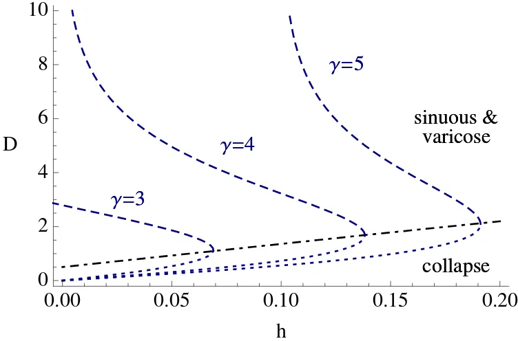
Figure 8: Stripe widthsDfor different values ofγwith a Mexican hat interaction given by (20) andβ = 0.5.
5.3 Stripes
A stripe may be considered as the active area in between two interacting stationary fronts. For two
interfaces that define a stripe to be alongy=y1 andy=y2, then
u(x, y) =
Z ∞
−∞
dx0
Z y2−y
y1−y
dy0w(p(x0)2+ (y0)2). (57)
For a strip of constant widthD, such thaty2−y1=D for allx, the existence condition
u(x, y1) =h=u(x, y1+D) takes the simple form
h= Z ∞ −∞ dx Z D 0
dyw(px2+y2) =X
i Aiπ
α2
i
1−e−αiD
. (58)
An example ofD=D(h) is shown in Fig. 8 for a Mexican hat function.
To determine stability we consider perturbations on each of the two stripe boundaries and constructδui on
each as
δui(t) =
Z ∞
0
dse−s
Z ∞
−∞
dx0
( Z by1(x
0−x,t−s)−
b yi(x,t)
b
y2(x0−x,t−s)−byi(x,t)
−
Z D
0
)
dy0w(p(x0)2+ (y0)2), (59)
fori= 1,2. When considering small perturbations there is some ambiguity in expanding (59) depending on
Figure 9: Direct numerical simulation ofufor varicose (rowsA) and sinuous (rowsB) instabilities±cos(ky) with k = 0.44272 of a stripe of width D = 7 for parameters β = 0.5, γ = 4.0 and Heaviside threshold
which means that we may expand (59) to obtain
δui(t) =
Z ∞
0
dse−s
Z ∞
−∞
dx0w(p(x0)2+D2)[
b
y2(x0−x, t−s)−yib(x, t)]
±
Z ∞
0
dse−s
Z ∞
−∞
dx0w(x0)[by1(x0−x, t−s)−yib(x, t)]. (60)
The equationsδui = 0 admit solutions of the formyib =yi+icos(kx)eλt. For equal amplitude perturbations,|1|=|2|=, there are two branches of eigenvalues given byλ=λ±, where
λ±=−1 +
F±(k, D)
F+(0, D)
. (61)
HereF±(k, D) =wb(k,0)∓wb(k, D) and
b
w(k, D) =
Z ∞
−∞
dx w(px2+D2) cos(kx) =X
i Aie
−D√α2
i+k2
p
α2
i +k2
. (62)
The branch withλ=λ+corresponds to sinuous perturbations with (1, 2) =(1,1) and the branch with
λ=λ− corresponds to varicose perturbations with (1, 2) =(1,−1). Sinceλ+> λ− then sinuous
instabilities dominate over varicose. Note that asD→ ∞we recover the existence and stability results for
a stationary front as expected. Examples of sinuous and varicose instabilities (as predicted from our
analysis) are shown in Fig. 9.
6
Neural field models with linear adaptation
In real cortical tissues there are an abundance of metabolic processes whose combined effect is to modulate
neuronal response. It is convenient to think of these processes in terms of local feedback mechanisms that
modulate synaptic currents. For example, it is known that a model of synaptic depression can destabilize a
spot in favor of a traveling pulse [25]. Here we consider a simple linear model of adaptation that is known
to lead to instabilities of localized structures [26]. In this case the original neural field model is modified
according to
1
αut=−u+ψ−ga, at=u−a, (63)
withg >0. Hereψis the second term on the right hand side of (3) and (1) in one and two dimensions,
respectively. The linearity of the equations of motion means that we may obtain the trajectory for (u, a) in
closed form as
u(·, t) =
Z t
−∞
dsη(t−s)ψ(·, s), a(·, t) =
Z t
−∞
dse−(t−s)u(·, s), (64)
where
η(t) = α
λ−−λ+
Here
λ±=
1 +α±p(1 +α)2−4α(1 +g)
2 . (66)
As an example let us compute the speed (c >0) and stability of a front in the one-dimensional model
discussed in§2 with the inclusion of a linear adaptation current. In this case we have that
ut|x=x0(t)=ch/σ, (67)
ux|x=x
0(t)=−
1
c
Z ∞
0
dsη(s/c)w(s)
=− α
c(λ−−λ+)
[(1−λ+)we(λ+/c)−(1−λ−)we(λ−/c)]. (68)
Note that to calculateutwe have used the result thath=u(ct, t) =R0∞dsη(s)Rcs∞dyw(y). Hence, from (5), the speed is determined implicitly by
h= α 2
c/σ+ 1 (c/σ+λ+)(c/σ+λ−)
, (69)
which may be rearranged to give
c σ =−
1 2
"
1 +α− α
2h±
s
1 +α− α
2h
2
−4α
1 +g− 1
2h
#
. (70)
The eigenvalue equation for stability can also be calculated, generalizing the analysis of§2, as
E(λ) = 1− H(λ)/H(0), where
H(λ) = α
λ−−λ+
{(1−λ+)we((λ+λ+)/c)−(1−λ−)we((λ+λ−)/c)}. (71)
On the branch withc= 0 where 2h(1 +g) = 1, defining a stationary front, we find that
E(λ) =λ(λ+λ++λ−−λ+λ−)
(λ+λ+)(λ+λ−)
, (72)
which has zeros whenλ= 0 andλ=k+k−−(k++k−) =αg−1. Hence, the stationary front changes from
stable to unstable asαis increased through αc = 1/g.
In two-dimensions it is straight forward to construct a stationary spot of radiusR. This radius is
determined by (38) under the replacementh→h(1 +g), so that
h(1 +g) = 2πR N
X
i=1
AiK0(αiR)I1(αiR)/αi ≡F(R). (73)
Hereψ may be constructed explicitly off the boundary, and is given by equation (41), so that
Hence, in the (h, g) plane stationary solutions only exist for h < F(Rc)/(1 +g). Under variation inαwe
expect the emergence of a drifting spot. Beyond a drift instability, we expect to be able to find traveling
spots that move in some directioncwith constant speedc=|c|. These can be constructed as stationary
solutions in a co-moving frameξ=x+ct, and satisfy
1
αc· ∇ξu=−u+ψ−ga, c· ∇ξa=u−a. (74)
We may write the velocity in terms of local co-ordinates on the moving interface asc=cnn+ctt, where
cn(s) =c·n(s) is the normal velocity andct(s) =c·t(s) the tangential velocity at a point on the interface.
Taking the cross product ofcandt(and usingn×t= 1) shows that cn=c×t. Hence, the condition for
stationary propagation, withc= ˙r, is
n(s)·r˙(s) =c×dr(s)
ds
dr(s) ds
, u(ξ)|ξ=r=h. (75)
In general this is a hard equation to solve in closed form. However, to obtain an estimate of the speed and
shape of a spot beyond a point of instability it is enough to consider a weak distortion of a traveling
circular wave [27]. Choosingc=c(1,0) and writingξ= (ξ1, ξ2), and assuming thatψis rotationally
symmetric means that we may construct a solution in the form
u(ξ1, ξ2) = 1
c
Z ξ1
−∞
dyη((ξ1−y)/c)ψ
q
y2+ξ2 2
. (76)
We note that the threshold conditionu=hfor a circular spot (ξ2
1+ξ22=R2) can only strictly be met for
the casec= 0, since the right hand side of (76) depends on the plane polar angle throughξ1=Rcosθ. For
this case we may construct the equationδu(t) = 0 to determine the eigenvaluesλmthat occur in
perturbations of the formδR(θ, t) =eλmtcos(mθ) as solutions toE
m(λ) = 0, where
Em(λ) =
1
e
η(λ)−(1 +g)Wm, (77)
whereWm is given by (44) and the Laplace transform ofη is easily calculated as
e
η(λ) = α(1 +λ) (λ+λ+)(λ+λ−)
. (78)
The eigenvalues form= 1 are determined byηe(λ) = 1/(1 +g), which has two solutions: λ= 0 and
λ=αg−1. Hence this mode becomes unstable asg increase through 1/α. It is also possible that a
breathing instability may arise for the mode withm= 0. Note that another way to generate breathing
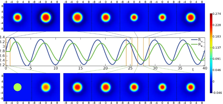
Figure 10: Breathing instability from direct numerical simulation with parametersα= 5, β = 0.5,γ = 4, coupling strength g = 0.5 and Heaviside threshold h= 0.12/(1 +g). Initial data was constructed from a stationary spot solution by modifying the adaptation variable to a top-hat shape. Top and bottom rows: snapshots of activation u and adaptation a, respectively, at times indicated by orange lines in the middle row. Middle row: above threshold radii as function of time. See also the supplementary Video S6.
Substitution ofλ=iω into (77) gives the condition for this instability as:
W0= 1 +α
α(1 +g), g≥ 1
α, (79)
with emergent frequencyω=√αg−1. Form≥2 splitting instabilities can be determined by setting
λ= 0 in (77) to give the conditionsWm= 1. An example of a breather arising as an instability of a spot is
shown in Fig. 10 (and numerical simulations confirm the predicted value of the emergent frequency around
the bifurcation point).
Anticipating a smallcdiscussion we Laplace transform (76) in the ξ1 variable to obtain
e
u(λ, ξ2) = 1 1 +g
1 + 1
α(1 +g)[(αg−1)cλ−α(cλ)
2+ (cλ)3+. . .]
e
ψ(λ, ξ2), (80)
which we then inverse transform to obtain
u(ξ1, ξ2) = 1 1 +g
1 + 1
α(1 +g)[c(αg−1)
∂ ∂ξ1
−αc2 ∂
2
∂ξ2 1
+c3 ∂
3
∂ξ3 1
+. . .
ψ(|ξ|). (81)
At the point whereg= 1/α, the shape of the spot deviates from circular with an amplitude that depends
drifting instability to a traveling spot whose shape, determined from (81) byu(r) =h, can be written in
the formr(θ) =R(θ)(cosθ,sinθ) with
R(θ) =R+X
m≥2
cmamcosmθ. (82)
HereR is determined by (73). A further weakly nonlinear analysis to understand the competition between
drifting and breathing atg= 1/αis beyond the scope of this paper.
Forg >1/αand dropping terms ofO(c2) in (81) we see that there are solutions tou(r) =hof the form
R(θ) =R+a1ccosθ, wherea1= (1−αg)/(α(1 +g)2)<0. The amplitudes of higher order modes may be
constructed in a similar fashion, i.e., by balancing terms at each order inc inu(r) =husing (81) and (82).
However, it is not our intention to pursue these lengthy calculations here. Rather to give a feel of the shape
of a traveling spot we plot the level set whereu(ξ1, ξ2) =husing (81) in Fig. 11D including terms up toc3.
This nicely illustrates that spots contract in the direction of propagation and widen in the orthogonal
direction, and provides a theoretical explanation for the shape of traveling spots recently reported in [28].
With the aid of direct numerical simulations we have also explored the scattering properties of traveling
spots. In common with previous numerical studies of planar neural fields with some form of adaptation, we
find that such structures can behave as quasi-particles in the sense that they can scatter like dissipative
solitons [29]. An example of such scattering is shown in Fig. 11. Here we see a repulsive interaction which
repels the spots away from each other if they approach too closely.
7
Discussion
In this paper we have formulated an interface dynamics for planar neural fields with a Heaviside firing rate.
This has allowed us to i) develop an economical computational framework for the evolution of
spatiotemporal patterns, and ii) perform linear stability analyses of localized structures. For simplicity we
have focused on single population models. However, the extension to population models that treat the
dynamics of both excitatory and inhibitory populations is straightforward. Perhaps a more interesting
extension is to consider neural field models that incorporate feature selectivity such as that observed in
visual cortex for orientation [30], spatial frequency [31] and texture [32]. Denoting this feature label byχ
then all of these models are expressed in terms of some non-local integro-differential equation foru(r, χ, t).
We note that the notion of an interface is still well defined and that the level set conditionu(r, χ, t) =h
gives a constraint between local geometrical data and features. As an alternative to simulating the neural
Figure 11: Collision of two pulses from direct numerical simulation with parameters as in Fig. 10. Columns
local data can be integrated into global geometrical structures, as advocated in the neurogeometry
framework of Petitot [33] (say for understanding models of contour completion in models of primary visual
cortex where the feature space is orientation). The extension of this work to treat sigmoidal firing rates
remains an open challenge. However, recent techniques for dealing with a certain class of firing rate
functions in one spatial dimension, which includes smooth firing rate functions connecting zero to one, are
likely to be useful in this regard [34]. We have included an adaptive current in the standard Amari model
here, but it would be informative to develop interface treatments for other forms of modulation, e.g.,
arising from threshold accommodation [35] or synaptic depression [5], as well as the inclusion of axonal
delays [36]. These models can readily support spiral wave activity, and it would be interesting to see if an
interface description, possibly adapting techniques by Hagberg and Meron [37], could shed light on their
properties. Another possible extension of the work in this paper, motivated by our numerical results for
scattering spots, is to develop an interface theory of quasi-particle interactions along the lines for
reaction-diffusion models described in [38, 39], using ideas developed by Bressloff [40] and Venkov [41] for
weakly interacting systems in one spatial dimension. All of the above are topics of ongoing research and
will be reported upon elsewhere.
Supplementary material
Video S1. Emergence of a labyrinthine structure inuas shown in snapshots in Fig. 1. PanelsAandB
in the animation correspond to rowsAandBof that figure, and displayed content, parameters and
initial condition are discussed in its caption. The 120×120 domain was discretized by a 4096×4096
grid. Note that the Fourier technique used, see Appendix A.1, implies periodicity and turns the
domain effectively into a torus.
Video S2. In panelAthe values ofufrom three direct numerical simulations are overlaid by assigning
each one a part of the red-green-blue color space. The Heaviside model, cf. Fig. 1 and Video S1,
determines red intensity, whereas calculations with a sigmoidal firing rate 1/{1 + exp[−(u−h)/σ]},
cf. Fig. 3, determine intensities in green forσ= 0.01 and blue forσ= 0.02. Where all three models
predict thesamevalue foru, a gray color results as shown by the colorbar. Where the models predict
different values, colored patches show up. In panelBthe same data is displayed, but this time only
theu=hinterface is plotted with the same color assignment. From about timeα·t= 550 onward
Video S3. The same model as in Fig. 1 but with a sigmoidal firing rate 1/{1 + exp[−(u−h)/σ]}with
σ= 0.03. A comparison with the Heaviside model, Fig. 1 and Video S1, as well as the sigmoid model
with smallerσ, Fig. 3 and Video S2, shows that broadening the sigmoid eventually leads to
significant deviations from the Heaviside prediction. This illustrates the practical limits of the
interface method proposed in this paper.
Video S4. Decay of a perturbed ring solution inuinto five spots as shown in snapshots in Fig. 6.
Displayed content, parameters and initial condition are discussed in that figure’s caption. The
50×50 domain was discretized by a 2048×2048 grid. Note that the simulation time (displayed on
top of the uplot) is nonlinearly related to the actual play time of the animation, in order to capture
both the rapid structural change from ring to spots at the beginning and the slow drifting apart of
the spots that follows.
Video S5. Varicose and sinuous instabilities of a stripe as shown in snapshots in Fig. 9. PanelsAandB
in the animation correspond to rowsAandBof that figure, and displayed content, parameters and
initial condition are discussed in its caption. For the present set of parameters varicose instabilities
occur for 0.27< k <0.69, whereas sinuous instabilities occur for 0< k <0.69. The domain size is set
to 8π/k in the ordinate to guarantee that perturbations±cos(ky) are periodic. The domain size in
the abscissa is 16π/k and the domain was discretized by a 4096×2048 grid.
Video S6. Breathing spot as shown in snapshots in Fig. 10. PanelsAandB in the animation
correspond to the top and bottom row of that figure, and displayed content and parameters are
discussed in its caption. Both activationuand adaptationastart with radiusR= 2.8 above
threshold, the former with a spot solution and the latter with a disc of constant value 0.25g. The
spot oscillates with angular frequencyω= 1.1, close to the theoretical prediction from linear stability
analysis (ω=√αg−1'1.2, with increasing agreement as one approaches the bifurcation point
αg= 1 from above). The actual domain was 34×34, of which only part is shown, and was
discretized by a 1024×1024 grid.
Video S7. Collision of two travelling spots as shown in snapshots in Fig. 11. PanelsA-C in the
animation correspond to rowsA-Cof that figure, and displayed content and parameters are
discussed in its caption. Note that timet= 0 in the figure corresponds tot= 36.95 in the animation.
co-located discs inaof the same radius. The discs have a linear gradient along the abscissa from zero
to 0.5g, while having uniform values along the ordinate. The mean position of theu≥hregions of
the pulses is kept track of during time evolution and used to estimate the current velocities. The
34×34 domain was discretized by a 1024×1024 grid.
A
Numerical schemes
A.1 Fourier technique for neural field evolution
Because of its non-local character, the model described by (1), or its extension (63), is challenging to solve
with conventional numerical methods. However, exploiting the convolution structure of (1) allows one to
write the Fourier transform ofR
R2dx
0w(|x−x0|)f(x0, t) as a product. Heref(x, t) =H(u(x, t)−h) and
can be taken either as a Heaviside or a more general sigmoidal form. Introducing a spectral wave-vectork
then this product is simplyw(|k|)f(k), where functions with argumentskdenote two-dimensional spatial
Fourier transforms. We may evaluatew(|k|)f(k) directly, at every time step, using fast Fourier transforms
(FFTs). Note thatw(|k|) can be pre-computed, by FFT or here even analytically, so that the procedure
iterated over time amounts to computingf(k) by FFT, followed by a (complex) multiplication withw(|k|),
and finally an inverse FFT to obtain the result of the integral. We wish to employ a parallel compute
cluster for rapid computation over large grids, and hence use the free software package FFTW 3.3 [42],
which includes a parallel MPI-C version. Note that the use of Fourier methods implies that the
discretization grid has periodic boundaries, or in other words, the solution is effectively computed on a
torus. We use a grid spacing of about 0.03 or better in our computations here.
In order to compute the time evolution, we use DOPRI5 [43], a well-known implementation of an explicit
Dormand-Prince (Runge-Kutta) method of order 5(4) with step size control and dense output of the order
4. A version in C due to J. Colinge is available on the web thanks to E. Hairer. However, in our case we
perform parallel computations, so we have adapted this code accordingly using MPI-C. In particular, we
now consider the maximum error across all compute nodes and all variables, rather than the mean error
over local variables, and communicate the resulting time step adaptation over the cluster to achieve a
unified evolution of the entire distributed grid. Numerical tolerances are set to 10−7(|y
i|+ 1) whereyi
represents all variables, i.e.,uand potentiallyaat all grid points.
This numerical method is robust against effects of the underlying grid. This is due to the employed Fourier
method, which performs the spatial convolution as a multiplication in Fourier space. The discrete Fourier
polynomial, and the influence of the grid is effectively smoothed by implicit interpolation.
Computing an evolution as shown in Video S1 takes several hours on the 32 to 64 Infiniband-connected
compute nodes we have typically employed, and yields many gigabytes of data. We note that computation
with a sigmoidal firing rate instead of the Heaviside one is over an order of magnitude faster, reflecting the
numerical difficulty of dealing with sharp edges.
A.2 Interface dynamics
Equations (22) and (28) can be used to develop a numerical scheme. The contour∂Bis discretized into a
set of points, and the normal vectors and the displacement vectors are found by computing the orientation
and distance between points. Hence the computation of the contour integrals in (28) is straight-forward
and yields the normal velocity, cf. (22), which is used to displace the points of the contour in the normal
direction at every time step. We employed a simple Euler method to calculate the dynamics of the contour.
As the contour grows / shrinks, additional points have to be created / eliminated along the contour.
This method does not provide any means to deal with the splitting or emergence of contours. It is faster
than the Fourier technique (see Appendix A.1) for small contours, yet the time to compute the normal
velocity is proportional toN2 (N being the number of points discretizing the contour), as opposed to
M√M for the Fourier technique (whereM is the number of grid points). Hence it becomes slower for
larger contours due to the absence of suitable spectral methods to compute the line integrals. The main
advantage of this method is the fact that no underlying grid has to be deployed across the specified domain.
References
1. Coombes S:Large-scale neural dynamics: Simple and complex.NeuroImage2010,52:731–739. 2. Liley DTJ, Foster BL, Bojak I:Computational Systems Neurobiology, Springer,Volume to appear 2012 chap.
Co-operative populations of neurons: Mean field models of mesoscopic brain activity.
3. Folias SE, Bressloff PC:Breathing pulses in an excitatory neural network.SIAM Journal on Applied Dynamical Systems2004, 3:378–407.
4. Folias SE, Bressloff PC:Breathers in two-dimensional neural media.Physical Review Letters 2005,
95:208107(1–4).
5. Kilpatrick ZP, Bressloff PC:Spatially structured oscillations in a two-dimensional excitatory neuronal network with synaptic depression.Journal of Computational Neuroscience2010,28:193–209. 6. Owen MR, Laing CR, Coombes S:Bumps and rings in a two-dimensional neural field: splitting and
rotational instabilities.New Journal of Physics2007,9:378.
7. French DA:Identification of a free energy functional in an integro-differential equation model for neuronal network activity.Applied Mathematics Letters2004,17:1047–1051.
9. Sadaghiani S, Hesselmann G, Friston KJ, Kleinschmidt A:The relation of ongoing brain activity, evoked neural responses, and cognition.Frontiers in Systems Neuroscience2010,4(20).
10. Amari S:Dynamics of pattern formation in lateral-inhibition type neural fields.Biological Cybernetics 1977,27:77–87.
11. Pismen LM:Patterns and interfaces in dissipative dynamics. Springer series in synergetics, Springer 2006. 12. Goldstein RE, Muraki DJ, Petrich DM:Interface proliferation and the growth of labyrinths in a
reaction-diffusion system.Physical Review E 1996,53(4):3933–3957.
13. Goldstein RE:Pattern formation in the physical and biological sciences, Addison-Wesley. Santa Fe Institute Studies in the Science of Complexity 1997 chap. Nonlinear dynamics of pattern formation in physics and biology, :65–91.
14. Muratov CB:Theory of domain patterns in systems with long-range interactions of Coulomb type.
Physical Review E 2002,66:066108(1–25).
15. Desai RC, Kapral R:Dynamics of self-organized and self-assembled structures. Cambridge University Press 2009.
16. Ermentrout GB, McLeod JB:Existence and uniqueness of travelling waves for a neural network.
Proceedings of the Royal Society of Edinburgh 1993,123A:461–478.
17. Coombes S:Waves, bumps and patterns in neural field theories.Biological Cybernetics 2005,93:91–108. 18. Taylor JG:Neural ‘bubble’ dynamics in two dimensions: Foundations.Biological Cybernetics 1999,
80:393–409.
19. Werner H, Richter T:Circular stationary solutions in two-dimensional neural fields.Biological Cybernetics 2001,85:211–217.
20. Coombes S, Owen MR:Evans functions for integral neural field equations with Heaviside firing rate function.SIAM Journal on Applied Dynamical Systems2004,34:574–600.
21. Laing CR, Troy WC:PDE Methods for Nonlocal Models.SIAM Journal on Applied Dynamical Systems
2003,2:487–516.
22. Pullin DI:Contour dynamics methods.Annual Review of Fluid Mechanics 1992,24:89–115.
23. Zabusky NJ, Hughes MH, Roberts KV:Contour dynamics for the Euler equations in two dimensions.
Journal of Computational Physics1997,135:220–226.
24. Watson GN:A Treatise on the Theory of Bessel Functions. Cambridge University Press 2006.
25. Bressloff PC, Kilpatrick ZP:Two-dimensional bumps in piecewise smooth neural fields with synaptic depression.SIAM Journal on Applied Mathematics 2011,71:379–408.
26. Pinto DJ, Ermentrout GB:Spatially structured activity in synaptically coupled neuronal networks: I. Travelling fronts and pulses.SIAM Journal on Applied Mathematics2001, 62:206–225.
27. Pismen LM:Nonlocal boundary dynamics of traveling spots in a reaction-diffusion system.Physical Review Letters 2001,86:548–551.
28. Lu Y, Amari S:Traveling bumps and their collisions in a two-dimensional neural field.Neural Computation 2011,23:1248–1260.
29. Coombes S, Owen MR:Exotic dynamics in a firing rate model of neural tissue with threshold accommodation.AMS Contemporary Mathematics, “Fluids and Waves: Recent Trends in Applied Analysis”
2007,440:123–144.
30. Ben-Yishai R, Bar-Or L, Sompolinsky H:Theory of orientation tuning in visual cortex.Proceedings of the National Academy of Sciences USA1995,92:3844–3848.
31. Bressloff PC, Cowan JD:Spherical model of orientation and spatial frequency tuning in a cortical hypercolumn.Philosophical Transactions of the Royal Society B 2003,358:1643–1667.
32. Faye G, Chossat P, Faugeras O:Analysis of a hyperbolic geometric model for visual texture perception.Journal of Mathematical Neuroscience 2011,1(4).
34. Coombes S, Schmidt H:Neural fields with sigmoidal firing rates: approximate solutions.Discrete and Continuous Dynamical Systems Series A2010, 28:1369–1379.
35. Coombes S, Owen MR:Bumps, breathers, and waves in a neural network with spike frequency adaptation.Physical Review Letters 2005,94(148102).
36. Bojak I, Liley DTJ:Axonal velocity distributions in neural field equations.PLoS Computational Biology 2010,6:e1000653.
37. Hagberg A, Meron E:Order parameter equations for front transitions: Nonuniformly curved fronts.
Physica D 1998,123:460–473.
38. Kawaguchi S, Mimura M:Collision of travelling waves in a reaction-diffusion system with global coupling effect.SIAM Journal on Applied Matheamtics 1999,59:920–941.
39. Ohta T:Pulse dynamics in a reaction-diffusion system.Physica D 2001,151:61–72.
40. Bressloff PC:Weakly-interacting pulses in synaptically coupled neural media.SIAM Journal on Applied Mathematics 2005,66:57–81.
41. Venkov NA:Dynamics of Neural Field Models.PhD thesis, School of Mathematical Sciences, University of Nottingham, http://www.umnaglava.org/pdfs.html 2009.
42. Frigo M, Johnson SG:The design and implementation of FFTW3.Proceedings of the IEEE 2005,
93(2):216–231.