Local properties and statistics of phase singularities in generic
wavefields
Mark Dennis
H. H. Wills Physics Laboratory, Tyndall Avenue, Bristol, BS8 1TL, United Kingdom
ABSTRACT
This paper is a review and extension of recent work by Berry and Dennis (Proc. Roy. Soc. Lond. A456, pp. 2059-2079, 2000; A457, pp.141-155, 2001), where the geometric structure of phase singularities (wave dislocations) in waves is studied, particularly for singularities in isotropic random wavefields. The anisotropy ellipse of a generic dislocation is defined, and I derive an angular momentum rule for its phase. Random wavefields are discussed, and statistical results for density, anisotropy ellipse eccentricity, and planar correlation functions are stated. The properties of the correlation functions are compared to analogous features from ionic structure theory, and are discussed in those terms. The results are given explicitly for four particular spectra: monochromatic waves propagating in the plane, monochromatic waves propagating in space, a speckle pattern in the transverse plane of a paraxial beam, and the Planck spectrum for blackbody radiation.
Keywords: phase, singularities, dislocations, gaussian, waves, randomness, correlations, screening.
1.
INTRODUCTION
The use of gaussian random functions in problems of wave physics has a long and fruitful history (for example 1, 2 (reprinted in 3), 4 (reprinted in 5),6-8) partly due to the ubiquity of the gaussian distribution, by virtue of the central limit theorem of mathematics9. Recent work10 (with the corrigenda 11), (also see 12) has applied this theory to the statistics of phase singularities (wave dislocations, optical vortices) in random scalar waves which are isotropic (for propagation in both two and three dimensions). In this article I shall review and extend this work with emphasis on waves in the plane. I consider the local phase structure of a dislocation, and derive a rule for it analogous to angular momentum in mechanics (section 2); the model of gaussian random waves is constructed (section 3), and applied to four particular spectra -monochromatic waves propagating in two dimensions; the speckle pattern in the transverse plane of a paraxial beam; plane sections of monochromatic waves propagating in three dimensions; and plane sections of blackbody radiation (where the physically vector waves are caricatured by scalars, following 13-15). Statistical results for mean densities and eccentricities of the anisotropy ellipse follow (section 4), and finally (section 5) the number and charge planar correlation functions are stated, and used to explore certain features of the planar dislocation distribution: screening, topological charge fluctuations, and nearest neighbour spacing probabilities.
The notation of 10 will be adopted throughout; in particular, ψ will represent a complex scalar wavefield in two or three dimensions (all functional dependence will be omitted where obvious), and
ψ ρ= exp i
( )
χ = +ξ iη, (1)dχ= π
∫
2 sC
, (2)
where the signed integer s is called the strength (topological charge) of the dislocation, and is positive when phase increases in a positive sense with respect to C. In general, s=±1 for a dislocation line, and any (untypical) higher order dislocation unfolds to |s| strength 1 dislocations upon perturbation, for example by a small amplitude plane wave. Dislocation strength is conserved in reactions (unfolding, collision etc), and attention is restricted here to the s=1 case.
The current j is defined in the usual way,
j≡Imψ*∇ =ψ ρ χ2∇ , (3)
with vorticity
ωω ≡ ∇ × = ∇ ×∇ = ∇ × ∇ 1
2
1 2
j Im ψ* ψ ξ η, (4)
which points along the direction of the dislocation (in three dimensions) in the direction of increasing phase. Clearly, then, for a single-strength dislocation crossing the x,y plane,
s=signωω⋅ez =sign(ξ ηx y−ξ ηy x). (5)
2.
LOCAL PHASE STRUCTURE
Around a strength 1 dislocation, the phase changes by 2π, and, in general, this change is not uniform. In the neighbourhood of a dislocation passing through the origin tangent to the z-direction, the current and amplitude locally (small R=(x,y) ) have the forms
j≈ωω( )0 ×R, (6)
ρ2 ψ 2 ξ η
2 2
0 0 0
≈ ⋅ ∇R ( ) =
(
R⋅ ∇ ( ))
+(
R⋅ ∇ ( ))
. (7)(6) implies that the flow lines of j are locally circular in the plane transverse to the dislocation, while the quadratic form for ρ2 in (7) implies that the local contours of amplitude (and intensity) are elliptical, defining the core anisotropy ellipse10. Taking the dislocation intersecting the origin in the z-direction as above, and using cylindrical polars (R, φ, z), ∇χ must be in the eφ direction, so
∇ = ∂ ∂
χ χ
φ 1
R . (8)
Since the dislocation is in the z-direction at the origin, ωω(0)=ωω ω(0)ez and, locally, j(R)= ω (0)R in the z=0 plane. Thus
R R
R
2 2 1 2
0
∂
∂ = ∇ =
φ
χ χ
ρ
ω( ), (9)
which is constant on the ρ2contour, giving an analogue conservation of angular momentum (defined as R2
∂φ/∂χ, the interpretation being that equal area sectors of the phase ellipse are swept out in equal intervals of χ (see fig 3)). This version of Kepler’s law is identical to the conservation of angular momentum for a linear central force21 (such as for a conical pendulum). Of course, only for monochromatic waves is this quantity actually conserved with time, where the phase lines rotate about the ellipse once per cycle. This angular momentum relation is satisfied by all s=1 dislocations (but not higher order, whose local phase structure is more complicated), and not just for dislocations on the axes of beams, which may possess other kinds of angular momentum22.
Along the dislocation line, the local phase spokes pattern and anisotropy ellipse may rotate, usually at different rates. If the phase spokes rotate along the dislocation, the dislocation is referred to as a screw dislocation, again in analogy with the corresponding structure in crystals17.
3.
GAUSSIAN RANDOM WAVES
ergodicity ensuring that ensemble and spatial averages are equal). Neglecting time dependence, for waves propagating in space,
ψ φ
( )r exp(i[k r ])
k k
=
∑
ak ⋅ − , (10)where each plane wave is labelled by its wavevector k = (kx, ky, kz). For waves in the plane, r and k are replaced by R and
K=(kx,ky). The φk (0≤ φk <2π) are random phases, with each ensemble member characterised by its values of φk for each k.
The real amplitudes ak are fixed (giving them a gaussian distribution does not alter any of the statistics calculated here), and
are related to the spectrum of the waves. The isotropy of the waves is responsible for ak being dependent only on the
wavenumber k, and not on direction. If sufficiently many waves are present in the summation (10), then any linear combination of the real and imaginary parts (1) of (10), or their spatial derivatives, is a stationary gaussian random function1, 2, that is, they have a gaussian probability density function. Explicitly (where angle brackets denote ensemble averaging),
ξ2 φ φ
2 1 2 = ⋅ − ′ ⋅ − = ′ ′ ′
∑
∑
a a a k k k k,k k k kk r k r
cos( ) cos( )
,
(11)
and assuming that the k are sufficiently dense, employing isotropy, the radial power spectrumΠ is defined
1 2 4 1 2 2 2 3 2 2 2 a k k a K K k K k K k K
∑
∫
∑
∫
≡ ≡d (three dimensions),
d (two dimensions).
Π Π ( ) ( ) π π (12)
For plane sections of waves in three dimensions, Π3 and Π2 are related by projection in wavevector space:
Π Π
Π
2
3 2 2
2 2 3 2 2 2 4 4 ( ) ( ) .
K K k
k K
k K
K k k
k K z z z K = + +
(
)
= −(
)
−∞ ∞ ∞∫
∫
π π π d d (13)Note that Π is the usual power spectrum of the wave, multiplied by an appropriate scaling constant times k2 or K appropriately. It is convenient to normalise this distribution, ie
dk k dK K 0 3 0 2 1 1 ∞ ∞
∫
Π ( )= ,∫
Π ( )= , (14)which can be done without loss of generality. The results of statistical calculations are expressed as moments or functions of this distribution, with the notation
dkf k( ) ( )Πk ≡ f , kn ≡kn
∞
∫
0
, (15)
and similarly in the plane (with suffixes 2,3 where appropriate). The normalisation ensures that
ξ2 =1, η2 =1, (16)
so that the probability density function of ξ, (and similarly for η) is
P( )ξ exp( / )
π ξ
= 1 −
2 2
2 . (17)
The dislocation correlation functions to be calculated involve the field autocorrelation function (coherence function) C(R) of the wavefield. If values at point A in the plane are labelled with a suffix A, and values in the plane at point B, separated by a distance R from A, labelled by a suffix B, employing isotropy and stationarity, C(R) is defined to be
C R J KR kR
kR
A B A B
( )≡ ξ ξ = η η = 0( ) = sin( )
2
3
where the last term is only for waves propagating in space. It is the Fourier transform of the power spectrum1, 2, and the dislocation correlation functions are given in terms of C and its derivatives. Note that the normalisation ensures that C(0)=1, and C→0 as R→∞.
Although results will be given for arbitrary spectral distributions, explicit calculations will be made for four different radial spectra, with different physical origins and qualitatively different properties. Firstly, I consider monochromatic waves propagating in the plane, with wavenumber K0 (and corresponding wavelength Λ0), and radial power spectrum
Π2( )K =δ(K−K0). (19)
This will be referred to as the ring spectrum, because the spectrum is a circular ring in the kx, ky plane. Such waves are a
good model of random wavefunctions in quantum billiards23, 24. The autocorrelation function (18) for the ring spectrum is
C R( )=J0(2πR/λ0), (20)
which, as expected, is the Fourier transform of a circular ring.
The second spectrum is for waves in the transversal section of a paraxial beam (only the planar case will be considered, because such waves are only isotropic in the x,y plane, with beam propagation in z). The planar power spectrum for such a wavefield is gaussian, so the corresponding two dimensional radial spectral density is
Π2 2
2 2 2
( )K = K exp(−K / )
σ σ , (21)
where σ is the standard deviation of the distribution, with Λσ = 2π/σ the corresponding wavelength. Since this is the spectrum of a speckle pattern, it will be referred to as the speckle spectrum. Unsurprisingly, its autocorrelation function is
C R( )=exp
(
−(2π)2R2 2Λ2σ)
. (22)The third spectrum is that of monochromatic waves propagating in space, with wavenumber k0, wavelength λ0, whose three dimensional radial spectrum is a delta function, and whose two dimensional radial power spectrum is calculated using (13):
Π3 0 Π2 Θ 0
0 02 2
( )k (k k ), ( )K K (k K)
k k K
= − = −
−
δ , (23)
where Θ denotes the unit step function. This spectrum will be referred to as the shell spectrum, since all the wavevectors lie on a spherical shell. The autocorrelation function of the shell spectrum is given by
C R R
R
( ) sin( / )
/
= 2
2
0
0
π λ
π λ , (24)
which is the Fourier transform of a spherical shell.
The final spectrum considered is the Planck spectrum for blackbody radiation at temperature T, where thermal wavenumber and wavelength are defined,
k k T c
hc k T
T ≡ B T ≡
B
h , λ , (25)
(kB is Boltzmann’s constant,) and the three dimensional radial spectral density is
Π3
3
4 4 15
1 ( )
[exp( / ) ]
k k
kT k kT =
−
π , (26)
and Π2 is easy to evaluate numerically. Note that the peak of this distribution, located at k/kT=2.821, implies that the
geometric features for this spectrum will be small on the scale of thermal wavelength, since most wavelengths present in the sum (10) will be less than λT. The autocorrelation function can be calculated analytically to be
C R
R
R R
R
T
T
T T ( )
/
/ cosh /
sinh /
=
(
)
−(
)
(
(
)
)
15
2
1 2 2
2
2 4
2 3
2
3 2
π λ π λ
π λ
π λ . (27)
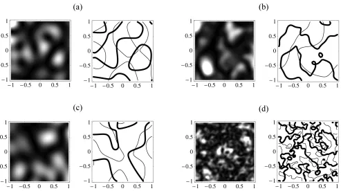
Figure 1: Simulated random superpositions of 200 waves, for each spectrum: (a) ring; (b) speckle; (c) shell; (d) Planck. Each plot is in units of the appropriate wavelength, and in each case, the left hand picture is of intensity ρ2 (with greater intensity being lighter), and the right hand plot is the contours ξ=0 (thick lines) and η=0 (thin lines). Note the dislocations, being the crossings of the contour pictures, correspond to dark regions in the intensity plots.
Examples of the intensity patterns and real and imaginary contours of these different spectra are given in fig 1, and the field autocorrelation functions are given in fig 2.
[image:5.595.145.445.490.678.2]4.
STATISTICAL DISLOCATION DENSITY AND ELLIPSE ECCENTRICITY
The details of calculations in this and subsequent sections can be found in 10. The eccentricity ε of the anisotropy ellipse described in section 2 may be calculated, and is independent of the spectrum. The ellipse in the has a higher eccentricity than the ellipse transverse to a dislocation line in space (as expected when obliquely slicing an elliptic cylinder):
ε 3 3π ε 2
8 2 0 8330
3
2 0 8697
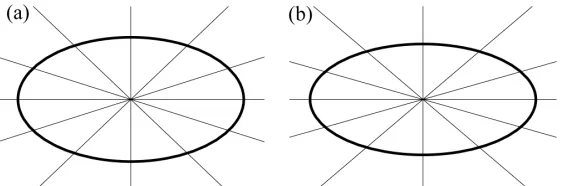
,d = = . , ,d = arcsinh1 - 1= . . (28) These ellipses, along with their phase spokes pattern, are given in fig 3.
Figure 3: Ellipses with the mean eccentricities given in (28): (a) transverse to a dislocation line in space; (b) in the plane. Equiphase lines are plotted at intervals of π/6, demonstrating the angular momentum phase relation described in section 2.
The dislocation line densityd3, the average length of dislocation line per unit volume, is given by
d3 k2 k2
3 0 1061
= δ ξ δ η = δ ξ δ η ξ∇ × ∇η = = π
( ) ( )ωω ( ) ( ) . , (29)
and the corresponding planar dislocation point density d2 (average number of dislocation points in the plane) is
d2 z x y y x K2 k2
4 6
= δ ξ δ η ω = δ ξ δ η ξ η −ξ η = =
π π
( ) ( ) ( ) ( ) , (30)
where the last equality only applies for plane sections of waves in space. A measure of the mean spacing of dislocation points in the plane is given by 1/√d2. It is, in fact, easy to show that d2/d3=1/2 is general, since d2 involves the flux of |ωω|ωω through the x,y plane, that is, its z component; the average length of the z component of a random unit vector can easily be shown to be 1/2, whereas the length of a unit vector is always 1.
The value calculated for d3 may also be compared to the corresponding density of singularities for isotropic complex gaussian random vector waves in three dimensions (that is, lines where the polarisation ellipse is circular (C lines) and linear (L lines))25, 26:
d3 3 k2 k2 d3 k2
10 1
5 3 0 2110 0 2136
,C= π + = . , ,L = . . (31)
These values are very close numerically, but are not equal. Also, they are both very close to 2d3 (29), that is, twice the corresponding dislocation density. It is not immediately obvious why these relations should exist (although it is likely that the C line result is related to the fact that C lines can be taken as dislocations in the scalar field received by taking the inner product of the complex vector field with itself 26). The two dimensional results for the four particular spectra are presented in table 1.
Spectrum Ring Shell Speckle Planck
d2 π/Λ02 2π/3λ02 2π/Λσ2 80 π3/63λT2
Mean spacing (1/√d2) 0.564 Λ0 0.691 λ0 0.399 Λσ 0.156 λT
1/√d2,C − 0.490 λ0 − 0.113 λT
[image:6.595.159.441.193.286.2]1/√d2,L − 0.487 λ0 − 0.112 λT
5.
DISLOCATION CORRELATIONS
The positions of dislocations in the plane are not independent, but are correlated, the precise nature of which depending on the field autocorrelation C(R) defined in (18). The correlations calculated are of two types: the number correlation function g(R), which averages local dislocation number densities separated by a distance R, and the charge correlation function gQ(R), which averages local charge densities separated by R. Using the same suffixes A,B as in (18), g(R) is given by
g R d
C C C
C C Y Z ZU U ZF ZE
YU Z X Y F
A A z A B B z B
p p p m ( ) ( ) ( ) ( ) ( ) ( ) ( ) ( ) ( ) , , = =
(
′ + ′′ −)
′′ − − + −[
− − + + − + + + 1 2 11 2 2 2 2 4 4
2 2 1
22 2
0 2
0 2 2
δ ξ δ η ω δ ξ δ η ω
π
i
Π
(
UEUEm+ Y m)
]
2 Π ,
(32)
where C0′′ ≡ ′′C ( )0 =d2 2π, and
F F V U V
F F V V U
p m =
(
[
]
)
=(
−[
]
)
i arcsinh i arcsinh / , / , 2 2E E V U V
E E V V U
p m =
(
[
]
)
=(
−[
]
)
i arcsinh i arcsinh / , / , 2 2 (33) Π Π Π Π p mV V U V
V V V U
=
(
[
]
)
=(
−[
]
)
2 2 2 2 ; / , ; / , i arcsinh i arcsinhwhere F,E,Π in (33) are the (incomplete) elliptic functions of the first, second and third kinds respectively (with the conventions for elliptic functions being those used by Mathematica27). Also,
U X Y Z
V X Y Z
= + − + = − − +
1
1
,
, (34)
and finally,
X
C C C C RC RCC C C C C C RC RCC C
R C C C C
Y C CC C C
R
=
(
′ + ′′ − ′ + ′′ + ′ ′′)
(
′ + ′′ − ′ − ′′ − ′ ′′)
′′(
′′ − + ′)
= ′
(
′ + ′′ −)
3
0 2 2 0 3 0 2 2 0
2
02 0 2 2 2
2 2 2 2
2 1 1 1 1 ( )( ) ( )( ) ( ) , ( ) ′′′
(
′′ − + ′)
= − ′′ − ′(
′ + − ′′ + ′′)
(
′ + + ′′ − ′′)
′′(
′′ − + ′)
C C C C
Z
C R C C C C C C C C C C
R C C C C
02 0 2 2 2
2 2
02 2 2 0 2 0
2
02 0 2 2 2
1
1 1 1
1 ( ) , ( )( ) ( )( ) ( )( ) ( ) . (35)
gQ(R) is defined in the same way as g(R), but weighted by dislocation strength (5),
g R d
C CC C C
R C C C R
C C
Q A A z A B B z B
R ( ) ( ) ( ) ( ) ( ) ( ) ( ) , , , = = ′
(
′ + ′′ −)
′′ −(
)
= ′′ ′ − 1 2 1 1 1 1 22 2 2 0 2 2 02 2 2δ ξ δ η ω δ ξ δ η ω
∂
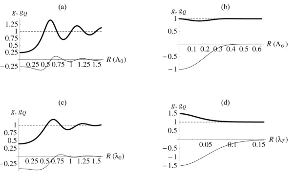
Figure 4: The number correlation function g(R) (thick line) (with asymptotic value 1 (dashed line)), as given in (32), and charge correlation function gQ(R) (thin line), as given in (36), for the four spectra: (a) ring; (b) speckle; (c) shell; (d) Planck;
in appropriate units of wavelength.
with the first term on the second line of (36) being a special case of a general expression obtained by Halperin28. g,gQ for the four spectra can be seen in fig 4. It can be shown that
g( )0 = −gQ( )0, (37)
a property shared by the first and second derivatives as well, as is apparent from the fig 4. Note that, for a random distribution of signed points in the plane (Poisson distribution), g=1 gQ=0 always, and there is no correlation between
points. These values are approached asymptotically for each of the spectra, as the degree of correlation reduces with distance.
There is a good analogy between the two statistical theories of signed dislocations in the plane and ionic liquids29 (such as molten salts), for which many mathematical techniques have been developed. However, caution must be taken not to take this analogy too far; the two theories are completely different physically, and some similarities may be coincidental. For example, the ring and shell correlation functions (fig 4a,c) have oscillations, a feature common to ionic liquids (see eg 29 p34), but have different physical explanations: In the ionic case, the oscillations are due to packing restrictions due to the finite size of the ions, but for dislocations, which can be arbitrarily close, they arise from the sharpness in the spectrum Π (for the smooth speckle and Planck spectra, there are no oscillations). It is interesting that the tools developed for such ionic theories are powerful enough to handle the completely different physics of dislocations in complex wavefields; use of these theories has been made by Hannay30 in a different context again. A useful concept from the ionic theory is the notion of partial correlation functions between the different species, defined as
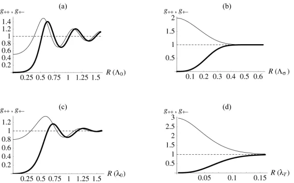
g++ =g−− ≡ +g gQ, g+− ≡ −g gQ, (38)
which are shown for the four spectra in fig 5. By (37) and the discussion following, g++(0)=0, a zero which is at least cubic, so like charges are statistically repulsive; they cannot dynamically repel, at least for monochromatic waves, because the dislocation patterns are stationary - rather it is unlikely to find two like charges close to each other, justifying the claim that only strength ±1 dislocations are generic. There is no such restriction on unlike charges, and there are no such properties for the Poisson distribution, whose points are completely independent, and in this case g++= g+-=1 always.
Figure 5: The partial correlation functions g++, (thick line), g+- (thin line) defined by (38), with their asymptotic value 1 (dashed line), for the four spectra: (a) ring; (b) speckle; (c) shell; (d) Planck; in appropriate units of wavelength.
of local neutrality, expressed by the screening relation
2 2 1
0
πd dRRgQ( )R = −
∞
∫
, (39)that is, the integral of the charge throughout the rest of the plane must compensate the strength of a dislocation centred to the origin. (39) is known in ionic liquid theory as the first Stillinger-Lovett sum rule33, 34. The second Stillinger-Lovett sum rule maintains that the second moment of R with respect to gQ is of the order of the screening length, that is, the effective
distance over which the charge is screened by (39). However, for the ring and shell spectra, the second moment of gQ
diverges, implying an effectively infinite length over which each charge is screened. This long-range correlation property leads to other interesting features for wavefields with these spectra, which are currently being investigated. For the speckle and Planck spectra, the screening lengths are comparable with to ranges of the functions as seen in figs 4,5,b,d. For the Poisson distributions of signed points, of course, there is no screening.
The screening property can be understood more clearly when one considers the total charge Q(N) of dislocations in a large area A=N/d2 (ie N>>1). Clearly, the average charge 〈Q(N)〉=0, but screening affects the mean square fluctuation
〈Q(N)2〉. If the charges merely have average (global) neutrality, there are no long-range correlations, and 〈Q(N)2〉~N. This is the case for random Poisson dots, and also for dislocations when edge effects are not neglected35, which is done here by Gauss-smoothing the (circular) area A. In this case, for any N, it can be shown that
Q N N d RRg R R
A
RR C C
R A
Q 2
2
2
0
0
2
2
2 1
2 1 2 2
1
4 1 2
( ) ( ) exp
exp ,
= + −
= ′
−
−
∞
∞
∫
∫
π π
π
d
d
(40)
where the second equality is derived using (36),(39). The first equality shows that, without screening, the leading term for large N would be N/2, and the fluctuations would be those of the Poisson distribution, with merely average neutrality. However, for dislocations there is screening, and
Q N RR C
C O N
2 2
2 0
1 1
4 1
( ) = ′ ( )
−
+ ∞
−
∫
d , (41)The other correlation functions, g, g++, g+- can be used for a crude Poisson approximation of the nearest neighbour probability density functions P(R), P++(R), P+-(R), that is the probability that the nearest appropriately signed neighbour is at distance R from a dislocation. The probability that the nearest neighbour is at a distance R from the dislocation is estimated to be the probability of there being no dislocations in small annular rings R1,R2,…,RM-1, separated by small distances dRi,
and R=RM, the approximation being that the dislocations in each annulus are independent; a proper calculation would
involve all multipoint correlation functions between these dislocations. Under this approximation,
P R R d g R R R d g R R Ri i i
i M
( )d = ( ) d
(
− ( ) d)
= −
∏
2 2 1 2 2
1 1
π π , (42)
and, in the limit M→∞, dR→0,
P R d Rg R d SSg S
R
( )= ( ) exp− ( )
∫
2 2 2 2
0
π π d , (43)
[image:10.595.146.445.359.550.2]and P++,P+-,g++,g+- replace P,g where appropriate. The probability densities for the four spectra are shown in fig 6; note that for Poisson points, all three distributions are identical Poisson probability distributions (in fact, this is where the name for such a distribution comes from). For dislocations, it is evident that the nearest oppositely charged neighbour is statistically closer than the nearest identically charged neighbour, as one expects from the statistical repulsion of like charges. The measure of mean spacing, used for example in table 1, possibly overestimates this spacing, but is consistent for each spectrum. Berggren and coworkers12 have refined the ring spectrum calculation of nearest neighbour spacings with the Bernoulli approximation (which includes some degree of multipoint correlation), and have found good agreement between the theory and numerical experiment.
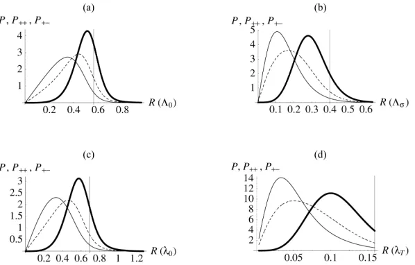
Figure 6: The (approximate) nearest neighbour probability density functions P (dashed line), P++ (thick line), P+- (thin line) derived in (43), for the four spectra: (a) ring; (b) speckle; (c) shell; (d) Planck. The vertical line gives the approximate mean spacing from 1/√d2, as given in table 1.
6.
ACKNOWLEDGEMENTS
7.
REFERENCES
1. S. O. Rice, “Mathematical analysis of random noise,” Bell. Syst. Tech. J.24, pp. 46-156, 1945. 2. S. O. Rice, “Mathematical analysis of random noise,” Bell. Syst. Tech. J.23, pp. 282-332, 1944. 3. N. Wax, Selected Papers on Noise and Stochastic Processes, New York:Dover, 1954.
4. R. C. Bourret, “Coherence properties of blackbody radiation,” Nuovo Cim.18, pp. 347-356, 1960.
5. L. Mandel and E. Wolf, Selected Papers on Coherence and Fluctuations of Light, vol. I, New York:Dover, 1970. 6. M. S. Longuet-Higgins, “Reflection and refraction at a random moving surface. II. Number of specular points in a
Gaussian surface,” J.Opt.Soc.Amer.50, pp. 845-850, 1960.
7. M. S. Longuet-Higgins, “Reflection and refraction at a random moving surface. III. Frequency of twinkling in a Gaussian surface,” J.Opt.Soc.Amer.50, pp. 851-856, 1960.
8. J. W. Goodman, Statistical Optics, New York:Wiley, 1985.
9. W. Feller, An Introduction to Probability Theory and Its Applications, vol. I, 3rd edn. New York:Wiley, 1950. 10. M. V. Berry and M. R. Dennis, “Phase singularities in isotropic random waves,” Proc. Roy. Soc. Lond. A456, pp.
2059-2079, 2000.
11. M. V. Berry and M. R. Dennis, “Phase singularities in isotropic random waves (corrigenda),” Proc. Roy. Soc. Lond. A456, pp. 3050, 2000.
12. A. I. Saichev, K.-F. Berggren and A. F. Sadreev, “Distribution of nearest distances between nodal points for the Berry function in two dimensions,” Phys. Rev. E (submitted), 2000.
13. L. Rayleigh, “On the character of the complete radiation at a given temperature,” Phil. Mag.27, pp. 460-469, 1889. 14. A. Einstein and L. Hopf, “On a theorem of the probability calculus and its application to the theory of radiation,”
Ann. Phys.33, pp. 1096-1104, 1910.
15. A. Einstein and L. Hopf, “Statistical investigation of a resonator's motion in a radiation field,” Ann. Phys.33, pp. 1105-1115, 1910.
16. L. Mandel and E. Wolf, Optical Coherence and Quantum Optics, Cambridge:University Press, 1995. 17. J. F. Nye and M. V. Berry, “Dislocations in wave trains,” Proc. Roy. Soc. Lond.A336, pp. 165-90, 1974. 18. J. F. Nye, Natural focusing and fine structure of light, Bristol:Institute of Physics Publishing, 1999. 19. M. S. Soskin, Proc. Int. Conf. onSingular Optics, SPIE vol. 3487, Bellingham, Washington:SPIE, 1998. 20. M. Vasnetsov and K. Staliunas, Optical vortices, Commack, New York:Nova Science Publications, 1999. 21. V. I. Arnold, Mathematical Methods of Classical Mechanics, 2nd edn. New York:Springer, 1989.
22. L. Allen, M. J. Padgett and M. Babiker, “The orbital angular momentum of light,” in Progress in Optics, vol. 39, pp. 291-372, 1999.
23. M. V. Berry, “Regular and irregular semiclassical wave functions,” J. Phys. A10, pp. 2083-91, 1977.
24. K.-F. Berggren, K. N. Pichigin, A. F. Sadreev and A. Starikov, “Signatures of quantum chaos in the nodal points and streamlines in electron transport through billiards,” JETP Lett.70, pp. 403-409, 1999.
25. J. F. Nye and J. V. Hajnal, “The wave structure of monochromatic electromagnetic radiation,” Proc. Roy. Soc. Lond.A409, pp. 21-36, 1987.
26. M. V. Berry and M. R. Dennis, “Polarization singularities in isotropic random vector waves,” Proc. Roy. Soc. Lond.A457, pp. 141-155, 2001.
27. S. Wolfram, The Mathematica Book, 3rd edn. Cambridge:University Press, 1996.
28. B. I. Halperin, “Statistical mechanics of topological defects,” in Les Houches Lecture Series, vol. 35, R. Balian, M. Kléman and J.-P. Poirier, Eds. Amsterdam: North-Holland, pp. 813-857, 1981.
29. J.-P. Hansen and I. R. McDonald, Theory of simple liquids, New York:Academic Press, 1986.
30. J. H. Hannay, “Chaotic analytic zero points: exact statistics for those of a random spin state,” J. Phys. A.29, pp. L101-L105, 1996.
31. I. Freund and N. Shvartsman, “Wave-field phase singularities: The sign principle,” Phys. Rev. A.50, pp. 5164-5172, 1994.
32. N. Shvartsman and I. Freund, “Wavefield phase singularities: near-neighbour correlations and anticorrelations,” J. Opt. Soc. Amer. A.11, pp. 2710-2718, 1994.
33. F. H. Stillinger and R. Lovett, “Ion-pair theory of concentrated electrolytes. I. Basic concepts,” J. Chem. Phys.48, pp. 3858-3868, 1968.
34. F. H. Stillinger and R. Lovett, “General restriction on the distribution of ions in electrolytes,” J. Chem. Phys.49, pp. 1991-1994, 1968.