L
1
-induced Performance Analysis and Sparse
Controller Synthesis for Interval Positive Systems
Xiaoming Chen, James Lam, Ping Li, and Zhan Shu
Abstract—This paper is concerned with the design of L1
-induced sparse controller for continuous-time positive systems with interval uncertainties. A necessary and sufficient condition for stability and L1-induced performance of positive linear
systems is proposed in terms of linear inequalities. Based on this, conditions for the existence of robust state-feedback controllers are established. Moreover, the total number of all the nonzero elements of the controller gain is to be minimized, while satisfying a guaranteed level ofL1-induced performance. Then,
we propose anℓ1-minimization problem to relax theℓ0objective
function for optimization and an iterative convex optimization approach is developed to solve the conditions. Finally, an illustrative example is provided to show the effectiveness and applicability of the theoretical results.
Index Terms—Interval uncertainties, Linear Lyapunov func-tions,L1-induced performance, Positive systems, Sparse control.
I. INTRODUCTION
I
N many practical systems, there is such a kind of systems whose state variables are confined to be positive. Such systems are frequently encountered in various fields, for in-stance, ecology [1], industrial engineering [2]. These systems belong to the class of positive systems, whose state variables and outputs take only nonnegative values for nonnegative inputs and initial conditions. Positive systems possess many special characteristics, mainly due to the fact that the states of positive systems are confined within a cone located in the positive orthant rather than in the whole space. The special characteristics brings about many new issues, which cannot be solved in general by using well-established methods for general linear systems. Therefore, the study on positive system theory has drawn the attention of many researchers all over the world in recent years.After a system-theoretic approach to positive systems was proposed in [3], a large number of theoretical contributions have appeared in the literature [4], [5], [6], [7], [8]. Among these research results, a positive state-space representation of a given transfer function has been characterized in [9]. Necessary and sufficient conditions for positive realizability by means of convex analysis have been derived in [10]. Reachability and controllability for positive systems have been investigated thoroughly in [11] and [12]. The syn-thesis problem of state-feedback controllers guaranteeing the closed-loop system to be positive and asymptotically stable has been investigated by the LMI approach and the linear programming approach in [13] and [14], respectively.
Manuscript received March 18, 2013; revised April 11, 2013. This work was partially supported by GRF HKU 7138/10E.
X. Chen, J. Lam and P. Li are with the Department of Mechanical Engineering, The University of Hong Kong, Pokfulam Road, Hong Kong (Emails: [email protected]; [email protected]; [email protected]).
Z. Shu is with the Electro-Mechanical Engineering Group, Faculty of Engineering and the Environment, University of Southampton, UK (Email: [email protected]).
Stability theory for nonnegative and compartmental dynamic systems with time delay has been investigated in [15], [16], [17]. Some results on 2-D positive systems can be found in [7], [18]. As for the results on model reduction problem for positive systems, we refer readers to [19], [20].
Although numerous results have been developed, it is noted that most of the above mentioned research works are based on quadratic Lyapunov functions. The results are often formulated under the linear matrix inequality (LMI) frame-work [21]. In recent years, some new results based on linear Lyapunov functions have emerged [14], [22], [23], [24]. The motivation is that the state of positive systems is nonnega-tive, making a linear Lyapunov function a valid candidate. However, the above-mentioned works mainly focused on the stability analysis problem and less efforts have been made in designing the controllers for positive systems. In addition, some frequently used costs such asH∞ norm are based on theL2signal space [25] and these costs are not very natural to describe some of the features of practical physical systems. By contrast, 1 norm provides a more useful description for positive systems, for instance, if the values represent the amount of material or the number of animal in a species. On the other hand, finding sparse vectors is important in many applications such as in parameter estimation or identification, signal processing or model reduction [26], [27]. A vector or signal is said to be sparse, if most of its entries are zero. The
ℓ0-norm quantifies sparsity by counting the number of non-zero entries in a vector or signal. However, finding sparse vectors is difficult because minimizing theℓ0-norm is a non-convex problem. In compressive sensing, sparse signals are reconstructed by replacing the ℓ0-minimization with an ℓ 1-minimization [27], [28]. However, there are few results on sparse controller synthesis for positive systems, especially with linear Lyapunov functions. Moreover, it is worth noting that the system parameters are usually assumed to be exactly known in the literature [29], [30]. Actually, practical systems are often affected by environmental changes, variations, per-turbations or disturbances, and consequently it is inevitable that uncertainties enter the system parameters [31]. Owing to the complexity caused by parameter uncertainties, the synthesis problems for uncertain positive systems have not been fully investigated. Motivated by the aforementioned discussions, in this paper, we consider the sparse state-feedback stabilization problem for continuous-time interval positive systems underL1-induced performance.
design problem is formulated by minimizing theℓ0-norm of the controller gain K and the ℓ0-optimization problem is relaxed by aℓ1-minimization problem. Moreover, the result-ing problem can be tackled by findresult-ing a solution of iterative convex optimization problems. An examples is provided in Section V to show the effectiveness and applicability of the theoretical results. Conclusions are given in Section VI.
II. PROBLEMFORMULATION
In this section, we introduce notations and several results concerning continuous-time linear positive systems.
LetRbe the set of real numbers;Rndenotes then-column real vectors;Rn×mis the set of all real matrices of dimension
n×m. LetR¯n
+ denote the nonnegative orthants ofRn; that is, if x ∈ Rn, then x ∈ R¯n
+ is equivalent to x ≥≥ 0. N is the set of natural numbers. For a matrix A ∈ Rm×n,
aij denotes the element located at the ith row and the jth column. A ≥≥ 0 (respectively, A >> 0) means that for all i and j, aij ≥ 0 (respectively, aij > 0). The notation
A ≥≥ B (respectively, A >> B) means that the matrix
A −B ≥≥ 0 (respectively, A −B >> 0). The matrix
A∈Rn×n is called Metzler, if all its off-diagonal elements are positive, that is, ∀(i, j), i ̸= j, aij ≥ 0. For matrices
A, A, A ∈ Rn×m, the notation A ∈ [A, A] means that
A≤≤A≤≤A. The symbolcoli(A)denotes theithcolumn of matrix A. The superscript “T” denotes matrix transpose.
∥·∥ represents the Euclidean norm for vectors. The 1-norm of a vector x(t) = (x1(t), x2(t), . . . , xn(t)) is defined as
∥x(t)∥1 , n
∑
i=1
|xi(t)| and the induced 1-norm of a matrix
Q,[qij]∈Rm×n is denoted by ∥Q∥1 , max 1≤j≤n(
m
∑
i=1
|qij|). The L1-norm of x is defined as ∥x∥L1 ,
∫∞
0 ∥x(t)∥1dt. The all-ones vector in Rn is denoted by 1n. Given a matrix
A= [a1, . . . , an]with ai being its ith column, we define a vector vec(A),[aT
1 . . . aTn]T. Matrices, if their dimensions are not explicitly stated, are assumed to have compatible dimensions for algebraic operations.
Consider an interval system:
{
˙
x(t) = Ax(t) +Bww(t),
y(t) = Cx(t) +Dww(t),
(1)
wherex(t)∈Rn, w(t)∈Rm andy(t)∈Rr are the system state, input and output, respectively.
In this paper, the system matrices A,Bw,C andDw are not precisely known, but belong to the following admissible uncertainty domain:
A∈[A, A], Bw∈[Bw, Bw], C∈[C, C], Dw∈[Dw, Dw]. (2) We have the following definitions throughout the paper. Definition 1: For a vector x = [x1, . . . , xn]T ∈ Rn, it is called sparse if its ℓ0-norm is small compared to the dimension of the vector, whereℓ0-norm ofxis defined as
∥x∥0= n
∑
i=1
|sign(xi)|.
Definition 2: System (1) is said to be a continuous-time positive linear system if for allx(0)≥≥0 andw(t)≥≥0, we have x(t)≥≥0 andy(t)≥≥0 fort >0.
Definition 3: System (1) is said to be positive and robustly stable if it is positive and asymptotically stable over all admissible uncertainty domain in (2).
In the following, we introduce some useful results which will be used in the sequel.
Lemma 1 ([32]): The system in (1) is a continuous-time positive linear system if and only if
A is Metzler, Bw≥≥0, C≥≥0, Dw≥≥0.
Proposition 1 ([22]): The positive linear system given by (1) is asymptotically stable if and only if there exists a vector
p≥≥0 (orp >>0) satisfying
pTA <<0. (3)
Lemma 2 ([27]): The convex envelope of the function
f =∥x∥0=
n
∑
i=1
|sign(xi)| onX ={x∈Rn|∥x∥∞≤1} is
fenv(x) =∥x∥1= n
∑
i=1
|xi(t)|.
Now, we are in a position to give the definition of L1 -induced norm. For a stable positive linear system given in (1), itsL1-induced norm is defined as
∥ℑ∥(L1,L1), sup
w̸=0, w∈L1
∥y∥L1
∥w∥L1
, (4)
whereℑ :L1 →L1 denotes the convolution operator, that is,y(t) = (ℑ∗w)(t). We say that system (1) hasL1-induced performance at the levelγif, under zero initial conditions,
∥ℑ∥(L1,L1)< γ, (5)
whereγ >0 is a given scalar.
III. PERFORMANCEANALYSIS
In this section, we compute the exact value ofL1-induced norm for positive system (1). Then, the performance charac-terization is provided for positive system (1) over the whole uncertain domain in (2).
First, we give the following theorem through which the value of L1-induced norm of system (1) can be computed directly.
Theorem 1: For a stable positive linear system given in (1), the exact value of theL1-induced norm is given by
∥ℑ∥(L1,L1)=∥Dw−CA
−1B
w∥1. (6) Proof: For system (1), the impulse response G(t) is given by
G(t),
{
0, t <0,
CeAtBw+Dwδ(t), t≥0.
(7)
Next, letℑ:L1→L1 denote the convolution operator:
z(t) = (ℑ ∗w)(t),
∫ ∞
0
G(t−τ)w(τ)dτ. (8)
From [33], we have
∥ℑ∥(L1,L1)=j=1max,...,m∥colj( ¯G)∥1, (9)
where
¯
Gij =
∫ ∞
0
Letci,bwj,dwij denote theithrow vector, the jthcolumn vector and the (i, j)-element of matrices C, Bw and Dw, respectively. Equation (10) can be written as
¯
Gij =
∫ ∞
0
(
cieAtbwj+dwijδ(t)
)
dt=−ciA−1bwj+dwij, (11)
yielding (6).
Next, we derive the following result which provides a fundamental characterization on the stability of system (1) with the performance in (5).
Theorem 2: The positive linear system in (1) is asymp-totically stable and satisfies ∥y∥L1< γ∥w∥L1 if and only if
there exists a vector p≥≥0satisfying
1TrC+pTA << 0, (12)
pTBw+1TrDw−γ1Tm << 0. (13)
Proof:(Sufficiency) In the following, we consider two cases:
x(t) ≡ 0 and there exists a t such that x(t) ̸= 0. First, for x(t) ≡0, from (12), the asymptotic stability of system (1) is proved. It is easy to see that if x(t) ≡ 0, we have
y(t) =Dww(t)and from (13),∥y∥L1 < γ∥w∥L1 holds.
Next, we assume that there exists at such that x(t)̸= 0. From (12), we can see that (3) holds, and thus the asymptotic stability of system (1) is proved.
Consider the linear Lyapunov function candidate
V(x(t)) =pTx(t)and we have
dV(x(t))
dt =p
T(Ax(t) +B ww(t)). Let
J=
∫ T
0
∥y(t)∥1dt−
∫ T
0
γ∥w(t)∥1dt
=
∫ T
0
( r
∑
i=1
yi(t)−γ m
∑
i=1
wi(t)
) dt
=
∫ T
0
( r
∑
i=1
yi(t)−γ m
∑
i=1
wi(t) +
dV(t)
dt )
dt−V(T)
=
∫ T
0
([
1TrC+pTA]x(t) + (1TrDw+pTBw
−γ1Tm)w(t))dt−V(T) =
∫ T
0
([
1TrC+pTA+ε1Tn]x(t) + (1TrDw
+pTBw−γ1Tm)w(t)
)
dt−
∫ T
0
ε1Tnx(t)dt−V(T),
where ε >0 is sufficiently small such that 1T
rC+pTA+
ε1T
n <<0holds.
From (12) and (13), we have
J+
∫ T
0
ε1Tnx(t)dt+V(T)<0, which equals to
∫ T
0
( r
∑
i=1
yi(t)
)
dt+ε
∫ T
0
( n
∑
i=1
xi(t)
) dt
< γ
∫ T
0
(m
∑
i=1
wi(t)
)
dt−pTx(T).
Since the system is asymptotically stable, whenT → ∞we have
∫ ∞
0
( r
∑
i=1
yi(t)
)
dt+ε
∫ ∞
0
( n
∑
i=1
xi(t)
) dt
≤γ
∫ ∞
0
(m
∑
i=1
wi(t)
) dt,
which implies
∥y∥L1 < γ∥w∥L1. (14)
This proves sufficiency.
(Necessity) Assume that system (1) is asymptotically sta-ble and satisfies ∥y∥L1 < γ∥w∥L1. Then, according to
Theorem 1, the following inequality holds
∥Dw−CA−1Bw∥1< γ, (15)
which implies
1TrDw−1TrCA− 1B
w−γ1Tm<<0. (16)
Definep˜,(−1T
rCA−1)T ≥≥ 0 andp,p˜+ϵξ >>0, where ξ >> 0 satisfies ξT(−A) >> 0, and ϵ > 0 is a sufficiently small number. We have
1TrC+pTA = 1TrC+ (˜pT+ϵξT)A
= 1TrC−1TrC+ϵξTA
= ϵξTA
<< 0. (17)
On the other hand,
1TrDw+pTBw−γ1Tm
=1TrDw−1TrCA− 1B
w+ϵξTBw−γ1Tm.
From (16) andϵ >0is sufficiently small, we have that (13) holds. This completes the whole proof.
Remark 1: Theorem 2 presents a necessary and sufficient condition on theL1-induced performance of a stable positive system in terms of linear programming. A similar result, proven by virtue of dissipativity theory, can be found in [24]. In the following, we provide a theorem as the performance characterization for positive system (1) over the whole un-certain domain in (2).
Theorem 3: The positive linear system in (1) is robustly stable and satisfies ∥y∥L1 < γ∥w∥L1 for any A ∈ [A, A], C ∈ [C, C], Bw ∈ [Bw, Bw] and Dw ∈ [Dw, Dw] if and only if there exists a vectorp≥≥0 satisfying
1TrC+pTA << 0, (18)
pTBw+1TrDw−γ1Tm << 0. (19)
Proof:(Sufficiency) For anyA∈[A, A],C∈[C, C],Bw∈
[Bw, Bw]andDw∈[Dw, Dw],
1TrC+pTA≤≤1TrC+pTA, pTBw+1TrDw−γ1Tm≤≤p
TB
w+1TrDw−γ1Tm, which, by Theorem 2, implies that system (1) is robust stable and satisfies ∥y∥L1 < γ∥w∥L1 over all admissible
uncertainty domain. This proves sufficiency.
(Necessity) Assume that system (1) is robustly stable and satisfies ∥y∥L1 < γ∥w∥L1. From Theorem 2, we have (12)
and (13) hold, which implies that (18) and (19) hold. This
IV. SPARSESTATE-FEEDBACKCONTROLLERDESIGN
This section deals with the robust sparse state-feedback stabilization problem for positive systems with interval un-certainties.
The problem of L1-induced sparse controller design (L1SCD) is formulated as follows.
Problem L1SCD: Given a positive system
S:
{
˙
x(t) = Ax(t) +Bu(t) +Bww(t),
y(t) = Cx(t) +Du(t) +Dww(t),
(20)
whereA∈[A, A],B∈[B, B],Bw∈[Bw, Bw],C∈[C, C],
D ∈ [D, D] and Dw ∈ [Dw, Dw], find a state-feedback controller u(t) =Kx(t)such that
1) the closed-loop system
{
˙
x(t) = (A+BK)x(t) +Bww(t),
y(t) = (C+DK)x(t) +Dww(t),
(21)
is positive and robustly stable.
2) the ℓ0-norm of the controller gain K is minimized subject to theL1-induced performance, that is,
min∥K∥0
subject to∥y∥L1< γ∥w∥L1. (22)
This is a common sense approach which simply seeks the sparsest controller gainKsatisfying the constraint. However, the optimization problem is non-convex and NP-hard. From Lemma 2, we know that the ℓ0-optimization problem (22) can be relaxed by the followingℓ1-minimization problem:
min∥vec(K)∥1
subject to∥y∥L1 < γ∥w∥L1. (23)
Before solving the ℓ1-minimization problem (23), a nec-essary and sufficient condition is first presented for the existence of a solution to the L1-induced state-feedback stabilization problem. We supposeK≤≤0and the detailed proof is omitted here.
Theorem 4: Suppose K ≤≤ 0. The closed-loop system (21) is positive, robustly stable and satisfies ∥z∥L1 < γ∥w∥L1 for any A∈[A, A], B ∈[B, B], Bw ∈[Bw, Bw],
C∈[C, C],D∈[D, D]andDw∈[Dw, Dw]if and only if there exist a matrix K and a vectorp≥≥0satisfying
A+BK is Metzler, (24)
C+DK ≥≥0, (25)
1Tr(C+DK) +pT(A+BK)<<0, (26)
pTBw+1TrDw−γ1Tm<<0. (27)
Note that the Lyapunov vector p is coupled with the controller matrixK in (26), which cannot be easily solved. However, when matrix K is fixed, (26) turns out to be linear with respect to the remaining variables. Therefore, a natural way is to fix K, and solve (24)–(27) by linear programming. Thus, the following iterative algorithm can be proposed to solve Problem L1SCD.
Algorithm:
• Step 1. Seti= 1. Select an initial matrixK1 such that the system
{
˙
x(t) = Ax(t) +Bu(t) +Bww(t),
y(t) = Cx(t) +Du(t) +Dww(t),
(28)
with
u(t) =K1x(t) (29)
is positive and robustly stable.
• Step 2. For fixed Ki, solve the following feasibility problem forpi.
FP: Findpi subject to the following constraints:
1Tr(C+DKi) +pTi(A+BKi) << 0,
pTi Bw+1TrDw−γ1Tm << 0.
pi ≥≥ 0.
DenoteKi∗, pias the solution to the feasibility problem. If(Ki∗−Ki∗−1)/Ki∗< ε1, whereε1 is a prescribed bound, thenK∗=Ki,p=pi. STOP.
• Step 3. For fixed pi, solve the following optimization problem forKi.
OP: Minimize∥vec(K)∥1 subject to the following con-straints:
A+BKi is Metzler,
C+DKi≥≥0,
1Tr(C+DKi) +pTi(A+BKi)<<0.
DenoteKi∗ as the solution to the optimization problem.
• Step 4. If (Ki∗−Ki∗−1)/Ki∗ < ε2, where ε2 is a prescribed tolerance, STOP; else seti=i+ 1andKi=
Ki−1, then go to Step 2.
Remark 2: The initial matrixK1can be viewed as a state-feedback controller matrix, and can be constructed by exist-ing convex optimization approaches. From [13], we know that system (28) with (29) is positive and robustly stable if and only if there exist matrices P , diag(p1, p2, . . . , pn) andQ,[qij]∈Rl×n such that
P AT+QTBT+AP +BQ < 0,
aijpj+ l
∑
z=1
bizqzj ≥ 0, (1≤i̸=j≤n)
cijpj+ l
∑
z=1
dizqzj ≥ 0.
Under this condition, an initial choice ofK can be given by
K1=QP−1.
V. ILLUSTRATIVEEXAMPLE
In this section, we present an illustrative example to demonstrate the applicability of the proposed results.
Consider the following positive system:
{
˙
x(t) = Ax(t) +Bu(t) +Bww(t),
y(t) = Cx(t) +Du(t) +Dww(t),
(30)
0 2 4 6 8 10 0
2 4 6 8 10 12x 10
6
Time
Response
x1of System (A,B,Bw,Cz,Dz,C)
[image:5.595.87.248.57.189.2]x1of System (A,B,Bw,Cz,Dz,C)
Fig. 1: Time Response of Open-loop System
[C, C],D∈[D, D],Dw∈[Dw, Dw] with
A =
−02.50.00 −13.30.00 22..0000 2.00 1.50 −2.00
,
A =
−01.60.98 −12.31.96 22..0010 2.00 1.50 −1.92
,
B =
10..0000 01..0000 1.00 0.5
, B=
10..0404 01..0100 1.02 0.50
,
Bw =
00..4808 00..2000 0.00 0.50
, Bw=
00..5010 00..2100 0.02 0.52
,
C =
[
1.00 0.60 1.00 0.80 0.80 1.00
]
, D=
[
0.48 0.00 0.50 1.00
] ,
C =
[
1.02 0.61 1.00 0.80 0.82 1.00
]
, D=
[
0.50 0 0.52 1.01
] ,
Dw =
[
0.10 0.00 0.10 0.20
]
, Dw=
[
0.12 0.01 0.11 0.22
] .
Forγ = 0.7, by solving the conditions in Theorem 4 using Algorithm, we obtain the sparse controller gain
K∗ =
[
−0.6413 −0.5003 −1.7548
−0.0013 −0.0008 −0.0000
]
after 10iterations and a feasible solution is achieved with
p=[ 0.9761 0.7829 0.5888 ].
To illustrate the disturbance attenuation performance, the external disturbancew(t)is assumed to be
w(t) =
{ [
300 + 200 cos 2t e−3t ]T, t≤5,
[
0 0 ]T, otherwise,
and the initial condition used in the simulation is
x(0) =[ 500 200 300 ]T.
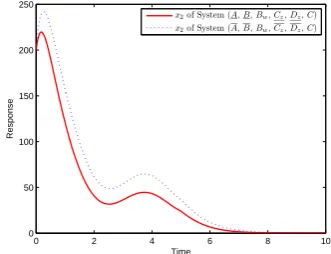
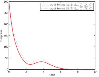
Figures 1–3 show the response of open-loop system and Figure 4–6 show the state response of the closed-loop system, from which we can see that the system can be stabilized by the designed controller.
0 2 4 6 8 10
0 1 2 3 4 5 6 7 8x 10
6
Time
Response
x2of System (A,B,Bw,Cz,Dz,C)
[image:5.595.343.506.228.360.2]x2of System (A,B,Bw,Cz,Dz,C)
Fig. 2: Time Response of Open-loop System
0 2 4 6 8 10
0 2 4 6 8 10 12x 10
6
Time
Response
x3of System (A,B,Bw,Cz,Dz,C)
[image:5.595.49.290.252.494.2]x3of System (A,B,Bw,Cz,Dz,C)
Fig. 3: Time Response of Open-loop System
0 2 4 6 8 10
0 50 100 150 200 250 300 350 400 450 500
Time
Response
x1of System (A,B,Bw,Cz,Dz,C)
x1of System (A,B,Bw,Cz,Dz,C)
Fig. 4: Time Response of Closed-loop System
0 2 4 6 8 10
0 50 100 150 200 250
Time
Response
x2of System (A,B,Bw,Cz,Dz,C)
x2of System (A,B,Bw,Cz,Dz,C)
Fig. 5: Time Response of Closed-loop System
VI. CONCLUSION
[image:5.595.340.507.402.533.2] [image:5.595.339.505.574.701.2]continuous-0 2 4 6 8 10 0
50 100 150 200 250 300
Time
Response
x3of System (A,B,Bw,Cz,Dz,C)
[image:6.595.85.252.61.191.2]x3of System (A,B,Bw,Cz,Dz,C)
Fig. 6: Time Response of Closed-loop System
time interval positive systems have been studied. A method has been derived to compute the exact value of the L 1-induced norm for positive systems and a characterization has been proposed to ensure the asymptotic stability of the positive system with a prescribed L1-induced performance level. In addition, the sparse controller design problem has been formulated by minimizing theℓ0-norm of the controller gain K, which has been relaxed by an ℓ1-minimization problem. Moreover, the resulting problem has been solved by an iterative convex optimization algorithm. Finally, an illustrative example is provided to show the effectiveness and applicability of the theoretical results.
REFERENCES
[1] H. Caswell, Matrix Population Models: Construction, Analysis and Interpretation. Sunderland, MA: Sinauer Assoc., 2001.
[2] L. Caccetta, L. R. Foulds, and V. G. Rumchev, “A positive linear discrete-time model of capacity planning and its controllability prop-erties,”Math. Comput. Model., vol. 40, pp. 217–226, 2004. [3] D. G. Luenberger,Introduction to Dynamic Systems : Theory, Models,
and Applications. New York: Wiley, 1979.
[4] E. Fornasini and M. Valcher, “Linear copositive Lyapunov functions for continuous-time positive switched systems,”IEEE Trans. Automat. Control, vol. 55, pp. 1933–1937, 2010.
[5] M. Valcher, “Reachability properties of continuous-time positive sys-tems,”IEEE Trans. Automat. Control, vol. 54, pp. 1586–1590, 2009. [6] P. Li, J. Lam, and Z. Shu, “H∞ positive filtering for positive linear discrete-time systems: An augmentation approach,”IEEE Trans. Automat. Control, vol. 55, no. 10, pp. 2337–2342, 2010.
[7] T. Kaczorek,Positive 1D and 2D Systems. Berlin, Germany: Springer-Verlag, 2002.
[8] Z. Shu, J. Lam, H. Gao, B. Du, and L. Wu, “Positive observers and dynamic output-feedback controllers for interval positive linear systems,”IEEE Trans. Circuits and Systems (I), vol. 55(10), pp. 3209– 3222, 2008.
[9] L. Benvenuti and L. Farina, “A tutorial on the positive realization problem,” IEEE Trans. Automat. Control, vol. 49(5), pp. 651–664, 2004.
[10] L. Farina, “On the existence of a positive realization,” Systems & Control Letters, vol. 28, pp. 219–226, 1996.
[11] M. P. Fanti, B. Maione, and B. Turchiano, “Controllability of multi-input positive discrete-time systems,”Int. J. Control, vol. 51(6), pp. 1295–1308, 1990.
[12] M. E. Valcher, “Controllability and reachability criteria for discrete time positive systems,”Int. J. Control, vol. 65(3), pp. 511–536, 1996. [13] H. Gao, J. Lam, C. Wang, and S. Xu;, “Control for stability and pos-itivity: equivalent conditions and computation,”IEEE Trans. Circuits and Systems (II), vol. 52, pp. 540–544, 2005.
[14] M. Ait Rami and F. Tadeo, “Controller synthesis for positive linear systems with bounded controls,”IEEE Trans. Circuits and Systems (II), vol. 54(2), pp. 151–155, 2007.
[15] W. Haddad, V. Chellaboina, and T. Rajpurohit, “Dissipativity theory for nonnegative and compartmental dynamical systems with time delay,”IEEE Trans. Automat. Control, vol. 49(5), pp. 747–751, 2004.
[16] X. Liu, W. Yu, and L. Wang, “Stability analysis of positive systems with bounded time-varying delays,”IEEE Trans. Circuits and Systems (II), vol. 56, pp. 600–604, 2009.
[17] L. Wu, J. Lam, Z. Shu, and B. Du, “On stability and stabilizability of positive delay systems,”Asian Journal of Control, vol. 11, pp. 226– 234, 2009.
[18] J. E. Kurek, “Stability of positive 2-D system described by the Roesser model,”IEEE Trans. Circuits and Systems (I), vol. 49, pp. 531–533, 2002.
[19] J. Feng, J. Lam, Z. Shu, and Q. Wang, “Internal positivity preserved model reduction,”Int. J. Control, vol. 83(3), pp. 575–584, 2010. [20] P. Li, J. Lam, Z. Wang, and P. Date, “Positivity-preservingH∞model
reduction for positive systems,”Automatica, vol. 47, no. 7, pp. 1504– 1511, 2011.
[21] S. Boyd, L. El Ghaoui, E. Feron, and V. Balakrishnan,Linear Matrix Inequalities in Systems and Control Theory. Philadelphia, PA: SIAM, 1994.
[22] W. Haddad, V. Chellaboina, and Q. Hui, Nonnegative and Com-partmental Dynamical Systems. Princeton, New Jersey: Princeton University Press, 2010.
[23] Y. Ebihara, D. Peaucelle, and D. Arzelier, “Optimal L1-controller
synthesis for positive systems and its robustness properties,” in Pro-ceedings of the American Control Conference, 2012.
[24] C. Briat, “Robust stability and stabilization of uncertain linear positive systems via integral linear constraints:L1-gain andL∞-gain
charac-terization,”Int. J. Robust & Nonlinear Control, vol. Published online, Dol: 10.1002/rnc.2859, 2012.
[25] W. Lu and G. Balas, “A comparison between Hankel norms and induced system norms,” IEEE Trans. Automat. Control, vol. 43(11), pp. 1658–1662, 1998.
[26] D. Donoho, “Compressed sensing,”IEEE Transactions on Information Theory, vol. 52, pp. 1289–1306, 2006.
[27] M. Fazel, “Matrix rank minimization with applications,” Ph.D. dis-sertation, Department of Electrical Engineering, Stanford University, 2002.
[28] S. Schuler, P. Li, J. Lam, and F. Allgower, “Design of structured dynamic output-feedback controllers for interconnected systems,” In-ternational Journal of Control, vol. 84, pp. 2081–2091, 2011. [29] X. Liu and C. Dang, “Stability analysis of positive switched linear
systems with delays,” IEEE Trans. Automat. Control, vol. 56, pp. 1684–1690, 2011.
[30] X. Liu, W. Yu, and L. Wang, “Stability analysis for continuous-time positive systems with time-varying delays,” IEEE Trans. Automat. Control, vol. 55, pp. 1024–1028, 2010.
[31] M. Kieffer and E. Walter, “Guaranteed parameter estimation for cooperative models,”Lecture Notes in Control Inf. Sci., vol. 294, pp. 103–110, 2003.
[32] L. Farina and S. Rinaldi,Positive Linear Systems: Theory and Appli-cations. Wiley-Interscience, 2000.